Observation of sub-Fourier resonances in a quantum-chaotic system

Abstract

We experimentally show that the response of a quantum-chaotic system can display resonance lines sharper than the inverse of the excitation duration. This allows us to discriminate two neighboring frequencies with a resolution nearly 40 times better than the limit set by the Fourier inequality. Furthermore, numerical studies indicate that there is no limit, but the loss of signal, to this resolution, opening ways for the development of sub-Fourier quantum-chaotic signal processing.

Any time-dependent signal can be characterized by its frequency spectrum, obtained by a Fourier transform. The Fourier inequality implies that getting a narrow frequency spectrum requires that the corresponding temporal signal lasts a long time. This inequality links the width $\Delta f$ of the frequency spectrum and the temporal width $\Delta t$ of the signal note:Fourier : $\Delta f\Delta t\geq 1/2$. A rule that is usually deduced from the above one states that two frequencies cannot be distinguished before a time proportional to the inverse of their difference. Of course, if the signal/noise ratio is infinite, two unresolved frequencies can still be distinguished using a good fit. This is not the problem we are here interested in. We rather concentrate on the raw width of a resonance signal, before any fit is performed. Physically, the Fourier inequality sets a limit to the minimum width of a resonance line to the inverse of the time duration of the experiment, a rule that applies also to quantum systems. For instance, the width of Ramsey fringes ref:Ramsey is limited by the time interval between the crossing times corresponding to the two Ramsey zones, and the frequency width of an atomic or molecular resonance absorption line is generally given by the inverse of the lifetime of the excited state. However, these conclusions rely on the linear relation between the system’s response to the excitation, and this limit can in principle be overcome provided a suitable non-linearity is introduced. The simplest example is to use a multiphoton resonance. Indeed, the frequency width of a $n$-photon excitation line is divided by a factor up to $n$ compared to a single photon excitation, as recently observed with multiphoton Raman transitions on atomic rubidium ref:Multiphoton . In this case, the sub-Fourier character originates from the fact that it is $n^{th}$ harmonic of the external driving frequency that has to be compared to the atomic frequency, and not the driving frequency itself. As a consequence, such a device is not very flexible, as it allows sub-Fourier lines only at subharmonics of the intrinsic atomic frequency. In the present paper, we show that, for a quantum system displaying chaos (which implies the presence of an intrinsic nonlinearity), sub-Fourier resonances can be widely observed, without the need of a resonance with some internal frequency of the system. They rely on a different process: the high sensitivity of a quantum chaotic device to periodicity breaking.

The system we studied is an atomic version of the quasiperiodically driven quantum kicked rotor described in ref:Bicolor . The periodic quantum kicked rotor ref:aQKR is a paradigmatic model for studies of time-dependent quantum-chaotic systems. Its atomic version has been implemented in recent experiments by many groups ref:Bicolor ; ref:eQKR ; ref:Raizen98 , and consists in placing a laser-cooled atomic cloud in a periodically pulsed, far-detuned ($\Delta_{L}\approx$ 9.2 GHz $\approx 1.7\times 10^{3}\Gamma$ in the present case), standing laser wave (SW). The atoms and the electromagnetic field then interact via the so-called “dipole” force ref:Dipole , which is conservative; the high laser-atom detuning insuring that dissipative effects due to spontaneous emission are negligible. The corresponding hamiltonian for a single atom is then, in convenient dimensionless units ref:Raizen98 :

$$H_{1}=\frac{P^{2}}{2}+K\cos\theta\sum_{n=1}^{N_{1}}\delta_{\tau}(t-n)$$ (1)

where time is measured in units of the kick period $T_{1}=1/f_{1}$, $P$ is the reduced momentum in units of $M/(2k_{L}T_{1})$ ($k_{L}$ is the laser wavenumber and $M$ the mass of the atom), $\theta=2k_{L}z$ the reduced position of the atom along the SW axis, $K=\Omega^{2}T_{1}\tau\hbar k_{L}^{2}/(2M\Delta_{L})$ the normalized kick intensity ($\Omega$ is the resonant Rabi frequency of the SW beams), $N_{1}$ the number of kicks, and $\delta_{\tau}(t)$ a Dirac-like square function of width $\tau$ with $\tau\ll T_{1}$ [$\delta_{\tau}(t)=1/\tau$ for $|t|\leq\tau/2$ and $\delta_{\tau}(t)=0$ elsewhere]. In the limit $\tau\rightarrow 0$, the dynamics of the system is entirely determined by two parameters: the kick intensity (or stochasticity parameter) $K$ and the effective Planck constant $\hbar_{\mathrm{eff}}=4k_{L}^{2}T_{1}\hbar/M$. For $K\gg 1$, the classical dynamics associated with the hamiltonian Eq. (1) is a chaotic, although perfectly deterministic, ergodic diffusion in phase space, and the mean kinetic energy $\langle P^{2}\rangle/2$ roughly grows linearly with time. Its quantum dynamics is however completely different, and displays a phenomenon known as “dynamical localization” (DL), which is a signature of quantum chaos ref:DL . DL consists in the suppression of the classical momentum diffusion (or a freezing of the wave packet evolution) after some localization time $t_{L}$, due to quantum destructive interferences among the various chaotic classical trajectories. For $t>t_{L}$, the average momentum distribution of the atom presents a characteristic time-independent exponential shape $p(P,t>t_{L})\sim\exp(-|P|/L)$, with a localization length in the momentum space given by $L$. DL is intimately related to the periodic character of the kick sequence, and bears a close analogy with Anderson’s localization in disordered solids ref:AndersonLoc .

The sensitivity of DL to deviations from exact periodicity is at the heart of the present experiment. Consider the following hamiltonian, consisting in two series of pulses of frequencies $f_{1}$ and $f_{2}$, with a ratio $r=f_{2}/f_{1}\approx 1$, and relative phase $\varphi$:

$$H_{2}=H_{1}+K\cos\theta\sum_{n=1}^{N_{2}<rN_{1}}\delta_{\tau}\big{(}t-\frac{n+\varphi/2\pi}{r}\big{)}$$ (2)

with the same normalizations as in Eq. (1). If $r=1$ (or, more generally, equal to any rational number), the perturbation is periodic and $H_{2}$ leads to dynamical localization. If the value of $r$ is slightly shifted from 1 and turns irrational, the kick series loses its temporal periodicity, DL disappears and the quantum evolution is on the average a continuous chaotic diffusion leading to arbitrarily large momenta. The dependence of the DL on the rational or irrational character of $r$ was recently observed experimentally ref:Bicolor . A fundamental question is: how fast can the quantum system distinguish between a true simple rational value of $r$ and a neighboring irrational value? The present experiment gives an unexpected response to this question.

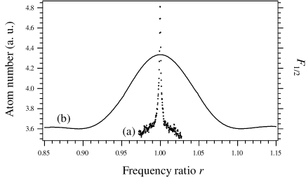
Figure 1: Below the Fourier limit. (a) Experimental measurement of the zero velocity atom number, $p(0)$, as a function of the ratio $r=f_{2}/f_{1}$ of the two excitation frequencies, for the following values of the parameters: $f_{1}=18$ kHz, $K=42$, $N_{1}=10$. The pulse duration is $\tau=3$ $\mu$s and in order to avoid pulses overlap we set $\varphi=\pi$. Averaging: 100 times. (b) $F_{1/2}(r)$, allowing comparison with the Fourier transform of the kick sequence, this curve is drawn with an arbitrary amplitude and offset.

In the experiment, a sample of cold cesium atoms issued from a standard magneto-optical trap is kicked by a far-detuned stationary wave (SW) with two series of kicks of frequencies $f_{1}$ and $f_{2}$ for a duration $T=N_{1}T_{1}$, according to the hamiltonian Eq. (2). The SW pulses are assumed to be short enough that the atomic motion during a pulse can be neglected, and the SW acts, with respect to atomic center of mass dynamics, as an instantaneous kick. Just after the end of the kick sequence, the number of zero momentum atoms $p(P=0)$ is probed with a Raman velocity selective excitation ref:Raman . Since the atom-number is conserved during the kick sequence, $p(0)$ is proportional to the inverse of the typical momentum at the end of the pulse sequence, i.e. $1/\sqrt{\langle P^{2}\rangle}$, and thus measures the degree of localization: the wider the momentum distribution, the smaller the value of $p(0)$. Whereas $f_{1}$ is kept constant, this procedure is repeated for various values of $f_{2}=rf_{1}$, leading to the resonance line shown in Fig. 1. As expected, this line has a maximum at $r=1$ where DL is present. A remarkable feature is that its width is extremely narrow and easily beats the standard Fourier limitation, with a $\Delta r_{\mathrm{exp}}=0.0026$, ($\Delta$ is the full width at half maximum, FWHM) and thus $\Delta f_{2}=f_{1}\Delta r_{\mathrm{exp}}\approx 47$ Hz, yielding:

$$\Delta f_{2}T\approx\frac{1}{38}\ll 1$$ (3)

Indeed, in a first approach, one would consider the frequency spectrum of the excitation formed by the two series of pulses. The Fourier spectrum of an infinite sequence of pulses of frequency $f_{1}$ is a comb of peaks separated by $f_{1}$. Since the sequence has a finite duration $T$, each peak in the Fourier transform has a width $1/T$. Furthermore, since the pulse duration $\tau$ is also finite, the whole spectrum is multiplied by the factor:

$$\left(\frac{\sin(\pi f_{1}\tau)}{\pi f_{1}\tau}\right)^{2}\text{ .}$$ (4)

When two sequences with slightly different frequencies are combined, the resulting Fourier spectrum has two series of peaks that may overlap. This is visible in Fig. 2, which shows, for different values of $r$, the squared modulus of the Fourier transform of the double kick sequence (with $\varphi=0$), in the neighborhood of the fundamental frequency $f_{1}$. Consider the function $F_{1/2}(r)$, defined as the squared modulus of the Fourier transform at frequency $f_{1/2}=(f_{1}+f_{2})/2=f_{1}(1+r)/2$. This function is large when the two peaks overlap and goes to zero when the two frequencies are completely resolved, giving a quantitative measure of the Fourier resolution. In order to make a comparison with the experimental data, $F_{1/2}(r)$ is also plotted in Fig. 1. Its width $\Delta F_{1/2}(r)$ is 0.091, and $\Delta F_{1/2}(r)/\Delta r_{\mathrm{exp}}\approx 35$, clearly showing that Fourier limit has been overcome.

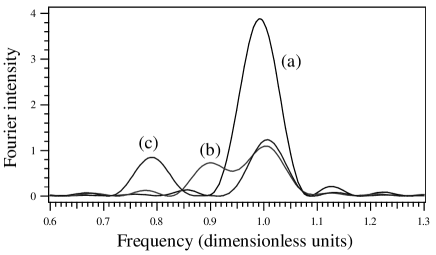
Figure 2: First harmonic of the Fourier transform of the kick sequence. The parameters are: $T=555$ $\mu$s, and $f_{1}=18$ kHz. (a) For $r=0.98$ the two frequencies are not resolved; (b) $r=0.93$ the two frequencies are barely resolved; (c) $r=0.80$, the two frequencies are clearly resolved. Note that the experimental resolution is $\Delta r_{\mathrm{exp}}=0.0026$, the frequency are thus well distinguished for $r\not\in[0.9987,1.0013]$.

If the width of the resonance line is not Fourier-limited, what is the origin of the process giving such a resolution? A first idea coming to mind is that each atom is not excited just by the fundamental frequencies $f_{1}$ and $f_{2}$, but also by their harmonics. The $j^{th}$ harmonic of each fundamental frequency has the same width $1/T$, but their frequency separation $j(f_{1}-f_{2})$ is increased by a factor $j$. One would thus attribute the high resolution of the system to the presence of the high harmonics in the excitation spectrum itself. In fact, this interpretation is invalid for several reasons. Firstly, the experimental kicks are not real $\delta$-peaks, but have a finite duration $\tau$ which implies that the weights of the high harmonics are small. For instance, with $\tau=3$ $\mu$s, as for the curve shown in Fig. 1, only harmonics up to $j=18$ lie in the central lobe of function (4). The harmonic $j=35$, whose frequency separation would corresponds to the experimental resolution observed in Fig. 1, lies beyond the first lobe with a very small intensity (less than 2% of the intensity of the first harmonic). Secondly, when $\tau$ is increased, with a constant pulse height (which implies that $K$ is increased, as it is proportional to $\tau$), the relative weight of the high harmonics decreases, because of the factor Eq. (4). But we verified both experimentally and numerically that the system’s resolution increases: the resonance lines becomes narrower (see Fig. 3). Finally, we also performed numerical simulations using a slightly different hamiltonian, in which the two-frequency excitation is given by:

$$\left[1+A\cos(2\pi rt)\right]\sum_{n=1}^{N}\delta_{\tau}(t-n)\text{ .}$$ (5)

In this case, the second frequency is introduced as a modulation of the intensity of the pulses. The spectrum of this excitation can be calculated straightforwardly, and is composed of series of peaks at frequencies $\omega_{j}/2\pi=j$ ($j$ is an integer) with related sidebands at $\omega/2\pi=j\pm(r-1)$. The frequency separation between the two series of peaks in the spectrum is $r-1$, independent of $j$: the high harmonics do not provide higher resolution. Despite that, the numerical simulation shown in Fig. 3 is clearly below the Fourier limit. The above arguments thus neatly rule out the effect of high harmonics as a dominant process at work in our experiment. The observed ultra-narrow resonance line is in fact due to the highly sensitive response of the quantum chaotic system itself to the excitation, as we will no explain with semi-heuristic elements.

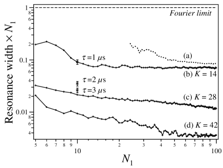
Figure 3: Temporal evolution of the width of the resonance. The numerically calculated width is multiplied by the number of kicks $N_{1}$ and plotted as a function of $N_{1}$, the total excitation time in normalized units. The Fourier limit thus corresponds to the horizontal line of ordinate 1. The solid lines (b), (c) and (d) correspond to three different values of the parameter $K$. The displayed experimental points correspond to three different values of the pulse duration $\tau=$ 1, 2 and 3 $\mu$s. The dotted line (a) corresponds to the numerical simulation using the modulated series described by Eq. (5).

In the experiment, the atomic wave packet undergoes a series of kicks separated by a free evolution. In momentum representation, a free evolution during a time $t$ amounts in multiplying the wave function by a phase factor $\exp(-i\Phi)$ with $\Phi=P^{2}t/(2\hbar_{\mathrm{eff}})$. For simplicity, consider the particular case $\varphi=0$, without loss of generality. In this case, the time interval between the last kick ($N^{th}$ kick) of the first series and the corresponding kick of the second the series is $N(r-1)/r$. The system can resolve the two frequencies if the phase evolution $\Phi$ during this interval, is of the order of one:

$$\Phi(N)=\frac{\langle P^{2}\rangle}{2\hbar_{\mathrm{eff}}}N\frac{r-1}{r}\approx 1\text{ .}$$ (6)

Before applying Eq. (6), it is important to distinguish two different regimes: (a) before the localization time, $N<N_{L}$ (where $N_{L}=t_{L}/T_{1}$), the dynamics is a classical diffusion, and $\langle P^{2}\rangle\propto N$; (b) for $N>N_{L}$ the momentum distribution is localized and $\langle P^{2}\rangle$ is roughly constant. Thus, according to Eq. (6), the resolution $(r-1)$ has a fast, unusual, decrease as $N^{-2}$ as long as $N<N_{L}$, and a slower decrease as $N^{-1}$ for $N>N_{L}$. Otherwise stated, for times $t<t_{L}$ the system takes an advance over the Fourier limit that it preserves when $t>t_{L}$. Effectively, the numerical simulations in Fig. 3 indicate that the linewidth decreases faster than the standard Fourier decrease, as $N^{-1}$. The higher resolution results, on the one hand, from the sensitivity of the quantum interference process to frequency differences, and, on the other hand, from the amplification of such sensitivity by a chaotic diffusion. The underlying physical process relies on long-range correlations in the momentum space. Breaking exact time periodicity of the excitation destroys those correlations and, as a consequence, the localization. This also suggests that the frequency resolution improves as the dynamics becomes more chaotic, as $K$ increases. Numerically, no lower limit has been found to the resolution, which can reach several orders of magnitude below the Fourier limit. There are nevertheless limits for real applications since the signal $p(P=0)$ decreases with increasing $K$, roughly like $1/K$. In our experiment, the signal/noise ratio is of the order of 100, which in principle allows widths below 1/100 of the Fourier limit. There is however an experimental imperfection: the SW waist is only about 1.6 times the size of the atomic cloud: depending on their position in the laser beam, the atoms experience different values of $K$. This leads to an inhomogeneous broadening of the resonance line, which explains the discrepancies between experimental data and the numerical simulation in Fig. 3. Improvements towards narrower sub-Fourier lines are currently under study.

A few additional remarks might be done. Firstly, sub-Fourier behavior is allowed because the resonance lines are not the direct Fourier transform of a temporal signal. Secondly, the observation of sub-Fourier lines is not limited to a specific choice of parameters. The curve displayed in Fig. 1 is the most sub-Fourier one (by a factor 35) that we have observed, but sub-Fourier widths are a standard behavior. Thirdly, since the process described here involves two frequencies, it is quite analogous to a frequency measurement by the heterodyning technique. This might be exploited for realizing ultra-fast frequency locking to a standard frequency, using $p(0)$ as an error signal, that would thus respond in a sub-Fourier time. In a completely different field, an analogy can be made between the present experiment and near field optical microscopy where details of size far below the diffraction limit can be resolved. In both cases, the resolution is obtained at the price of a signal loss.

In conclusion, we have experimentally demonstrated the possibility of using of a quantum-chaotic device to discriminate two frequencies, far below the Fourier limit. The principle relies on the sensitivity of quantum interferences to periodicity breaking, amplified by a chaotic diffusive process. No physical law has been broken, but the very widely used “rule of thumb” stating that the minimum width of a quantum resonance should be limited by the excitation time is here not valid, opening the way to a new field of quantum-chaotic signal processing.

- (1) Technically, refers to the square root of the variance of the frequency distribution, while is the square root of the variance of the temporal distribution of the signal. For most signal shapes, they can be associated with the width (at half maximum) of the frequency signal and its time duration, respectively.
- (2) N. Ramsey, Molecular beams (Clarendon Press, Oxford, 1956).
- (3) F. S. Cataliotti, R. Scheunemann, T. W. Hänsch, M. Weitz, Phys. Rev. Lett. 87, 113601 (2001).
- (4) J. Ringot, P. Szriftgiser, J. C. Garreau, and D. Delande, Phys. Rev. Lett. 85, 2741 (2000).
- (5) R. Graham, M. Schlautmann, and P. Zoller, Phys. Rev. A 45, 19 (1992).
- (6) F. L. Moore, J. C. Robinson, C. Bharucha, P. E. Williams, M. G. Raizen, Phys. Rev. Lett. 73, 2974 (1994); H. Ammann, R. Gray, I. Shvarchuck, and N. Christensen, ibid. 80, 4111 (1998); M. B. D’arcy, R. M. Godun, M. K. Oberthaler, D. Cassetari, and G. S. Summy, ibid. 87, 074102 (2001).
- (7) B. G. Klappauf, W. H. Oskay, D. A. Steck, and M. G. Raizen, Phys. Rev. Lett. 81, 1203 (1998).
- (8) See e. g. C. Cohen-Tannoudji in Fundamental Systems in Quantum Optics edt. by J. Dalibard, J. M. Raimond, and J. Zinn-Justin (North-Holland, Amsterdam, 1992); P. Meystre Atom Optics (Springer, New York, 2001).
- (9) G. Casati, B. V. Chirikov, J. Ford, and F. M. Izrailev, Lect. Notes Phys. 93, 334 (1979); F. Haake, Quantum Signatures of Chaos, edition (Springer, Berlin, 2001).
- (10) P. W. Anderson, Phys. Rev. 109, 1492 (1958) and Rev. Mod. Phys. 50, 191 (1978); S. Fishman, D. R. Grempel, and R. E. Prange, Phys. Rev. Lett. 49, 509 (1982).
- (11) M. Kasevich, D. S. Weiss, E. Riis, K. Moler, S. Kasapi, and S. Chu, Phys. Rev. Lett. 66, 2297 (1991); J. Reichel, F. Bardou, M. Ben Dahan, E. Peik, S. Rand, C. Salomon, and C. Cohen-Tannoudji, Phys. Rev. Lett. 75, 4575 (1995); J. Ringot, P. Szriftgiser, and J. C. Garreau, Phys. Rev. A 65, 013403 (2002).