Measurement of qutrits

Abstract

We proposed the procedure of measuring the unknown state of the three-level system – the qutrit, which was realized as the arbitrary polarization state of the single-mode biphoton field. This procedure is accomplished for the set of the pure states of qutrits; this set is defined by the properties of SU(2) transformations, that are done by the polarization transformers.

Quantum Electronics Division, Physics Department, Moscow State University, 119899 Moscow, Russia. e-mail:postmast@qopt.phys.msu.su

1 Introduction

In the physics of quantum information those systems that can be completely described in terms of three orthogonal states, were called qutrits (q-trit). In the case of a pure state the wave function of the three-level system can be written as:

$$\Psi=c_{1}\left|1\right\rangle+c_{2}\left|2\right\rangle+c_{3}\left|3\right\rangle,$$ (1)

where $|$1$\rangle$, $|$2$\rangle$, $|$3$\rangle$ - are the orthogonal basis states. The complex coefficients $c_{j}$ are the amplitudes of the basis states $\left|j\right\rangle$ and satisfy the following normalizing condition

$$\sum\limits_{i=1}^{3}{\left|{c_{j}}\right|^{2}}=1.$$ (2)

Decomposition (1) is the generalization of the definition of qubit when the dimension of the quantum system $d=3$.

Several ways are known how to experimentally realize the multilevel quantum optical systems. In one of them [1] the interferometric procedure of state preparation is used, when the attenuated laser pulses are sent into the multi-armed interferometer. The number of arms is equal to the system’s dimensionality. Identification of basis states is done either through the pulses delay (temporal basis) or by the presence of constructive interference in the certain arm of the interferometer that is put into the registration system (energy basis). The other example is the optical field that consists of the pairs of correlated photons that belong to the different polarization modes. The preparation of such fields and their unitary transformations are reviewed in [2,3]. Multi-level systems attract a great interest in quantum cryptography, where by using those systems one can achieve secrecy growing when the eavesdropper uses so called symmetric individual attacks [4-6].

The problem of the adequate measurement of the parameters of the quantum state is one of the major ones in quantum information science. With the decision of this problem one can expect the realization of the information’s output devices, the protocols of error correction, quantum repeaters, and other quantum communication devices. From the fundamental point of view the question of minimal set of measurements that is needed for the complete description of the system’s state is also very important. Let us notice that in some cases it is not necessary to perform a complete set of measurements to define system’s purity [7].

Of course, for different types of quantum states one also uses different types of measurement procedures. As an example for a squeezed state of light, methods of homodyne tomography are developing [8]; they, in principle allow restoring the density matrix of n-photon Fock states [9]. For the polarization-squeezed [10] and scalar [11] light the fluctuations of Stokes parameters are analyzed and the quasi-probability function is restored [12]. In the case of two-photon fields one registers the set of the fourth order field moments in different spatial and polarization modes [13]. Let us notice that in context of each experimental procedure, the a-priori information about the properties of the examined state plays an important role.

2 Biphotons as qutrits

This work is devoted to the optical realization of the protocol that allows restoring the density matrix of an unknown three-level system quantum state. The polarization state of the two-photon field that belongs to the single spatial and frequency mode is the object of our investigation. In [2] it was shown that the pure state of such a field can be written as:

$$\Psi=c_{1}\left|{2,0}\right\rangle+c_{2}\left|{1,1}\right\rangle+c_{3}\left|{0,2}\right\rangle.$$ (3)

The two-photon Fock states in two orthogonal; polarization modes H and V serve as the basis states. So, for example, the second term in (3) corresponds to the existence of one photon in modes H and V with $\left|{c_{2}}\right|^{2}$ probability. The vacuum component $\left|{0,0}\right\rangle$ is not considered in (3), because when the field is registered by the method of coincidence of photopulses, the contribution of this component to the measured correlation functions is equal to zero. The imaginary parts of the complex coefficients $c_{j}=\left|{c_{j}}\right|\exp\left\{{i\varphi_{j}}\right\},j=1,2,3$ are the phases of the basis states. The total phase of the wave function is incidental, and that’s why one of the phases can be excluded from the consideration, giving us the relative phases. For example, $\varphi_{12}=\varphi_{1}-\varphi_{2}$ and $\varphi_{32}=\varphi_{3}-\varphi_{2}$.

For the description of the polarization properties of the single-mode biphoton field, in [14] the so-called polarization or fourth-order coherency matrix was introduced:

$$K_{4}=\left({{\begin{array}[]{*{20}c}A\hfill&D\hfill&E\hfill\\ {D^{\ast}\hfill}&C\hfill&F\hfill\\ {E^{\ast}\hfill}&{F^{\ast}\hfill}&B\hfill\\ \end{array}}}\right).$$ (4)

The elements of this matrix represent the normally ordered fourth moments of the field that can be written as

$$\begin{array}[]{l}A\equiv\left\langle{a^{\dagger 2}a^{2}}\right\rangle,\quad B\equiv\left\langle{b^{\dagger 2}b^{2}}\right\rangle,\quad C\equiv\left\langle{a^{\dagger}b^{\dagger}ab}\right\rangle,\\ D\equiv\left\langle{a^{\dagger 2}ab}\right\rangle,\quad E\equiv\left\langle{a^{\dagger 2}b^{2}}\right\rangle,\quad F\equiv\left\langle{a^{\dagger}b^{\dagger}b^{2}}\right\rangle\par.\\ \end{array}$$

Here, $a^{\dagger}\equiv a_{H}^{\dagger}$, $b^{\dagger}\equiv a_{V}^{\dagger}$, $a\equiv a_{H}$, $b\equiv a_{V}$ - are the operators of photon creation and annihilation in polarization modes $H$ and $V$, respectively. It can be noticed that the diagonal components of $K_{4}$ are real. They characterize the intensity fluctuations in parallel ($A$ and $B$) or orthogonal ($C$) polarization modes. Non-diagonal elements $D$, $E$, $F$ in general case are complex.

Since the state of biphoton field can be fully described by the fourth moments of the field, the elements of $K_{4}$ matrix can be derived through the components of the density matrix of biphoton field. As an example for the pure state (3), by definition [15] $\rho_{mn}=c_{m}c_{n}^{\ast}$ and

$$\rho_{11}=\left|{c_{1}}\right|^{2}=A/2,\quad\rho_{22}=\left|{c_{2}}\right|^{2}=C,\quad\rho_{33}=\left|{c_{3}}\right|^{2}=B/2,$$ (5)

$$\rho_{12}=c_{1}c_{2}^{\ast}={D^{\ast}}/{\sqrt{2}},\quad\rho_{13}=c_{1}c_{3}^{\ast}={E^{\ast}}/2,\quad\rho_{23}=c_{2}c_{3}^{\ast}={F^{\ast}}/{\sqrt{2}}.$$ (6)

The condition of state’s purity

$$\rho^{2}=\rho.$$ (7)

And normalizing condition

$$Sp\left(\rho\right)=1$$ (8)

impose the certain constraints between the elements of $K_{4}$ matrix. Thus, from (8) it follows that

$$A+B+2C=2,$$ (9)

And condition (7) gives

$$E^{\ast}={ABC}\mathord{\left/{\vphantom{{ABC}{DF}}}\right.\kern-1.2pt}{DF},\quad\left|F\right|^{2}=BC\mbox{,}\quad\left|D\right|^{2}=C(2-B-2C).$$ (10)

For the mixed state, the definition of density matrix also includes the complementary averaging with the classical distribution function $P$ by the possible states of the system, where $P$ satisfies $\sum\limits_{i=1}{P_{i}}=1$, and the components of density matrix are:

$$\rho_{mn}=\overline{c_{m}c_{n}^{\ast}}.$$ (11)

3 Measurement of the state of qutrits

The question rises – how many (real) parameters should be measured to characterize completely the unknown state of biphoton field? From the definition and properties of the density matrix, it follows that in the case of the pure state, the number of real parameters, that define the state of the system that has a dimension $d$, is equal to $2d-2$, and in the case of a mixed state is equal to $d^{2}-1$. Correspondingly for the qutrits in the first case one needs to know four real numbers, in the second case - eight. Considering that in experiment one measures the unnormalized state’s amplitudes and conditions (8,9) are needed to be checked every time after measuring all three diagonal elements of $K_{4}$ matrix, we obtain that in pure state five moments are needed to be measured and in the mixed state - nine.

Before we go further into the discussion of suggested protocol, we notice that the measurement procedure always leads to the destruction of our state that is caused by its interaction with the classical measuring device, in our case – with the detector. So when we speak about the input state, we always have in mind that it is introduced by a large enough set of copies, and part of them can be destroyed by the measurement. The results of the measurements will be applied to the rest part of the ensemble; this procedure lies at the heart of the ensemble method of quantum measurements.

In quantum optics as the measuring apparatus for the fourth moments of the field usually serves the Brown-Twiss scheme, which consists of the beam splitter with the photo detectors in the output ports (Fig.1). Polarization transformations in each spatial mode is done with the help of retardation plates ($\lambda$/2 $\lambda$/4) and polarization filters (polarizers) . Let’s examine the normally ordered fourth moments of the field $R_{12}\left({\chi_{1},\theta_{1},\chi_{2},\theta_{2}}\right)\sim\left\langle{{b^{\prime}}_{1}^{\dagger}{b^{\prime}}_{2}^{\dagger}{b^{\prime}}_{1}{b^{\prime}}_{2}}\right\rangle$, that are registered in the scheme that is shown at Fig.1, with the given wave plates orientation and the fixed polarization that is transmitted by polarizers. Our goal will be the search of the minimal set of such moments i.e. parameters that are measured in the experiment, from which one can compose all the elements of $K_{4}$ matrix. In this case the input field will be transformed by the wave plates and polarizers in such way that the registered moments can be derived through the components of $K_{4}$ matrix. Polarization transformations that are done by the wave plates are unitary and the polarizer plays the role of the polarization filter that sets the polarization state registered by the detectors. This idea is based on the classical schemes in which the Stokes parameters are measured [16]. It was also used in [13] for the measurement of the polarization properties of the biphoton light in two spatial modes (so-called two-qubit case). Let’s notice that the choice of quarter- and half- wave plates as the polarization transformers evidently is not unique, it is dictated by the convenience (these wave plates are most commonly used in the polarization experiments) and by the clearance of the transformations.

The consecutive action of the beam splitter, two wave plates and the polaraizer that transmits the vertical polarization on the signal (idler) photon is described by the following matrix transformations:

$$\left({{\begin{array}[]{*{20}c}{a}^{\prime}\hfill\\ {b}^{\prime}\hfill\\ \end{array}}}\right)=G_{V}G_{\lambda/2}G_{\lambda/4}G_{BS}\left({{\begin{array}[]{*{20}c}a\hfill\\ b\hfill\\ \end{array}}}\right),$$ (12)

where $a$ and $b$ – are the annihilation operators of the input state in two orthogonal polarization modes $H$ and $V$ at the input, ${a}^{\prime}$ and ${b}^{\prime}$ - are the annihilation operators at the output of the transformers; the state vector is written in Jones representation.

$$G_{BS}=\left({{\begin{array}[]{*{20}c}{1\mathord{\left/{\vphantom{1{\sqrt{2}}}}\right.\kern-1.2pt}{\sqrt{2}\hfill}}&0\hfill\\ 0\hfill&{1\mathord{\left/{\vphantom{1{\sqrt{2}}}}\right.\kern-1.2pt}{\sqrt{2}\hfill}}\\ \end{array}}}\right)$$ (13)

is the matrix that describes the action of the non-polarizing beam splitter,

$$G_{V}=\left({{\begin{array}[]{*{20}c}0\hfill&0\hfill\\ 0\hfill&1\hfill\\ \end{array}}}\right)$$ (14)

is the matrix of the polarizer that transmits the vertical field component,

$$G_{\lambda/4,\lambda/2}=\left({{\begin{array}[]{*{20}c}t\hfill&r\hfill\\ {-r^{\ast}\hfill}&{t^{\ast}\hfill}\\ \end{array}}}\right)$$ (15)

are the matrices of the wave plates. Here coefficients $t$ and $r$ are equal to

$$\begin{array}[]{l}t=\cos\delta+i\sin\delta\cos 2\alpha,\\ r=i\sin\delta\sin 2\alpha,\\ \end{array}$$ (16)

where $\delta$ - is the optical thickness, and $\alpha$ - is the angle between optical axis and the vertical direction ($V)$. For the quarter and half- wave plates $\delta_{\lambda/4}=\pi/4,\quad\alpha_{\lambda/4}\equiv\chi,\quad\delta_{\lambda/2}=\pi/2\,\quad\alpha_{\lambda/2}\equiv\theta,$ and these coefficients can be rewritten as:

$$\begin{array}[]{l}t_{\lambda/4}=1\mathord{\left/{\vphantom{1{\sqrt{2}}}}\right.\kern-1.2pt}{\sqrt{2}}(1+i\cos 2\chi),\\ r_{\lambda/4}=i\mathord{\left/{\vphantom{i{\sqrt{2}}}}\right.\kern-1.2pt}{\sqrt{2}}\sin 2\chi,\\ \end{array}$$ (17)

$$\begin{array}[]{l}t_{\lambda/2}=i\cos 2\theta,\\ r_{\lambda/2}=i\sin 2\theta.\\ \end{array}$$ (18)

It is clearly seen from the definition of $K_{4}$ matrix how one can measure its diagonal components or moments $A,B$ and $C$. In the first case the optical axes of all wave plates are set vertically - along the direction of the transmission of polarizer $P$. In the second case the polarization in two arms must be rotated by 90⁰, that is achieved by setting $\chi_{1}=0^{o},\theta_{1}=45^{o}$, $\chi_{2}=0^{o},\theta_{2}=45^{o}$. In the third case the polarization is rotated only in one arm, and according to scheme’s symmetry it is not important in which. The set is: $\chi_{1}=0^{o},\theta_{1}=45^{o}$, $\chi_{2}=0^{o},\theta_{2}=0^{o}$. The more complex transformations are needed when non-diagonal components of $K_{4}$ matrix are measured. As an example let’s look how the following setting of elements acts on the input state does. Let $\chi_{1}=0^{o},\theta_{1}=45^{o}$, $\chi_{2}=45^{o},\theta_{2}=22.5^{o}$. It is not hard to calculate that in this case

$$\begin{array}[]{l}R_{12}=\left\langle{{b^{\prime}}_{1}^{\dagger}{b^{\prime}}_{2}^{\dagger}{b^{\prime}}_{1}{b^{\prime}}_{2}}\right\rangle=1\mathord{\left/{\vphantom{18}}\right.\kern-1.2pt}8\left[{\left\langle{a^{{\dagger}2}a^{2}}\right\rangle-\left\langle{a^{{\dagger}2}ab}\right\rangle-\left\langle{a^{\dagger}b^{\dagger}a^{2}}\right\rangle+\left\langle{a^{\dagger}b^{\dagger}ab}\right\rangle}\right]=\\ 1\mathord{\left/{\vphantom{18}}\right.\kern-1.2pt}8\left[{A+C-2ReD}\right].\\ \end{array}$$ (19)

The measured moment in this case contains the contributions from three elements of the coherency matrix. Two of them are real diagonal components $A$, $C$ . The third one is the real part of the (complex) non-diagonal element $D$. This example shows that since we are not directly measuring the phases of the states $\varphi_{1}$, $\varphi_{2}$ or $\varphi_{3}$, but its cosine and sine, then the number of the measurements needed is increasing. In the real experiment, which description is shown below, in each arm of the Brown-Twiss scheme we used simpler configuration than the set of two rotating wave plates and the fixed polarizer. We considered the fact that when measuring the moments of the fourth order, the transformation that is done by the half wave plate and the fixed polarizer is equivalent to the action of one polarizer, which orientation is given by the angle $\beta$. The rotation angles of half wave plate $\theta$ and the polarizer $\beta$ are bounded by the equation:

$$\beta=-2\theta.$$ (20)

In the Table 1 we show the values of the orientation angles of the quarter wave plates ($\chi_{1,2})$ and polarizers $(\beta_{1,2})$ in two arms versus the value of the corresponding measured moment. This table essentially serves as the protocol of the reconstruction of the input state of the field that is presented by the biphoton-qutrit. It can be seen that in general case, the number of required measurements is equal to nine. First seven measurements realize the protocol for the pure input state. Two additional measurements are necessary for the definition of the cosine (sine) values of the corresponding phases. Eighth and ninth lines of the table show how to find the real and imaginary parts of the complex moment , which in the case of the pure state, according to (10), is derived through the rest of the moments. Let’s notice that in our protocol for the definition of each non-diagonal elements of $K_{4}$ matrix, only three moments must be known, what the minimal number of measurement needed is apparently.

Table 1: The protocol of measurement of the moment set, which form the coherency matrix.

	plate $\lambda/4$	Polarizer	plate $\lambda/4$	Polarizer	Field
	(I)	(I)	(II)	(II)	Moment
	$\chi_{1}$, deg.	$\beta_{1}$, deg.	$\chi_{2}$, deg.	$\beta_{2}$, deg.
1.	0	90	0	90	A/4
2.	0	90	0	0	C/4
3.	0	0	0	0	B/4
4.	45	0	0	0	1/8(B+C+2ImF)
5.	45	-45	0	0	1/8(B+C-2ReF)
6.	45	-45	0	90	1/8(A+C-2ReD)
7.	45	0	0	90	1/8(A+C+2ImD)
8.	-45	22,5	-45	22,5	1/16(A+C-2ImE)
9.	45	45	45	-45	1/16(A+C-2ReE)

4 Experiment

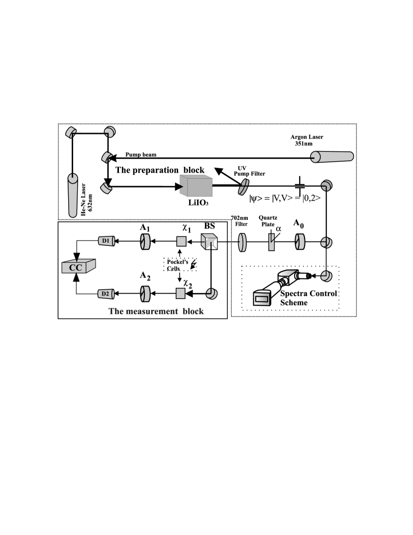
Figure 2: Experimental setup.

The experimental setup is shown at Fig.2. It can be conventionally separated in two blocks – the block of the preparation of the input state and the block of measurements. First block includes the cw Ar⁺ laser, operating at 351 nm, with the output power of 120 mW, which serves as the pump for the non-linear lithium iodate crystal, where the process of biphoton generation goes on. This block also includes the system of adjustment mirrors, quartz wave plate, which orientation could be smoothly varied, and the interference filter with the central wavelength of 702 nm, and 5 nm FWHM. Two-photon states of light were generated by the process of spontaneous parametric down-conversion (SPDC) inside the non-linear crystal. We used type-I collinear, frequency degenerate SPDC. The wavelength of biphoton radiation was $\lambda_{s}=\lambda_{i}=2\lambda_{p}=702\pm 9nm$. The polarization of both photons was vertical. In this case, right after the crystal, the biphoton field was in state

$$\Psi=c_{3}^{in}\left|{0,2}\right\rangle+\left|{vac}\right\rangle.$$ (21)

The quartz wave plate was used to transform this state to the one that is described by equation (3) (Fig.2). It is known that all the transformations that are done with the polarization of biphotons by the retardation plates can be described by the unitary (3$\times$3) matrices G [2]:

$$\left({{\begin{array}[]{*{20}c}{c_{1}\hfill}\\ {c_{2}\hfill}\\ {c_{3}\hfill}\\ \end{array}}}\right)^{out}=G\left({{\begin{array}[]{*{20}c}{c_{1}\hfill}\\ {c_{2}\hfill}\\ {c_{3}\hfill}\\ \end{array}}}\right)^{in},$$ (22)

where

$$G=G\left({\delta,\alpha}\right)=\left(\begin{array}[]{ccc}t^{2}&\sqrt{2}tr&r^{2}\\ -\sqrt{2}tr^{\ast}&\left|t\right|^{2}-\left|r\right|^{2}&\sqrt{2}t^{\ast}r\\ r^{\ast 2}&{-\sqrt{2}}t^{\ast}r^{\ast}&t^{\ast 2}\end{array}\right),$$ (23)

and coefficients $t$ and $r$ were introduced by (16).

Matrices (23) give us the irreducible presentation of SU(2) group with 3$\times$3 dimensionality in the space of the state vectors (3). Let’s notice that one cannot realize an arbitrary polarization state of a biphoton field, by using wave plates only. In general case such transformations, together with the space of a state vectors (3) form the three-dimensional unitary presentation of SU(3) group.

The thickness of the setting wave plate was $h$= 824$\pm$1mkm, therefore the parameter $\delta\equiv\frac{\pi}{\lambda}\left({n_{o}-n_{e}}\right)h$ was fixed. The second parameter $\alpha$ was changing during the experiment that allowed us to set the state of a biphoton field that was given onto the input of the measurement block. It is clear that all the states that were prepared in such a way did not drive our biphoton field out of the pure states class.

The measurement block consists of the Brown-Twiss scheme that is shown at Fig.1. In our experiments we used Pockel cells instead of the quarter wave plates. The use of the Pockel cells seemed preferable to us, because it allowed controlling the polarization transformation distantly, by applying the certain voltages on them. The spectral control of the biphoton field was realized with the help of the spectrograph. Pulses coming from the detectors were driven onto the standard coincidence scheme, which measured the number of coincidences rate that is proportional to correlators (19).

The measurement procedure was as follows. For the certain orientation of the setting wave plate, we performed a set of measurements that is described in Table 1. Then we rotated the setting wave plate by $\alpha$, what corresponded to the change of the input state, and performed the same set of measurements.

The dependence of modulo squared of the three state’s amplitude and two phases from the rotation angle of a setting wave plate is plotted on Fig.3-6. Each experimental dot on the plot corresponds to the certain input state that is given by a setting wave plate. Solid lines – result of theoretical calculations by formulas (22,23). Since all three measured moments contributed to the phase’s calculation (look at Table 1); the errors of three measurements were added and the precision of a corresponding measurement was low. The main source of errors is the low quality of the Pockel cells and as a consequence – the inadequacy of the polarization transformations that are done with these elements. Definitely by using the retardation wave plates that are working in zero-order interference regime is the only way to overcome this problem. We notion the good correspondence of the calculations and the experimental results when measuring the modules of state’s amplitudes. All errors that appear here are due to the errors in setting the correct polarizer orientation angle.

The presentation of the measured field states in terms of complex coefficients $c_{j}$ as it is done on Fig.3-6, is possible only for the pure states. For the mixed states, one needs to measure all six moments, that form the $K_{4}$ (4) matrix. The real and imaginary parts of the moments $D$ and $F$ are shown at Fig.7,8. The calculated and measured components of density matrix of the state that correspond to the orientation of the setting wave plate by $\alpha=25^{0}$, are shown at Fig. 9. Of course, for the pure states, which case was realized in our experiment, these moments can be derived through amplitudes $c_{i}$. Moment was not measured in this case, because as it is shown above, it could be derived through the other moments.

5 Conclusion

In this work, we proposed the procedure of measuring the unknown state of the three-level system – the qutrit, which was realized as the arbitrary polarization state of the single-mode biphoton field. This procedure is experimentally realized for the set of the pure states of qutrits; this set is defined by the properties of SU(2) transformations, that are done by the polarization transformers (retardation plates).

However, it seems to be interesting to realize the complete protocol of density matrix restoration both for the pure and for the mixed states of qutrits. These experiments are now in progress and their results will be published soon. Separately, the question of maximum-likelihood estimation of the experimental results to the most probable quantity of $\rho$ [13,17] will be reviewed.

This work was done by the financial support of RFBR (grant # 02-02-16664) and INTAS (01-2122).

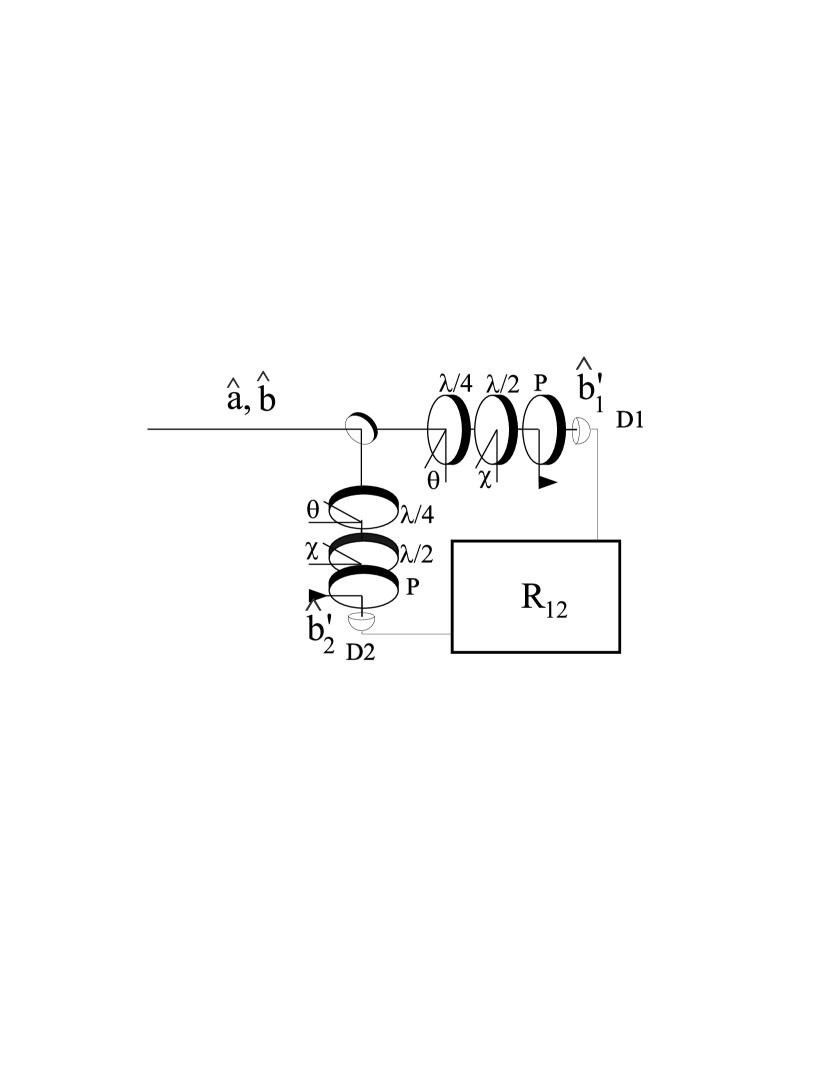
Figure 1: Brown-Twiss scheme in which one can measure the moments that form the coherency matrix $K_{4}$. BS – beam splitter, RP – retardation plates of quarter and half wavelength, that are characterized by the parameters $\delta_{\lambda/2},\delta_{\lambda/4}$ and $\theta_{\lambda/2},\chi_{\lambda/4}$, P are the polarizers that transmit the vertical polarization.

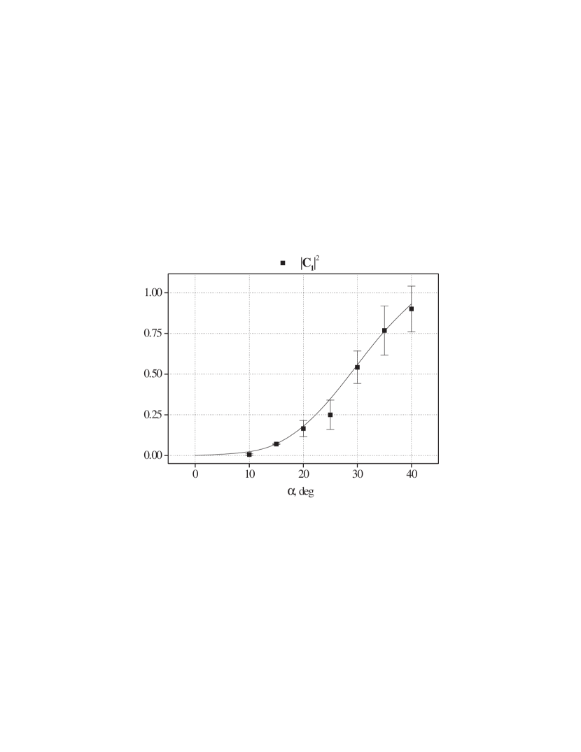
Figure 3: Dependence of the parameter of the input state $\left|{c_{1}}\right|^{2}$,from the rotation angle of the setting retardation plate

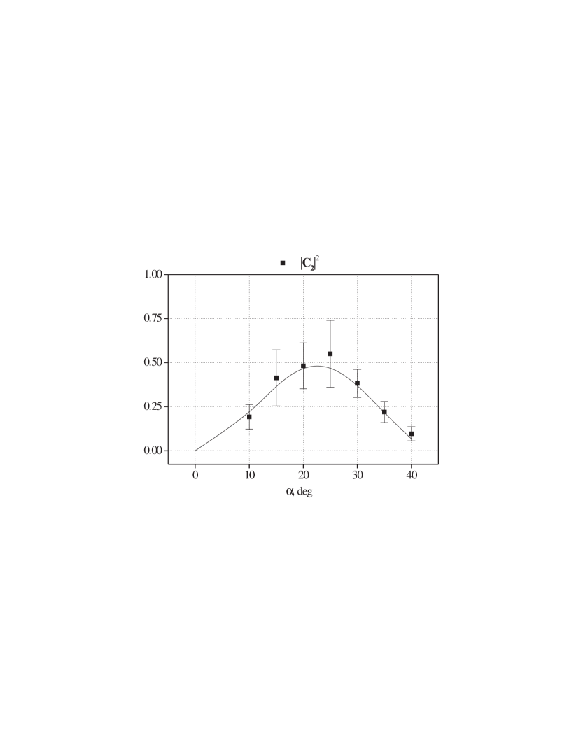
Figure 4: Dependence of the parameter of the input state $\left|{c_{2}}\right|^{2}$,from the rotation angle of the setting retardation plate

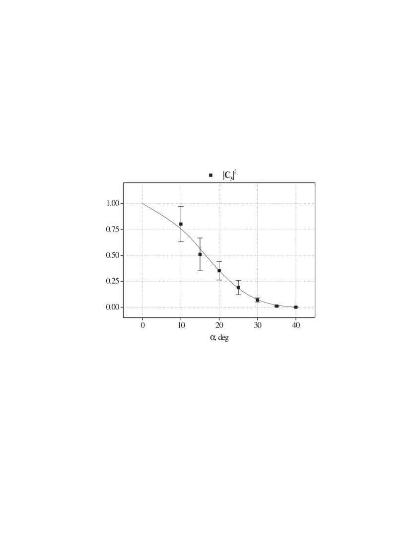
Figure 5: Dependence of the parameter of the input state $\left|{c_{3}}\right|^{2}$,from the rotation angle of the setting retardation plate

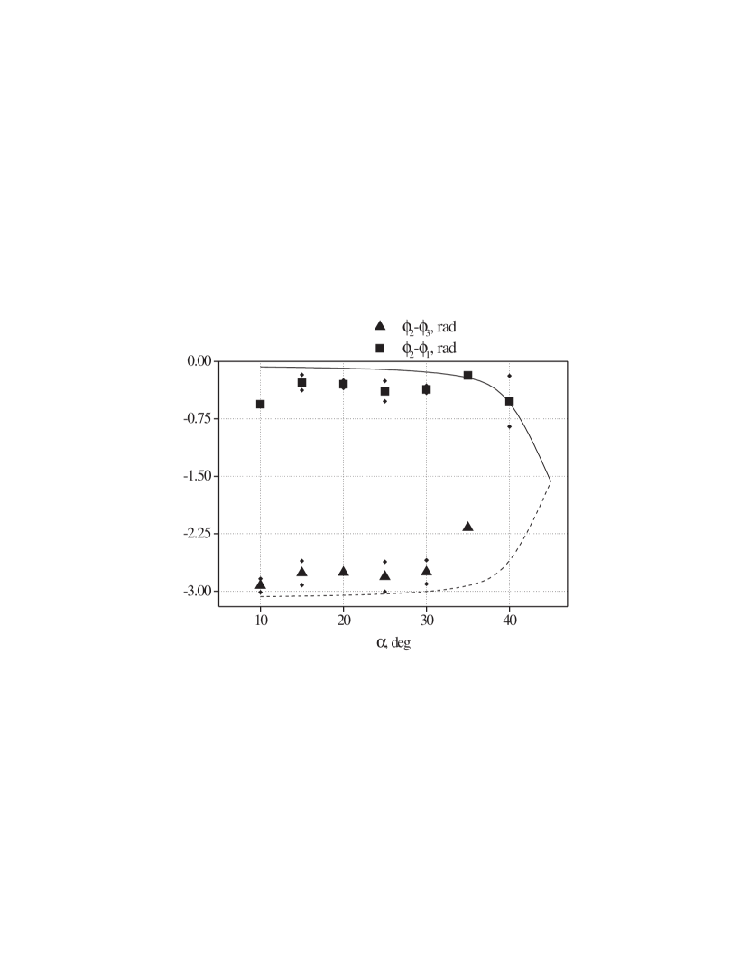
Figure 6: Dependence of the parameter of the input state $\varphi_{2}-\varphi_{3},\varphi_{2}-\varphi_{1}$, from the rotation angle of the setting retardation plate

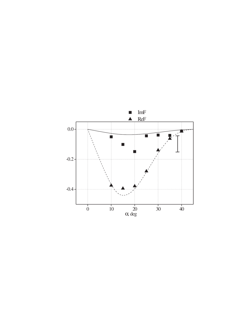
Figure 7: Dependencies of the real and imaginary parts of the moment F from the rotation angle of the setting retardation plate.

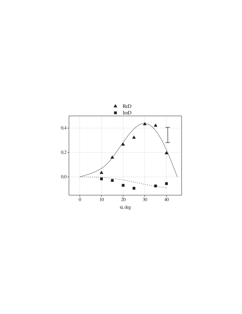
Figure 8: Dependencies of the real and imaginary parts of the moment D from the rotation angle of the setting retardation plate.

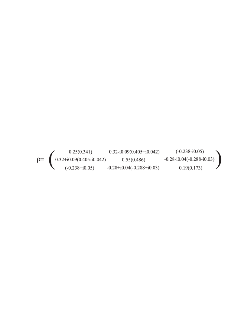
Figure 9: Density matrix that is measure for the input state given by the angle of the setting wave plate $\alpha=25^{0}$. Theoretically calculated values are placed in brackets.

References

- [1] H.Bechmann-Pasquinucci and W.Tittel, Phys.Rev.A, 51, 062308 (2000).
- [2] A.V. Burlakov, D.N. Klyshko, Pis’ma JETP 69, 11, 795 (1999).
- [3] A.V.Burlakov, M.V.Chekhova, O.A.Karabutova, D.N.Klyshko, and S.P.Kulik, Phys. Rev. A 60, No 6, R4209 (1999).
- [4] H.Bechmann-Pasquinucci and A.Peres, Phys.Rev.Lett. 85 (13), 3313 (2000).
- [5] N.J.Cerf, M.Bourennane, A.Karlsson, and N.Gisin, Phys.Rev.Lett., 88 (11), 127902 (2002).
- [6] D.Bruss and C.Macchiavello, Phys.Rev.Lett., 88 (11), 127901 (2002).
- [7] A.K.Ekert, C.M.Alves, D.K.L.Oi, M.Horodecki, P.Horodecki, and L.C.Kwek, Phys. Rev. Lett. 88, 217901 (2002).
- [8] G.M.D’Ariano, in Quantum Optics and Spectroscopy of Solids, edited by A.S.Shumowsky and T.Hakiouglu (Kluwer, Amsterdam), 175 (1997).
- [9] S.Schiller, G.Breitenbach, S.F.Pereira, T.Muller, and J.Mlynek, Phys.Rev.Lett., 77 (12), 2933 (1996).
- [10] A.S. Chirkin, A.A. Orlov, D.Yu. Parashuk, Quantum Electronics, 20, 999 (1993).
- [11] V.P. Karassev, J. Sov. Laser Res. 12, No 5, 147 (1991).
- [12] A.V. Masalov, V.P. Karassev. Optics and Spectroscopy, 91 (4), 558 (2001).
- [13] D.James, P.Kwiat, W.Munro, and A.White, Phys. Rev. A, 64, 052312 (2001).
- [14] D.N. Klyshko. JETP, 111, 6, 1955-1983 (1997).
- [15] L.D. Landau, E.M. Lifshitz. Quantum Mechanics, 1967.
- [16] W. Shurkliff. Polarized light. Production and use. Harvard Univ. Press, 1962.
- [17] G.M.D’Ariano, M.G.A.Paris, and M.F.Sachi, Phys.Rev.A, 62, 023815 (2000).