Five Lectures On Dissipative Master Equations

Five Lectures On Dissipative Master Equations

Introductory Remarks

The damped harmonic oscillator is arguably the simplest open quantum system worth studying. It is also of great practical importance because it is an essential ingredient in the theoretical description of many quantum-optical experiments. One can assume rather safely that the quantum master equation of the simple harmonic oscillator wouldn’t be studied so extensively if it didn’t play such a central role in the quantum theory of lasers and the masers. Not surprisingly, then, all major textbook accounts of theoretical quantum optics DMEref:1a ; DMEref:1b ; DMEref:1c ; DMEref:1d ; DMEref:1e ; DMEref:1f ; DMEref:1g ; DMEref:1h ; DMEref:1i ; DMEref:1j ; DMEref:1k ; DMEref:1l ; DMEref:1m ; DMEref:1n ; DMEref:1o contain a fair amount of detail about damped harmonic oscillators. Fock state representations or phase space functions of some sort are invariably employed in these treatments.

The algebraic methods on which we’ll focus here are quite different. They should be regarded as a supplement of, not as a replacement for, the traditional approaches. As always, every method has its advantages and its drawbacks: a particular problem can be technically demanding in one approach, but quite simple in another. This is, of course, also true for the algebraic method. We’ll illustrate its technical power by a few typical examples for which the standard approaches would be quite awkward.

1 First Lecture: Basics

The evolution of a simple damped harmonic oscillator is governed by the master equation

$$\frac{\partial}{\partial t}\varrho_{t}={\rm i}\omega[\varrho_{t},a^{\dagger}a] - \frac{1}{2}A(\nu+1)\left(a^{\dagger}a\varrho_{t}-2a\varrho_{t}a^{\dagger}+\varrho_{t}a^{\dagger}a\right)$$ (1)

$$- \frac{1}{2}A\nu\left(aa^{\dagger}\varrho_{t}-2a^{\dagger}\varrho_{t}a+\varrho_{t}aa^{\dagger}\right)\;,$$

where $a^{\dagger},a$ are the ladder operators of the oscillator; $\omega$ is its natural (circular) frequency; $A$ is the energy decay rate; and $\nu$ is the number of thermal excitations in the steady state that the statistical operator $\varrho_{t}\equiv\varrho_{t}\bigl{(}a^{\dagger},a\bigr{)}$ approaches for very late times $t$. We’ll have much to say about the properties of the solutions of (1), but first we’d like to give a physical derivation of this equation.

1.1 Physical Derivation of the Master Equation

Figure 1: A two-level atom traverses a high-quality cavity, coupling resonantly to a privileged photon mode of the cavity. Prior to the interaction, there is some initial photon state in the resonator and the atom is either in the upper state of the pertinent transition (on the left) or in the lower state (on the right). After the interaction, the transition degree of the atom and the photon degree of the cavity are entangled

For this purpose we consider the following model. The oscillator is a mode of the quantized radiation field of an ideal resonator, so that excitations of this mode (vulgo photons) would stay in the resonator forever. In reality they have a finite lifetime, of course, and we describe this fact by letting the photons interact with atoms that pass through the resonator. As is depicted in Fig. 1, these atoms are also of the simplest kind conceivable: they only have two levels which – another simplification – are separated in energy by $\hbar\omega$, the energy per photon in the privileged resonator mode. Incident atoms in the upper level (symbolically: ) will have a chance to deposit energy into the resonator, while those in the lower level ( ) will tend to remove energy.

The evolution of the interacting atom-photon system is governed by the Hamilton operator

$$H=\hbar\omega a^{\dagger}a+\hbar\omega\sigma^{\dagger}\sigma-\hbar g(\sigma a^{\dagger}+\sigma^{\dagger}a)\;,$$ (2)

which goes with the name “resonant Jaynes–Cummings interaction in the rotating-wave approximation” in the quantum-optical literature. It applies as long as the atom is inside the resonator and is replaced by

$$H_{\mathrm{free}}=\hbar\omega a^{\dagger}a+\hbar\omega\sigma^{\dagger}\sigma$$ (3)

before and after the period of interaction. Here $\sigma^{\dagger}$ and $\sigma$ are the atomic ladder operators,

$$\sigma^{\dagger}=|\raisebox{-1.8pt}{\parbox[b]{10.0pt}{\begin{picture}(10.0,8.0)(0.0,-1.8)\put(0.0,-1.8){\put(1.0,2.0){\line(1,0){8.0}}\put(1.0,6.0){\line(1,0){8.0}}\put(5.0,6.0){\circle*{2.5}}}\end{picture}}}\rangle\langle\raisebox{-1.8pt}{\parbox[b]{10.0pt}{\begin{picture}(10.0,8.0)(0.0,-1.8)\put(0.0,-1.8){\put(1.0,2.0){\line(1,0){8.0}}\put(1.0,6.0){\line(1,0){8.0}}\put(5.0,2.0){\circle*{2.5}}}\end{picture}}}|\mathrel{\widehat{=}}\left(\begin{array}[]{cc}0&1\\[0.0pt] 0&0\end{array}\right)\;,\qquad\sigma=|\raisebox{-1.8pt}{\parbox[b]{10.0pt}{\begin{picture}(10.0,8.0)(0.0,-1.8)\put(0.0,-1.8){\put(1.0,2.0){\line(1,0){8.0}}\put(1.0,6.0){\line(1,0){8.0}}\put(5.0,2.0){\circle*{2.5}}}\end{picture}}}\rangle\langle\raisebox{-1.8pt}{\parbox[b]{10.0pt}{\begin{picture}(10.0,8.0)(0.0,-1.8)\put(0.0,-1.8){\put(1.0,2.0){\line(1,0){8.0}}\put(1.0,6.0){\line(1,0){8.0}}\put(5.0,6.0){\circle*{2.5}}}\end{picture}}}|\mathrel{\widehat{=}}\left(\begin{array}[]{cc}0&0\\[0.0pt] 1&0\end{array}\right)\;,$$ (4)

and $g$ is the so-called Rabi frequency, the measure of the interaction strength. Note that $\sigma^{\dagger}\sigma$ and $\sigma\sigma^{\dagger}$ project to the upper and lower atomic states,

$$\sigma^{\dagger}\sigma=|\raisebox{-1.8pt}{\parbox[b]{10.0pt}{\begin{picture}(10.0,8.0)(0.0,-1.8)\put(0.0,-1.8){\put(1.0,2.0){\line(1,0){8.0}}\put(1.0,6.0){\line(1,0){8.0}}\put(5.0,6.0){\circle*{2.5}}}\end{picture}}}\rangle\langle\raisebox{-1.8pt}{\parbox[b]{10.0pt}{\begin{picture}(10.0,8.0)(0.0,-1.8)\put(0.0,-1.8){\put(1.0,2.0){\line(1,0){8.0}}\put(1.0,6.0){\line(1,0){8.0}}\put(5.0,6.0){\circle*{2.5}}}\end{picture}}}|\mathrel{\widehat{=}}\left(\begin{array}[]{cc}1&0\\[0.0pt] 0&0\end{array}\right)\;,\qquad\sigma\sigma^{\dagger}=|\raisebox{-1.8pt}{\parbox[b]{10.0pt}{\begin{picture}(10.0,8.0)(0.0,-1.8)\put(0.0,-1.8){\put(1.0,2.0){\line(1,0){8.0}}\put(1.0,6.0){\line(1,0){8.0}}\put(5.0,2.0){\circle*{2.5}}}\end{picture}}}\rangle\langle\raisebox{-1.8pt}{\parbox[b]{10.0pt}{\begin{picture}(10.0,8.0)(0.0,-1.8)\put(0.0,-1.8){\put(1.0,2.0){\line(1,0){8.0}}\put(1.0,6.0){\line(1,0){8.0}}\put(5.0,2.0){\circle*{2.5}}}\end{picture}}}|\mathrel{\widehat{=}}\left(\begin{array}[]{cc}0&0\\[0.0pt] 0&1\end{array}\right)\;,$$ (5)

respectively.

The interaction term in (2) is a multiple of the coupling operator

$$\gamma=a\sigma^{\dagger}+a^{\dagger}\sigma$$ (6)

and $H_{\mathrm{free}}$ is essentially the square of $\gamma$ since

$$\gamma^{2}=a^{\dagger}a+\sigma^{\dagger}\sigma\;.$$ (7)

So (2) and (3) can be rewritten as

$$H=\hbar\omega\gamma^{2}-\hbar g\gamma\;,\qquad H_{\mathrm{free}}=\hbar\omega\gamma^{2}\;.$$ (8)

That $H$ commutes with $H_{\mathrm{free}}$ and both are just simple functions of $\gamma$ will enable us to solve the equations of motion quite explicitly without much effort.

We denote by $\varrho_{t}$ the statistical operator describing the combined atom-cavity system. It is a function of the dynamical variables $a^{\dagger}$, $a$, $\sigma^{\dagger}$, $\sigma$ and has also a parametric dependence on $t$, indicated by the subscript,

$$\varrho_{t}=\varrho_{t}\bigl{(}a^{\dagger}(t),a(t),\sigma^{\dagger}(t),\sigma(t)\bigr{)}\;.$$ (9)

Since a statistical operator has no total time dependence, Heisenberg’s equation of motion,

$$0=\frac{\mathrm{d}}{\mathrm{d}t}\varrho_{t}=\frac{\partial}{\partial t}\varrho_{t}-\frac{{\rm i}}{\hbar}\bigl{[}\varrho_{t},H\bigr{]}\;,$$ (10)

becomes von Neumann’s equation for the parametric time dependence,

$$\frac{\partial}{\partial t}\varrho_{t}=\frac{{\rm i}}{\hbar}[\varrho_{t},H]\;.$$ (11)

Now suppose that $t$ is the instant at which the atom enters the cavity; then it emerges at time $t+\tau$, and we have

$$\varrho_{t+\tau}=\,\mathrm{e}^{\mbox{\footnotesize$-\frac{{\rm i}}{\hbar}H\tau$}}\varrho_{t}\,\mathrm{e}^{\mbox{\footnotesize$\frac{{\rm i}}{\hbar}H\tau$}}=\,\mathrm{e}^{\mbox{\footnotesize$-\frac{{\rm i}}{\hbar}H_{\mathrm{free}}\tau$}}\left[\,\mathrm{e}^{\mbox{\footnotesize${\rm i}\phi\gamma$}}\varrho_{t}\,\mathrm{e}^{\mbox{\footnotesize$-{\rm i}\phi\gamma$}}\right]\,\mathrm{e}^{\mbox{\footnotesize$\frac{{\rm i}}{\hbar}H_{\mathrm{free}}\tau$}}$$ (12)

after we use (8) and introduce the abbreviation $\phi=g\tau$. This phase $\phi$ is the accumulated Rabi angle and, for atoms moving classically through the cavity of length $L$ with constant velocity $v$, we have $\tau=L/v$ and $\phi=gL/v$; see Fig. 2.

Figure 2: An atom takes time $\tau=L/v$ to traverse a cavity of length $L$ at speed $v$

Clearly, the $[\dots]$ term in (12) accounts for the net effect of the interaction, that part of the evolution that happens in addition to the free evolution generated by $H_{\mathrm{free}}$. We have

$$\,\mathrm{e}^{\mbox{\footnotesize${\rm i}\phi\gamma$}}=\cos\left(\phi\gamma\right)+{\rm i}\sin\left(\phi\gamma\right)=\cos\left(\phi\sqrt{\gamma^{2}}\right)+{\rm i}\gamma\frac{\sin\left(\phi\sqrt{\gamma^{2}}\right)}{\sqrt{\gamma^{2}}}\;,$$ (13)

which is just saying that the cosine is an even function and the sine is odd. Further we note that the identities

$$\begin{array}[b]{rcl}F\left({\gamma^{2}}\right)&=&\sigma^{\dagger}\sigma F\left({aa^{\dagger}}\right)+\sigma\sigma^{\dagger}F\left({a^{\dagger}a}\right)\;,\\[4.30554pt] \gamma F\left({\gamma^{2}}\right)&=&\sigma a^{\dagger}F\left({aa^{\dagger}}\right)+F\left({aa^{\dagger}}\right)a\sigma^{\dagger}\end{array}$$ (14)

hold for all functions $F\bigl{(}{\gamma^{2}}\bigr{)}$. They are immediate implications of familiar relations such as $af(a^{\dagger}a)=f(aa^{\dagger})a$, $\sigma f(\sigma^{\dagger}\sigma)=\sigma f(1)$, and $\sigma^{\dagger}f(\sigma^{\dagger}\sigma)=\sigma^{\dagger}f(0)$. We use (13) and (14) to arrive at

$$\,\mathrm{e}^{\mbox{\footnotesize${\rm i}\phi\gamma$}} = \sigma^{\dagger}\sigma\cos\left(\phi\sqrt{aa^{\dagger}}\,\right)+\sigma\sigma^{\dagger}\cos\left(\phi\sqrt{a^{\dagger}a}\,\right)$$ (15)

$$\mbox{}+{\rm i}\sigma a^{\dagger}\frac{\sin\left(\phi\sqrt{aa^{\dagger}}\,\right)}{\sqrt{aa^{\dagger}}}+{\rm i}\frac{\sin\left(\phi\sqrt{aa^{\dagger}}\,\right)}{\sqrt{aa^{\dagger}}}a\sigma^{\dagger}\;.$$

In terms of the $2\times 2$ matrix representation for the $\sigma$’s that is suggested in (4) and (5), this has the compact form

$$\,\mathrm{e}^{\mbox{\footnotesize${\rm i}\phi\gamma$}}\mathrel{\widehat{=}}\left(\begin{array}[]{cc}C&{\rm i}S^{\dagger}\\[0.0pt] {\rm i}S&\widetilde{C}\end{array}\right)$$ (16)

with the photon operators

$$C=\cos\left(\phi\sqrt{aa^{\dagger}}\,\right)\;,\qquad\widetilde{C}=\cos\left(\phi\sqrt{a^{\dagger}a}\,\right)\;,\qquad S=a^{\dagger}\frac{\sin\left(\phi\sqrt{aa^{\dagger}}\,\right)}{\sqrt{aa^{\dagger}}}\;,$$ (17)

and the adjoint of (16) reads

$$\,\mathrm{e}^{\mbox{\footnotesize$-{\rm i}\phi\gamma$}}\mathrel{\widehat{=}}\left(\begin{array}[]{cc}C&-{\rm i}S^{\dagger}\\[0.0pt] -{\rm i}S&\widetilde{C}\end{array}\right)\;.$$ (18)

We use these results for calculating the net effect of the interaction with one atom on the statistical operator $\varrho^{(\mathrm{ph})}$ of the photon state. Initially the total state $\varrho_{t}=\varrho_{t}^{\rm(ph)}\varrho_{t}^{\rm(at)}$ is not entangled, it is a product of the statistical operators referring respectively to the photons by themselves and the atom by itself. At the final instant $t+\tau$, we get $\varrho_{t+\tau}^{\mathrm{(ph)}}$ by tracing over the two-level atom,

$$\varrho_{t+\tau}^{\rm(ph)}=\,\mathrm{Tr}_{\mathrm{at}}\left\{\varrho_{t+\tau}\right\}=\,\mathrm{e}^{\mbox{\footnotesize$-{\rm i}\omega\tau a^{\dagger}a$}}\,\mathrm{Tr}_{\mathrm{at}}\left\{\,\mathrm{e}^{\mbox{\footnotesize${\rm i}\phi\gamma$}}\varrho^{(\mathrm{ph})}_{t}\varrho^{(\mathrm{at})}_{t}\,\mathrm{e}^{\mbox{\footnotesize$-{\rm i}\phi\gamma$}}\right\}\,\mathrm{e}^{\mbox{\footnotesize${\rm i}\omega\tau a^{\dagger}a$}}\;.$$ (19)

To proceed further we need to specify the initial atomic state $\varrho_{t}^{(\mathrm{at})}$, and for the present purpose the two situations of Fig. 1 will do.

On the left of Fig. 1 we have atoms arriving,

$$\varrho^{(\mathrm{at})}_{t}=|\raisebox{-1.8pt}{\parbox[b]{10.0pt}{\begin{picture}(10.0,8.0)(0.0,-1.8)\put(0.0,-1.8){\put(1.0,2.0){\line(1,0){8.0}}\put(1.0,6.0){\line(1,0){8.0}}\put(5.0,6.0){\circle*{2.5}}}\end{picture}}}\rangle\langle\raisebox{-1.8pt}{\parbox[b]{10.0pt}{\begin{picture}(10.0,8.0)(0.0,-1.8)\put(0.0,-1.8){\put(1.0,2.0){\line(1,0){8.0}}\put(1.0,6.0){\line(1,0){8.0}}\put(5.0,6.0){\circle*{2.5}}}\end{picture}}}|=\sigma^{\dagger}\sigma\mathrel{\widehat{=}}\left(\begin{array}[]{cc}1&0\\ 0&0\end{array}\right)=\left(\begin{array}[]{c}1\\ 0\end{array}\right)(1,0)\;,$$ (20)

and (19) tells us that

$$\varrho_{t+\tau}^{\mathrm{(ph)}} = \,\mathrm{e}^{\mbox{\footnotesize$-{\rm i}\omega\tau a^{\dagger}a$}}\,\mathrm{Tr}_{2\times 2}\left\{\left(\begin{array}[]{c}C\\ {\rm i}S\end{array}\right)\varrho_{t}^{(\mathrm{ph})}(C,-{\rm i}S^{\dagger})\right\}\,\mathrm{e}^{\mbox{\footnotesize${\rm i}\omega\tau a^{\dagger}a$}}$$ (23)

$$= \,\mathrm{e}^{\mbox{\footnotesize$-{\rm i}\omega\tau a^{\dagger}a$}}\left(C\varrho_{t}^{(\mathrm{ph})}C+S\varrho_{t}^{(\mathrm{ph})}S^{\dagger}\right)\,\mathrm{e}^{\mbox{\footnotesize${\rm i}\omega\tau a^{\dagger}a$}}\;.$$ (24)

Likewise, in the situation on the right-hand side of Fig. 1 we have

$$\varrho^{(\mathrm{at})}_{t}=|\raisebox{-1.8pt}{\parbox[b]{10.0pt}{\begin{picture}(10.0,8.0)(0.0,-1.8)\put(0.0,-1.8){\put(1.0,2.0){\line(1,0){8.0}}\put(1.0,6.0){\line(1,0){8.0}}\put(5.0,2.0){\circle*{2.5}}}\end{picture}}}\rangle\langle\raisebox{-1.8pt}{\parbox[b]{10.0pt}{\begin{picture}(10.0,8.0)(0.0,-1.8)\put(0.0,-1.8){\put(1.0,2.0){\line(1,0){8.0}}\put(1.0,6.0){\line(1,0){8.0}}\put(5.0,2.0){\circle*{2.5}}}\end{picture}}}|=\sigma\sigma^{\dagger}\mathrel{\widehat{=}}\left(\begin{array}[]{cc}0&0\\ 0&1\end{array}\right)=\left(\begin{array}[]{c}0\\ 1\end{array}\right)(0,1)$$ (25)

and get

$$\varrho_{t+\tau}^{\mathrm{(ph)}} = \,\mathrm{e}^{\mbox{\footnotesize$-{\rm i}\omega\tau a^{\dagger}a$}}\,\mathrm{Tr}_{2\times 2}\left\{\left(\begin{array}[]{c}{\rm i}S^{\dagger}\\ \widetilde{C}\end{array}\right)\varrho_{t}^{(\mathrm{ph})}(-{\rm i}S,\widetilde{C})\right\}\,\mathrm{e}^{\mbox{\footnotesize${\rm i}\omega\tau a^{\dagger}a$}}$$ (28)

$$= \,\mathrm{e}^{\mbox{\footnotesize$-{\rm i}\omega\tau a^{\dagger}a$}}\left(\widetilde{C}\varrho_{t}^{(\mathrm{ph})}\widetilde{C}+S^{\dagger}\varrho_{t}^{(\mathrm{ph})}S\right)\,\mathrm{e}^{\mbox{\footnotesize${\rm i}\omega\tau a^{\dagger}a$}}\;.$$ (29)

We remember our goal of modeling the coupling of the photons to a reservoir, and therefore we want to identify the effect of very many atoms traversing the cavity (one by one) but with each atom coupled very weakly to the photons. Weak atom-photon interaction means a small value of $\phi$ so that only the terms of lowest order in $\phi$ will be relevant. Since the $\phi=0$ version of both (24) and (29), that is:

$$\varrho_{t+\tau}^{\mathrm{(ph)}}=\,\mathrm{e}^{\mbox{\footnotesize$-{\rm i}\omega\tau a^{\dagger}a$}}\varrho_{t}^{\mathrm{(ph)}}\,\mathrm{e}^{\mbox{\footnotesize${\rm i}\omega\tau a^{\dagger}a$}}\;,$$ (30)

is just the free evolution of $\varrho_{t}^{\mathrm{(ph)}}$, the additional change in $\varrho_{t}^{\mathrm{(ph)}}$ that results from a single atom is

$$\Delta_{1}\varrho_{t}^{\mathrm{(ph)}} = C\varrho_{t}^{\mathrm{(ph)}}C+S\varrho_{t}^{\mathrm{(ph)}}S^{\dagger}-\varrho_{t}^{\mathrm{(ph)}}$$ (31)

$$= \cos\left(\!\phi\sqrt{aa^{\dagger}}\,\right)\!\varrho_{t}^{\mathrm{(ph)}}\cos\left(\!\phi\sqrt{aa^{\dagger}}\,\right)+a^{\dagger}\frac{\sin\left(\!\phi\sqrt{aa^{\dagger}}\,\right)}{\sqrt{aa^{\dagger}}}\varrho_{t}^{\mathrm{(ph)}}\frac{\sin\left(\!\phi\sqrt{aa^{\dagger}}\,\right)}{\sqrt{aa^{\dagger}}}a$$

$$\mbox{}-\varrho_{t}^{\mathrm{(ph)}}$$

$$= -\frac{1}{2}\phi^{2}\left(aa^{\dagger}\varrho_{t}^{\mathrm{(ph)}}-2a^{\dagger}\varrho_{t}^{\mathrm{(ph)}}a+\varrho_{t}^{\mathrm{(ph)}}aa^{\dagger}\right)+\mathrm{O}(\phi^{4})$$

for a atom arriving, and

$$\Delta_{2}\varrho_{t}^{\mathrm{(ph)}} = \widetilde{C}\varrho_{t}^{\mathrm{(ph)}}\widetilde{C}+S^{\dagger}\varrho_{t}^{\mathrm{(ph)}}S-\varrho_{t}^{\mathrm{(ph)}}$$ (32)

$$= \cos\left(\!\phi\sqrt{a^{\dagger}a}\,\right)\varrho_{t}^{\mathrm{(ph)}}\cos\left(\!\phi\sqrt{a^{\dagger}a}\,\right)+\frac{\sin\left(\!\phi\sqrt{aa^{\dagger}}\,\right)}{\sqrt{aa^{\dagger}}}a\varrho_{t}^{\mathrm{(ph)}}a^{\dagger}\frac{\sin\left(\!\phi\sqrt{aa^{\dagger}}\,\right)}{\sqrt{aa^{\dagger}}}$$

$$\mbox{}-\varrho_{t}^{\mathrm{(ph)}}$$

$$= -\frac{1}{2}\phi^{2}\left(a^{\dagger}a\varrho_{t}^{\mathrm{(ph)}}-2a\varrho_{t}^{\mathrm{(ph)}}a^{\dagger}+\varrho_{t}^{\mathrm{(ph)}}a^{\dagger}a\right)+\mathrm{O}(\phi^{4})$$

for a atom. So, for weak atom-photon interaction the relevant terms in (31) and (32) are the ones proportional to $\phi^{2}$.

Atoms arriving at statistically independent times (Poissonian statistics for the arrival times) will thus induce a rate of change of $\varrho_{t}^{\mathrm{(ph)}}$ that is given by

$$\frac{\partial}{\partial t}\varrho_{t}^{(\mathrm{ph})}\Big{|}_{\mathrm{weak}} = r_{1}\Delta_{1}\varrho_{t}^{(\mathrm{ph})}+r_{2}\Delta_{2}\varrho_{t}^{(\mathrm{ph})}$$ (33)

$$= \mbox{}-\frac{1}{2}r_{1}\phi^{2}\left(aa^{\dagger}\varrho_{t}^{(\mathrm{ph})}-2a^{\dagger}\varrho_{t}^{(\mathrm{ph})}a+\varrho_{t}^{(\mathrm{ph})}aa^{\dagger}\right)$$

$$\mbox{}-\frac{1}{2}r_{2}\phi^{2}\left(a^{\dagger}a\varrho_{t}^{(\mathrm{ph})}-2a\varrho_{t}^{(\mathrm{ph})}a^{\dagger}+\varrho_{t}^{(\mathrm{ph})}a^{\dagger}a\right)$$

where $r_{1}$ and $r_{2}$ are the arrival rates for the atoms and the atoms, respectively. This is to say that during a period of duration $T$ there will arrive on average $r_{1}T$ atoms in state and $r_{2}T$ atoms in state .

Since the weak interaction with many atoms is supposed to simulate the coupling to a thermal bath (temperature $\Theta$), these rates must be related to each other by a Maxwell–Boltzmann factor,

$$\frac{r_{1}}{r_{2}}=\exp\left(-\frac{\hbar\omega}{k_{\mathrm{B}}\Theta}\right)=\frac{\nu}{\nu+1}$$ (34)

where $\nu>0$ is a convenient parameterization of the temperature. Also for matters of convenience, we introduce a rate parameter $A$ by writing $r_{1}\phi^{2}=A\nu$, $r_{2}\phi^{2}=A(\nu+1)$ and arrive at

$$\frac{\partial}{\partial t}\varrho_{t} = \frac{\partial}{\partial t}\varrho_{t}\Big{|}_{\mathrm{free}}+\frac{\partial}{\partial t}\varrho_{t}\Big{|}_{\mathrm{weak}}$$ (35)

$$= {\rm i}\omega[\varrho_{t},a^{\dagger}a]-\frac{1}{2}A(\nu+1)\left(a^{\dagger}a\varrho_{t}-2a\varrho_{t}a^{\dagger}+\varrho_{t}a^{\dagger}a\right)$$

$$\hphantom{{\rm i}\omega[\varrho_{t},a^{\dagger}a]}-\frac{1}{2}A\nu\left(aa^{\dagger}\varrho_{t}-2a^{\dagger}\varrho_{t}a+\varrho_{t}aa^{\dagger}\right)$$

$$\equiv \mathcal{L}\varrho_{t}\;,$$

where the replacement $\varrho_{t}^{\mathrm{(ph)}}\to\varrho_{t}$ is made to simplify the notation from here on. It should be clear that the $\mathrm{O}(\phi^{4})$ of (31) and (32) terms are really negligible in the limiting situation of $r_{1},r_{2}\gg A$ and $\phi^{2}\ll 1$ with finite values for the products $r_{1}\phi^{2}$ and $r_{2}\phi^{2}$.

Equation (35) is, of course, the master equation (1) that we had wished to derive by some physical arguments or, at least, make plausible. From now on, we’ll accept it as a candidate for describing a simple damped harmonic oscillator and study its implications. These implications as a whole are the ultimate justification for our conviction that very many crucial properties of damped oscillators are very well modeled by (35).

Before turning to these implications, however, we should not fail to mention the obvious. The Liouville operator $\mathcal{L}$ of (35) is a linear operator: the identities

$$\mathcal{L}(\lambda\varrho)=\lambda\mathcal{L}\varrho\;,\quad\mathcal{L}(\varrho_{1}+\varrho_{2})=\mathcal{L}\varrho_{1}+\mathcal{L}\varrho_{2}$$ (36)

hold for all operators $\varrho$, $\varrho_{1}$, and $\varrho_{2}$ and all numbers $\lambda$.

1.2 Some Simple Implications

As a basic check of consistency let us first make sure that (35) is not in conflict with the normalization of $\varrho_{t}$ to unit total probability, that is: $\,\mathrm{Tr}\left\{\varrho_{t}\right\}=1$ for all $t$. Indeed, remembering the cyclic property of the trace, one easily verifies that

$$\frac{\mathrm{d}}{\mathrm{d}t}\,\mathrm{Tr}\left\{\varrho_{t}\right\}=\,\mathrm{Tr}\left\{\frac{\partial}{\partial t}\varrho_{t}\right\}=\,\mathrm{Tr}\left\{\mathcal{L}\varrho_{t}\right\}=0\;,$$ (37)

as it should be. Much more difficult to answer is the question if (35) preserves the positivity of $\varrho_{t}$; we’ll remark on that at the end of the third lecture (see Sect. 3.3 on p. 3.3).

Next, as a first application, we determine the time dependence of the expectation values of the ladder operator $a^{\dagger}$, $a$ and the number operator $a^{\dagger}a$. Again, the cyclic property of the trace is the tool to be used, and we find

$$\begin{array}[b]{rcl}\displaystyle\frac{\mathrm{d}}{\mathrm{d}t}\bigl{\langle}a^{\dagger}\bigr{\rangle}_{t}&=&\displaystyle\frac{\mathrm{d}}{\mathrm{d}t}\,\mathrm{Tr}\left\{a^{\dagger}\varrho_{t}\right\}=\,\mathrm{Tr}\left\{a^{\dagger}\frac{\partial}{\partial t}\varrho_{t}\right\}=({\rm i}\omega-{\textstyle\frac{1}{2}}A)\bigl{\langle}a^{\dagger}\bigr{\rangle}_{t}\;,\\[8.61108pt] \displaystyle\frac{\mathrm{d}}{\mathrm{d}t}\bigl{\langle}a\bigr{\rangle}_{t}&=&\displaystyle(-{\rm i}\omega-{\textstyle\frac{1}{2}}A)\bigl{\langle}a\bigr{\rangle}_{t}\;,\\[8.61108pt] \displaystyle\frac{\mathrm{d}}{\mathrm{d}t}\bigl{\langle}a^{\dagger}a\bigr{\rangle}_{t}&=&\displaystyle-A\bigl{(}\bigl{\langle}a^{\dagger}a\bigr{\rangle}_{t}-\nu\bigr{)}\;,\end{array}$$ (38)

which are solved by

$$\begin{array}[b]{rcl}\displaystyle\langle a^{\dagger}\rangle_{t}&=&\displaystyle\langle a^{\dagger}\rangle_{0}\,\mathrm{e}^{\mbox{\footnotesize$-At/2$}}\,\mathrm{e}^{\mbox{\footnotesize${\rm i}\omega t$}}\;,\\[8.61108pt] \langle a\rangle_{t}&=&\displaystyle\langle a\rangle_{0}\,\mathrm{e}^{\mbox{\footnotesize$-At/2$}}\,\mathrm{e}^{\mbox{\footnotesize$-{\rm i}\omega t$}}\;,\\[8.61108pt] \langle a^{\dagger}a\rangle_{t}&=&\displaystyle\nu+\left(\langle a^{\dagger}a\rangle_{0}-\nu\right)\,\mathrm{e}^{\mbox{\footnotesize$-At$}}\;,\end{array}$$ (39)

respectively. Their long-time behavior,

$$t\to\infty\,:\quad\langle a^{\dagger}\rangle_{t}\to 0\;,\quad\langle a\rangle_{t}\to 0\;,\quad\langle a^{\dagger}a\rangle_{t}\to\nu\;,$$ (40)

seems to indicate that the evolution comes to a halt eventually.

1.3 Steady State

If this is indeed the case, then the master equation (35) must have a steady state $\varrho^{(\mathrm{ss})}$. As we see in (38), it is impossible for $\omega$ and $A$ to compensate for each other and, therefore, $\varrho^{(\mathrm{ss})}$ must commute with the number operator $a^{\dagger}a$, and as a consequence is must be a function of $a^{\dagger}a$ and cannot depend on $a^{\dagger}$ and $a$ individually. Upon writing $f(a^{\dagger}a)$ for this function, we have

$$0=\frac{\partial}{\partial t}\varrho^{(\mathrm{ss})}=\mathcal{L}f(a^{\dagger}a) = -A(\nu+1)\left[a^{\dagger}af(a^{\dagger}a)-af(a^{\dagger}a)a^{\dagger}\right]$$ (41)

$$\mbox{}-A\nu\left[aa^{\dagger}f(a^{\dagger}a)-a^{\dagger}f(a^{\dagger}a)a\right]\;,$$

and this implies the three-term recurrence relation

$$(a^{\dagger}a+1)\left[(\nu+1)f(a^{\dagger}a+1)-\nu f(a^{\dagger}a)\right]=a^{\dagger}a\left[(\nu+1)f(a^{\dagger}a)-\nu f(a^{\dagger}a-1)\right]\;,$$ (42)

which, incidentally, is a statement about detailed balance (see DMEref:NathLect for further details). In this equation, the left-hand side is obtained from the right-hand side by the replacement $a^{\dagger}a\to a^{\dagger}a+1$. Accordingly, the common value of both sides can be determined by evaluating the expression for any value that $a^{\dagger}a$ may have, that is: for any of its eigenvalues $(a^{\dagger}a)^{\prime}=0,1,2,\dots$ . We pick $(a^{\dagger}a)^{\prime}=0$ and find that either side of (42) must vanish. The resulting two-term recursion,

$$(\nu+1)f(a^{\dagger}a)=\nu f(a^{\dagger}a-1)$$ (43)

is immediately solved by $f(a^{\dagger}a)=f(0)[\nu/(\nu+1)]^{\mbox{\footnotesize$a^{\dagger}a$}}$ and, after determining the value of $f(0)$ by normalization, we arrive at

$$\varrho^{(\mathrm{ss})}=\frac{1}{\nu+1}\left(\frac{\nu}{\nu+1}\right)^{\mbox{\footnotesize$a^{\dagger}a$}}\;.$$ (44)

This steady state is in fact a thermal state, as we see after re-introducing the temperature $\Theta$ of (34),

$$\varrho^{(\mathrm{ss})}=\left[1-\exp\left(-\frac{\hbar\omega}{k_{\mathrm{B}}\Theta}\right)\right]\exp\left(-\frac{\hbar\omega}{k_{\mathrm{B}}\Theta}a^{\dagger}a\right)\;.$$ (45)

Indeed, together with (40) this tells us that, as stated at (1), “$\nu$ is the number of thermal excitations in the steady state”. And the physical significance of $A$ – it “is the energy decay rate” – is evident in (38). We might add that ${\textstyle\frac{1}{2}}A$ is the decay rate of the oscillator’s amplitude $\langle a\rangle$, which is proportional to the strength of the electromagnetic field in the optical model.

As the derivation shows, the steady state of (35) is unique, unless $A=0$. Indeed, if $A=0$ but $\omega\neq 0$, $\mathcal{L}\varrho=0$ is solved by all $\varrho=f(a^{\dagger}a)$ irrespective of the actual form of the function $f$. We’ll take $A>0$ for granted from here on.

1.4 Action to the Left

In (38) we obtained differential equations for expectation values from the equation of motion obeyed by the statistical operator, the master equation of (35). This can be done systematically. We begin with the expectation value of some observable $X$ and its time derivative,

$$\bigl{\langle}X\bigr{\rangle}_{t}=\,\mathrm{Tr}\left\{X\varrho_{t}\right\}\;,\qquad\frac{\mathrm{d}}{\mathrm{d}t}\bigl{\langle}X\bigr{\rangle}_{t}=\,\mathrm{Tr}\left\{X\frac{\partial}{\partial t}\varrho_{t}\right\}\;,$$ (46)

and then use (35) to establish

$$\frac{\mathrm{d}}{\mathrm{d}t}\bigl{\langle}X\bigr{\rangle}_{t}=\,\mathrm{Tr}\left\{X\mathcal{L}\varrho_{t}\right\}=\bigl{\langle}X\mathcal{L}\bigr{\rangle}_{t}\;,$$ (47)

where the last equation defines the meaning of $X\mathcal{L}$, that is: the action of $\mathcal{L}$ to the left. The cyclic property of the trace is crucial once more in establishing the explicit expression

$$X\mathcal{L}={\rm i}\omega[a^{\dagger}a,X] - \frac{1}{2}A(\nu+1)\left(Xa^{\dagger}a-2a^{\dagger}Xa+a^{\dagger}aX\right)$$ (48)

$$- \frac{1}{2}A\nu\left(Xaa^{\dagger}-2aXa^{\dagger}+aa^{\dagger}X\right)\;.$$

When applied to $a^{\dagger}$, $a$, and $a^{\dagger}a$, this reproduces (38), of course.

How about (37)? It is also contained, namely as the statement

$$\,\mathrm{Tr}\left\{\mathbf{1}\mathcal{L}\varrho_{t}\right\}=0\quad\mbox{for all $\varrho_{t}$, or}\quad\mathbf{1}\mathcal{L}=0\;,$$ (49)

which is a statement about the identity operator $\mathbf{1}$.

Homework Assignments

1. Take the explicit forms of $\,\mathrm{e}^{\mbox{\footnotesize${\rm i}\phi\gamma$}}$ and $\,\mathrm{e}^{\mbox{\footnotesize$-{\rm i}\phi\gamma$}}$ in (16)–(18) and verify that

   $$\,\mathrm{e}^{\mbox{\footnotesize${\rm i}\phi\gamma$}}\,\mathrm{e}^{\mbox{\footnotesize$-{\rm i}\phi\gamma$}}=1\;,\qquad\,\mathrm{e}^{\mbox{\footnotesize$-{\rm i}\phi\gamma$}}\,\mathrm{e}^{\mbox{\footnotesize${\rm i}\phi\gamma$}}=1\;.$$ (50)

2. According to (41), the steady state (44) is a right eigenvector of $\mathcal{L}$ with eigenvalue $0$, $\mathcal{L}\varrho^{(\mathrm{ss})}=0$. What is the corresponding left eigenvector $\check{\varrho}^{(\mathrm{ss})}$ such that $\check{\varrho}^{(\mathrm{ss})}\mathcal{L}=0$?

3. Reconsider (38) and (39). Show that these equations identify some other eigenvalues of $\mathcal{L}$ and their left eigenvectors.

4. Use the ansatz

   $$\varrho_{t}=\lambda(t)\bigl{[}1-\lambda(t)\bigr{]}^{\mbox{\footnotesize$a^{\dagger}a$}}$$ (51)

   in the master equation (35), where $\lambda(t)\to\lambda=1/(1+\nu)$ for $t\to\infty$. Derive a differential equation for the numerical function $\lambda(t)$, and solve it for arbitrary $\lambda(0)$. [If necessary, impose restrictions on $\lambda(0)$.] Then recognize that the solution reveals to you some eigenvalues of $\mathcal{L}$. Optional: Identify the corresponding right eigenvectors of $\mathcal{L}$.

2 Second Lecture: Eigenvalues and Eigenvectors of $\mathcal{L}$

2.1 A Simple Case First

When taking care of homework assignment 4, the reader used (41) to establish

$$\mathcal{L}\varrho_{t}=-A\frac{1-(\nu+1)\lambda}{1-\lambda}\bigl{[}\lambda a^{\dagger}a-(1-\lambda)\bigr{]}\varrho_{t}$$ (52)

for $\varrho_{t}$ of (51) and found

$$\frac{\partial}{\partial t}\varrho_{t}=-\frac{1}{\lambda(1-\lambda)}\frac{\mathrm{d}\lambda}{\mathrm{d}t}\bigl{[}\lambda a^{\dagger}a-(1-\lambda)\bigr{]}\varrho_{t}$$ (53)

by differentiation. Accordingly, (51) solves (35) if $\lambda(t)$ obeys

$$-\frac{1}{\lambda^{2}}\frac{\mathrm{d}\lambda}{\mathrm{d}t}=\frac{\mathrm{d}}{\mathrm{d}t}\frac{1}{\lambda}=-A\left(\frac{1}{\lambda}-(\nu+1)\right)\;,$$ (54)

which is solved by

$$\lambda(t)=\frac{1}{(\nu+1)-\bigl{[}(\nu+1)-1/\lambda(0)\bigr{]}\,\mathrm{e}^{\mbox{\footnotesize$-At$}}}$$ (55)

where the restriction $\lambda(0)>0$ is sufficient to avoid ill-defined values of $\lambda(t)$ at later times, and $\lambda(0)\leq 1$ ensures a positive $\varrho_{t}$ throughout.

With (55) in (51) we have

$$\varrho_{t}=\sum_{n=0}^{\infty}\,\mathrm{e}^{\mbox{\footnotesize$-nAt$}}\varrho_{n}^{(0)}\;,$$ (56)

where the $\varrho_{n}^{(0)}$’s are some functions of $a^{\dagger}a$. In particular, $\varrho_{0}^{(0)}=\varrho^{(\mathrm{ss})}$ is the steady state (44) that is reached for $t\to\infty$ when $\lambda(t)\to 1/(\nu+1)$. Since (56) is a solution of the master equation (35) by construction, it follows that

$$\sum_{n=0}^{\infty}\,\mathrm{e}^{\mbox{\footnotesize$-nAt$}}(-nA)\varrho_{n}^{(0)}=\sum_{n=0}^{\infty}\,\mathrm{e}^{\mbox{\footnotesize$-nAt$}}\mathcal{L}\varrho_{n}^{(0)}$$ (57)

holds for all $t>0$ and, therefore, $\varrho_{n}^{(0)}$ is a right eigenvector of $\mathcal{L}$ with eigenvalue $-nA$,

$$\mathcal{L}\varrho_{n}^{(0)}=-nA\varrho_{n}^{(0)}\;.$$ (58)

As defined in (56) with $\varrho_{t}$ of (51) and $\lambda(t)$ of (55) on the left-hand side, the $\varrho_{n}^{(0)}$’s depend on the particular value for $\lambda(0)$, a dependence of no relevance. We get rid of it by introducing a more appropriate expansion parameter $x$ in accordance with

$$\frac{1}{\lambda(t)}=(\nu+1)(1+x)\quad\mbox{or}\quad x=\left[\frac{1}{(\nu+1)\lambda(0)}-1\right]\,\mathrm{e}^{\mbox{\footnotesize$-At$}}\;,$$ (59)

so that counting powers of $\,\mathrm{e}^{\mbox{\footnotesize$-At$}}$ is done by counting powers of $x$. Then

$$\frac{1}{(\nu+1)(1+x)}\left(1-\frac{1}{(\nu+1)(1+x)}\right)^{\mbox{\footnotesize$a^{\dagger}a$}}=\sum_{n=0}^{\infty}x^{n}\varrho_{n}^{(0)}$$ (60)

is a generating function for the $\varrho_{n}^{(0)}$’s with the spurious $\lambda(0)$ dependence removed.

The left-hand side of (60) can be expanded in powers of $x$ for any value of $\nu\geq 0$, but we’ll be content with a look at the $\nu=0$ case and use a different method in Sect. 2.2 to handle the general situation. For $\nu=0$, the power series (60) is simplicity itself,

$$\nu=0\,:\quad\sum_{n=0}^{\infty}x^{n}\varrho_{n}^{(0)} = \frac{1}{1+x}\left(\frac{x}{1+x}\right)^{\mbox{\footnotesize$a^{\dagger}a$}}$$ (61)

$$= x^{\mbox{\footnotesize$a^{\dagger}a$}}\sum_{m=0}^{\infty}{a^{\dagger}a+m\choose m}(-x)^{m}$$

$$= \sum_{m=0}^{\infty}(-1)^{m}{a^{\dagger}a+m\choose a^{\dagger}a}x^{\mbox{\footnotesize$a^{\dagger}a+m$}}\;,$$

so that

$$\nu=0\,:\quad\varrho_{n}^{(0)}=(-1)^{\mbox{\footnotesize$n-a^{\dagger}a$}}{n\choose a^{\dagger}a}\;,\quad\mathcal{L}\varrho_{n}^{(0)}=-nA\varrho_{n}^{(0)}\,.$$ (62)

It is a matter of inspection to verify that

$$\varrho_{0}^{(0)} = \delta_{a^{\dagger}a,0}\;,$$

$$\varrho_{1}^{(0)} = \delta_{a^{\dagger}a,1}-\delta_{a^{\dagger}a,0}\;,$$

$$\varrho_{2}^{(0)} = \delta_{a^{\dagger}a,2}-2\delta_{a^{\dagger}a,1}+\delta_{a^{\dagger}a,0}\;,$$ (63)

$$\vdots$$

are the $\nu=0$ right eigenvectors of $\mathcal{L}$ to eigenvalues $0,-A,-2A,\dots$ .

We obtain the corresponding left eigenvectors from

$$\nu=0\,:\quad(1+y)^{\mbox{\footnotesize$a^{\dagger}a$}}=\sum_{m=0}^{\infty}y^{m}\check{\varrho}_{m}^{(0)}$$ (64)

after verifying that this is a generating function indeed. For $\nu=0$, (48) says

$$(1+y)^{\mbox{\footnotesize$a^{\dagger}a$}}\mathcal{L} = -Aa^{\dagger}a(1+y)^{\mbox{\footnotesize$a^{\dagger}a$}}+Aa^{\dagger}(1+y)^{\mbox{\footnotesize$a^{\dagger}a$}}a$$ (65)

$$= -Aya^{\dagger}a(1+y)^{\mbox{\footnotesize$a^{\dagger}a-1$}}$$

$$= -Ay\frac{\partial}{\partial y}(1+y)^{\mbox{\footnotesize$a^{\dagger}a$}}$$

and the eigenvector equation

$$\check{\varrho}_{m}^{(0)}\mathcal{L}=-mA\check{\varrho}_{m}^{(0)}$$ (66)

gives

$$\sum_{m=0}^{\infty}y^{m}\check{\varrho}_{m}^{(0)}\mathcal{L}=\sum_{m=0}^{\infty}y^{m}(-mA)\check{\varrho}_{m}^{(0)}=-Ay\frac{\partial}{\partial y}\sum_{m=0}^{\infty}y^{m}\check{\varrho}_{m}^{(0)}\;,$$ (67)

and now (65) and (67) establish (64). So we find

$$\nu=0\,:\quad\check{\varrho}_{m}^{(0)}={a^{\dagger}a\choose m}\;,$$ (68)

of which the first few are

$$\check{\varrho}_{0}^{(0)} = 1\;,$$

$$\check{\varrho}_{1}^{(0)} = a^{\dagger}a\;,$$

$$\check{\varrho}_{2}^{(0)} = {\displaystyle\frac{1}{2}}a^{\dagger}a(a^{\dagger}a-1)\;.$$ (69)

For $n=0$ and $n=1$ this just repeats what was learned in (49) and (38) (recall homework assignments 2 and 3).

As dual eigenvector sets, the ${\varrho}_{n}^{(0)}$’s and $\check{\varrho}_{m}^{(0)}$’s must be orthogonal if $n\neq m$, which is here a statement about the trace of their product. It is simplest to deal with them as sets, and we use the generating functions to establish

$$\sum_{m,n=0}^{\infty}y^{m}\,\mathrm{Tr}\left\{\check{\varrho}_{m}^{(0)}\varrho_{n}^{(0)}\right\}x^{n} = \,\mathrm{Tr}\left\{(1+y)^{\mbox{\footnotesize$a^{\dagger}a$}}\frac{1}{1+x}\left(\frac{x}{1+x}\right)^{\mbox{\footnotesize$a^{\dagger}a$}}\right\}$$ (70)

$$= \frac{1}{1+x}\sum_{N=0}^{\infty}\left((1+y)\frac{x}{1+x}\right)^{N}$$

$$= \frac{1}{1-xy}=\sum_{n=0}^{\infty}x^{n}y^{n}$$

$$= \sum_{m,n=0}^{\infty}y^{m}\delta_{m,n}x^{n}\;,$$

from which

$$\mbox{Tr}\left\{\check{\varrho}_{m}^{(0)}\varrho_{n}^{(0)}\right\}=\delta_{m,n}$$ (71)

follows immediately. This states the orthogonality of the $\nu=0$ eigenvectors and also reveals the sense in which we have normalized them.

In the third lecture we’ll convince ourselves of the completeness of the eigenvector sets. Let us take this later insight for granted. Then we can write any given initial statistical operator $\varrho_{t=0}=f(a^{\dagger}a)$ as a sum of the $\varrho_{n}^{(0)}$,

$$\varrho_{t=0}=\sum_{n=0}^{\infty}\alpha_{n}^{(0)}\varrho_{n}^{(0)}\;,$$ (72)

and solve the master equation (35) by

$$\varrho_{t}=\sum_{n=0}^{\infty}\alpha_{n}^{(0)}\,\mathrm{e}^{\mbox{\footnotesize$-nAt$}}\varrho_{n}^{(0)}\;.$$ (73)

As a consequence of the orthogonality relation (71), we get the coefficients $\alpha_{n}^{(0)}$ as

$$\alpha_{n}^{(0)}=\,\mathrm{Tr}\left\{\check{\varrho}_{n}^{(0)}\varrho_{t=0}\right\}\;.$$ (74)

For $\nu=0$, in particular, they are

$$\alpha_{0}^{(0)}=1\;,\quad\alpha_{1}^{(0)}=\bigl{\langle}a^{\dagger}a\bigr{\rangle}_{t=0}\;,\quad\alpha_{2}^{(0)}={\displaystyle\frac{1}{2}}\bigl{\langle}a^{\dagger}a(a^{\dagger}a-1)\bigr{\rangle}_{t=0}\;,\dots\;,$$ (75)

which tells us that (72) and (73) are expansions in moments of the number operator. Put differently, the identity

$$f(a^{\dagger}a)=\sum_{n=0}^{\infty}\varrho_{n}^{(0)}\,\mathrm{Tr}\left\{\check{\varrho}_{n}^{(0)}f(a^{\dagger}a)\right\}$$ (76)

holds for any function $f(a^{\dagger}a)$ that has finite moments. For most of the others, one can exchange the roles of $\varrho_{n}^{(0)}$ and $\check{\varrho}_{n}^{(0)}$,

$$f(a^{\dagger}a)=\sum_{n=0}^{\infty}\,\mathrm{Tr}\left\{f(a^{\dagger}a)\varrho_{n}^{(0)}\right\}\check{\varrho}_{n}^{(0)}\;.$$ (77)

A useful rule of thumb is to employ expansion (76) for functions that have the basic characteristics of statistical operators [the traces in (76) are finite], and use (77) if $f(a^{\dagger}a)$ is of the kind that is typical for observables [such as $a^{\dagger}a$ for which the $n=0$ trace in (76) is infinite, for example].

2.2 The General Case

Let us observe that some of the expressions in Sect. 2.1 are of a somewhat simpler structure when written in normally ordered form – all $a^{\dagger}$ operators to the left of all $a$ operators – as exemplified by

$$\begin{array}[b]{rcl}\lambda(1-\lambda)^{\mbox{\footnotesize$a^{\dagger}a$}}&=&\lambda\;:\,\mathrm{e}^{\mbox{\footnotesize$-\lambda a^{\dagger}a$}}:\,,\\[4.30554pt] (1+y)^{\mbox{\footnotesize$a^{\dagger}a$}}&=&\;:\,\mathrm{e}^{\mbox{\footnotesize$ya^{\dagger}a$}}:\;,\\[4.30554pt] \nu=0\,:\quad\check{\varrho}_{m}^{(0)}&=&\displaystyle{a^{\dagger}a\choose m}=\frac{1}{m!}\;:(a^{\dagger}a)^{m}:\;=\frac{{a^{\dagger}}^{m}a^{m}}{m!}\,.\end{array}$$ (78)

We regard this as an invitation to generalize the ansatz (51) to

$$\varrho_{t}=\;:\frac{1}{\kappa(t)}\,\mathrm{e}^{\mbox{\footnotesize$-\bigl{[}a^{\dagger}-\alpha^{*}(t)\bigr{]}\bigl{[}a-\alpha(t)\bigr{]}\big{/}\kappa(t)$}}:$$ (79)

where the switching from $\lambda$ to $\kappa=1/\lambda$ is strongly suggested by (54). Note that for the following it is not required that $\alpha^{*}(t)$ is the complex conjugate of $\alpha(t)$, it is more systematic to regard them as independent variables. We pay due attention to the ordering and obtain

$$\frac{\partial}{\partial t}\varrho_{t} = -\frac{1}{\kappa}\frac{\mathrm{d}\kappa}{\mathrm{d}t}\varrho_{t}+\frac{1}{\kappa^{2}}\frac{\mathrm{d}\kappa}{\mathrm{d}t}(a^{\dagger}-\alpha^{*})\varrho_{t}(a-\alpha)$$ (80)

$$\mbox{}+\frac{1}{\kappa}\frac{\mathrm{d}\alpha}{\mathrm{d}t}(a^{\dagger}-\alpha^{*})\varrho_{t}+\frac{1}{\kappa}\frac{\mathrm{d}\alpha^{*}}{\mathrm{d}t}\varrho_{t}(a-\alpha)$$

for the parametric time derivative of $\varrho_{t}$. The evaluation of $\mathcal{L}\varrho_{t}$ is equally straightforward once we note that $a^{\dagger}$’s on the right and $a$’s on the left of $\varrho_{t}$ are moved to their natural side with the aid of these rules:

$$\begin{array}[b]{rcl}\varrho_{t}a^{\dagger}&=&a^{\dagger}\varrho_{t}+[\varrho_{t},a^{\dagger}]\displaystyle=a^{\dagger}\varrho_{t}+\frac{\partial}{\partial a}\varrho_{t}=a^{\dagger}\varrho_{t}-\frac{1}{\kappa}(a^{\dagger}-\alpha^{*})\varrho_{t}\;,\\[6.45831pt] a\varrho_{t}&=&\varrho_{t}a+[a,\varrho_{t}]\displaystyle=\varrho_{t}a+\frac{\partial}{\partial a^{\dagger}}\varrho_{t}=\varrho_{t}a-\frac{1}{\kappa}\varrho_{t}(a-\alpha)\end{array}$$ (81)

of which

$$[\varrho_{t},a^{\dagger}a]=-\frac{1}{\kappa}(a^{\dagger}-\alpha^{*})\varrho_{t}a+\frac{1}{\kappa}a^{\dagger}\varrho_{t}(a-\alpha)$$ (82)

is an immediate application. Upon equating the numerical coefficients of both $\varrho_{t}$ and $(a^{\dagger}-\alpha^{*})\varrho_{t}(a-\alpha)$ we then get a single equation for $\kappa(t)$,

$$\frac{\mathrm{d}\kappa}{\mathrm{d}t}=-A\bigl{[}\kappa-(\nu+1)\bigr{]}\;,$$ (83)

and the coefficients of $(a^{\dagger}-\alpha^{*})\varrho_{t}$ and $\varrho_{t}(a-\alpha)$ supply equations for $\alpha(t)$ and $\alpha^{*}(t)$,

$$\frac{\mathrm{d}\alpha}{\mathrm{d}t}=\left(-{\rm i}\omega-\frac{1}{2}A\right)\alpha\;,\quad\frac{\mathrm{d}\alpha^{*}}{\mathrm{d}t}=\left({\rm i}\omega-\frac{1}{2}A\right)\alpha^{*}\;.$$ (84)

We have, in fact, met these differential equations before, namely (83) in (54) and (84) in (38). Their solutions

$$\begin{array}[b]{rcl}\kappa(t)&=&\nu+1-(\nu+1-\kappa_{0})\,\mathrm{e}^{\mbox{\footnotesize$-At$}}\;,\\[4.30554pt] \alpha(t)&=&\alpha_{0}\,\mathrm{e}^{\mbox{\footnotesize$-{\rm i}\omega t$}}\,\mathrm{e}^{\mbox{\footnotesize$-At/2$}}\;,\\[4.30554pt] \alpha^{*}(t)&=&\alpha_{0}^{*}\,\mathrm{e}^{\mbox{\footnotesize${\rm i}\omega t$}}\,\mathrm{e}^{\mbox{\footnotesize$-At/2$}}\;,\end{array}$$ (85)

where $\kappa_{0}$, $\alpha_{0}$, $\alpha^{*}_{0}$ are the arbitrary initial values at $t=0$ [not to be confused with the time-independent coefficients $\alpha_{n}^{(0)}$ of (72)–(75)], tell us that the time dependence of

$$\varrho_{t}=\,\mathrm{e}^{\mbox{\footnotesize$\mathcal{L}t$}}\varrho_{t=0}$$ (86)

contains powers of $\,\mathrm{e}^{\mbox{\footnotesize$-At$}}$ combined with powers of $\,\mathrm{e}^{\mbox{\footnotesize$\mp{\rm i}\omega t-At/2$}}$. Therefore, the values

$$\lambda_{n}^{(k)}=-{\rm i}k\omega-\bigl{(}n+{\textstyle\frac{1}{2}}|k|\bigr{)}A\quad\mbox{with $n=0,1,2,\dots$ and $k=0,\pm 1,\pm 2,\dots$}$$ (87)

must be among the eigenvalues of $\mathcal{L}$. In fact, these are all eigenvalues, and the expansion of the generating function (79)

$$\varrho_{t}=\sum_{n=0}^{\infty}\sum_{k=-\infty}^{\infty}b_{n}^{(k)}\,\mathrm{e}^{\mbox{\footnotesize$-{\rm i}k\omega t-\bigl{(}n+{\textstyle\frac{1}{2}}|k|\bigr{)}At$}}\varrho_{n}^{(k)}$$ (88)

yields all right eigenvectors of $\mathcal{L}$,

$$\mathcal{L}\varrho_{n}^{(k)}=\left[-{\rm i}k\omega-\bigl{(}n+{\textstyle\frac{1}{2}}|k|\bigr{)}A\right]\varrho_{n}^{(k)}\;.$$ (89)

We’ll justify the assertion that these are all in the third lecture. Right now we just report the explicit expressions that one obtains for the eigenvectors $\varrho_{n}^{(k)}$ and the coefficients $b_{n}^{(k)}$. They are DMEref:B+E93 ; DMEref:ENS94

$$\varrho_{n}^{(k)}=\frac{(-1)^{n}}{(\nu+1)^{|k|+1}}{a^{\dagger}}^{\mbox{\footnotesize$\frac{1}{2}(|k|+k)$}}\;:\mathrm{L}_{n}^{(|k|)}\left(\frac{a^{\dagger}a}{\nu+1}\right)\,\mathrm{e}^{\mbox{\footnotesize$-\frac{a^{\dagger}a}{\nu+1}$}}:\;a^{\mbox{\footnotesize$\frac{1}{2}(|k|-k)$}}$$ (90)

and

$$b_{n}^{(k)}=\frac{n!}{(n+|k|)!}\left(\frac{\kappa_{0}}{\nu+1}-1\right)^{n}{\alpha_{0}}^{\mbox{\footnotesize$\frac{1}{2}(|k|+k)$}}\mathrm{L}_{n}^{(|k|)}\left(\frac{\alpha_{0}^{*}\alpha_{0}}{\nu+1-\kappa_{0}}\right){\alpha_{0}^{*}}^{\mbox{\footnotesize$\frac{1}{2}(|k|-k)$}}\;,$$ (91)

where the $\mathrm{L}_{n}^{(|k|)}$’s are Laguerre polynomials. Note that all memory about the initial values of $\kappa$, $\alpha$, and $\alpha^{*}$ is stored in $b_{n}^{(k)}$, as it should be. The right eigenvectors $\varrho_{n}^{(k)}$ of (90) and the left eigenvectors $\check{\varrho}_{n}^{(k)}$ of (93) constitute the two so-called damping bases DMEref:B+E93 associated with the Liouville operator $\mathcal{L}$ of (35).

Homework Assignments

1. Verify that (90) reproduces (62) for $k=0$ and $\nu=0$.

2. Show that (88) with (90) and (91) is correct. What is $b_{n}^{(k)}$ for $\kappa_{0}=\nu+1$, $\alpha_{0}=(\nu+1)\beta$, and $\alpha_{0}^{*}=(\nu+1)\beta^{*}$? [You need some familiarity with Bessel functions, Laguerre polynomials, and relations between them; consult the Appendix if necessary.]

3. Consider

   $$U=\,\mathrm{e}^{\mbox{\footnotesize$\alpha a^{\dagger}$}}\,\mathrm{e}^{\mbox{\footnotesize$\alpha^{*}a$}}\,\mathrm{e}^{\mbox{\footnotesize$\lambda$}}=\,\mathrm{e}^{\mbox{\footnotesize$\alpha^{*}a$}}\,\mathrm{e}^{\mbox{\footnotesize$\alpha a^{\dagger}$}}\,\mathrm{e}^{\mbox{\footnotesize$\lambda-\alpha^{*}\alpha$}}=\,\mathrm{e}^{\mbox{\footnotesize$\alpha a^{\dagger}+\alpha^{*}a$}}\,\mathrm{e}^{\mbox{\footnotesize$\lambda-\frac{1}{2}\alpha^{*}\alpha$}}$$ (92)

   with $\alpha^{*}(t)$, $\alpha(t)$, $\lambda(t)$ such that $\partial U/\partial t=U\mathcal{L}$. Find the differential equations obeyed by $\alpha^{*}$, $\alpha$, $\lambda$ and solve them.

4. Show that this also establishes the eigenvalues (87) of $\mathcal{L}$.

5. Extract the left eigenvectors $\check{\varrho}_{n}^{(k)}$ of $\mathcal{L}$. Normalize them such that

   $$\check{\varrho}_{n}^{(k)}=\left(\frac{-\nu}{1+\nu}\right)^{n}\frac{n!}{(n+|k|)!}{a^{\dagger}}^{\mbox{\footnotesize$\frac{1}{2}(|k|-k)$}}\;:\mathrm{L}_{n}^{(|k|)}\left(\frac{a^{\dagger}a}{\nu}\right):\;a^{\mbox{\footnotesize$\frac{1}{2}(|k|+k)$}}\;.$$ (93)

   What do you get in the limit $\nu\to 0$?

6. State $\check{\varrho}_{n}^{(k)}$ explicitly for $k=0$, $n=0,1,2$ and for $k=\pm 1,\pm 2$, $n=0$. Compare with (2.1).

7. Use the two generating functions (79) and (92) to demonstrate

   $$\,\mathrm{Tr}\left\{\check{\varrho}_{m}^{(k)}\varrho_{n}^{(k^{\prime})}\right\}=\delta_{m,n}\delta_{k,k^{\prime}}\;.$$ (94)

3 Third Lecture: Completeness of the Damping Bases

3.1 Phase Space Functions

As a preparation we first consider the standard phase space functions $f(Q^{\prime},P^{\prime})$ associated with an operator $F(Q,P)$ where $Q,P$ are a Heisenberg pair (colloquially: position $Q$ and momentum $P$). This is to say that they obey the commutation relation

$$[Q,P]={\rm i}$$ (95)

and have complete, orthonormal sets of eigenkets and eigenbras,

$$\begin{array}[b]{rcl@{\qquad}rcl}Q|Q^{\prime}\rangle&=&|Q^{\prime}\rangle Q^{\prime}\;,&P|P^{\prime}\rangle&=&|P^{\prime}\rangle P^{\prime}\;,\\[4.30554pt] \langle Q^{\prime}|Q&=&Q^{\prime}\langle Q^{\prime}|\;,&\langle P^{\prime}|P&=&P^{\prime}\langle P^{\prime}|\;,\\[4.30554pt] \langle Q^{\prime}|Q^{\prime\prime}\rangle&=&\delta(Q^{\prime}-Q^{\prime\prime})\;,&\langle P^{\prime}|P^{\prime\prime}\rangle&=&\delta(P^{\prime}-P^{\prime\prime})\;,\\[4.30554pt] |Q^{\prime}\rangle\langle Q^{\prime}|&=&\delta(Q-Q^{\prime})\;,&|P^{\prime}\rangle\langle P^{\prime}|&=&\delta(P-P^{\prime})\;,\\[4.30554pt] \displaystyle\int\!\mathrm{d}Q^{\prime}\,|Q^{\prime}\rangle\langle Q^{\prime}|&=&1\;,&\displaystyle\int\!\mathrm{d}P^{\prime}\,|P^{\prime}\rangle\langle P^{\prime}|&=&1\;,\end{array}$$ (96)

where $Q^{\prime},Q^{\prime\prime}$ and $P^{\prime},P^{\prime\prime}$ denote eigenvalues. The familiar plane waves

$$\langle Q^{\prime}|P^{\prime}\rangle=\frac{\,\mathrm{e}^{\mbox{\footnotesize${\rm i}Q^{\prime}P^{\prime}$}}}{\sqrt{2\pi}}$$ (97)

relate the eigenvector sets to each other.

By using both completeness relations, we can put any $F=F(P,Q)$ into its $Q,P$-ordered form,

$$F(P,Q) = \displaystyle\int\!\mathrm{d}Q^{\prime}\,\mathrm{d}P^{\prime}\,|Q^{\prime}\rangle\langle Q^{\prime}|F|P^{\prime}\rangle\langle P^{\prime}|$$ (98)

$$= \displaystyle\int\!\mathrm{d}Q^{\prime}\,\mathrm{d}P^{\prime}\,|Q^{\prime}\rangle\langle Q^{\prime}|\left[\frac{\langle Q^{\prime}|F|P^{\prime}\rangle}{\langle Q^{\prime}|P^{\prime}\rangle}\right]|P^{\prime}\rangle\langle P^{\prime}|$$

$$= \displaystyle\int\!\mathrm{d}Q^{\prime}\,\mathrm{d}P^{\prime}\,\delta(Q-Q^{\prime})f(Q^{\prime},P^{\prime})\delta(P-P^{\prime})$$

$$= \displaystyle f(Q,P)\Big{|}_{Q,P\mathrm{-ordered}}\equiv f(Q;P)\;,$$

where the last step defines the meaning of the semicolon in $f(Q;P)$. Thus, the procedure is this: evaluate the normalized matrix element

$$f(Q^{\prime},P^{\prime})=\frac{\langle Q^{\prime}|F|P^{\prime}\rangle}{\langle Q^{\prime}|P^{\prime}\rangle}=\,\mathrm{Tr}\left\{F\frac{|P^{\prime}\rangle\langle Q^{\prime}|}{\langle Q^{\prime}|P^{\prime}\rangle}\right\}\;,$$ (99)

then replace $Q^{\prime}\to Q$, $P^{\prime}\to P$ with due attention to their order in products – all $Q$’s must stand to the left of all $P$’s – and so obtain $F=f(Q;P)$, the $Q,P$-ordered form of $F$. The $P,Q$-ordered version of $F$ is found by an analogous procedure with the roles of $Q$ and $P$ interchanged.

The fraction that appears in the trace formula of (99) is equal to its square,

$$\left[\frac{|P^{\prime}\rangle\langle Q^{\prime}|}{\langle Q^{\prime}|P^{\prime}\rangle}\right]^{2}=\frac{|P^{\prime}\rangle\langle Q^{\prime}|}{\langle Q^{\prime}|P^{\prime}\rangle}$$ (100)

but, not being Hermitian, it is not a projector. It has, however, much in common with projectors, and this is emphasized by using

$$\frac{1}{\langle Q^{\prime}|P^{\prime}\rangle}=2\pi\langle P^{\prime}|Q^{\prime}\rangle$$ (101)

to turn it into

$$\frac{|P^{\prime}\rangle\langle Q^{\prime}|}{\langle Q^{\prime}|P^{\prime}\rangle}=2\pi|P^{\prime}\rangle\langle P^{\prime}|Q^{\prime}\rangle\langle Q^{\prime}|=2\pi\delta(P-P^{\prime})\delta(Q-Q^{\prime})\;,$$ (102)

which is essentially the product of two projectors. Then,

$$f(Q^{\prime},P^{\prime})=\,\mathrm{Tr}\left\{F\,2\pi\delta(P-P^{\prime})\delta(Q-Q^{\prime})\right\}$$ (103)

is yet another way of presenting $f(Q^{\prime},P^{\prime})$.

In (98) and (103) we recognize two basis sets of operators,

$$B(Q^{\prime},P^{\prime}) = 2\pi\delta(Q-Q^{\prime})\delta(P-P^{\prime})\;,$$

$$\widetilde{B}(Q^{\prime},P^{\prime}) = 2\pi\delta(P-P^{\prime})\delta(Q-Q^{\prime})\;,$$ (104)

labeled by the phase space variables $Q^{\prime}$ and $P^{\prime}$. Their dual roles are exhibited by the compositions of (98) and (103),

$$F(Q,P)=\int\!\frac{\mathrm{d}Q^{\prime}\,\mathrm{d}P^{\prime}}{2\pi}\,B(Q^{\prime},P^{\prime})\,\mathrm{Tr}\left\{F\,\widetilde{B}(Q^{\prime},P^{\prime})\right\}$$ (105)

and

$$f(Q^{\prime},P^{\prime})=\,\mathrm{Tr}\left\{\widetilde{B}(Q^{\prime},P^{\prime})\int\!\frac{\mathrm{d}Q^{\prime\prime}\,\mathrm{d}P^{\prime\prime}}{2\pi}\,f(Q^{\prime\prime},P^{\prime\prime})B(Q^{\prime\prime},P^{\prime\prime})\right\}\;,$$ (106)

and therefore

$$\,\mathrm{Tr}\left\{B(Q^{\prime},P^{\prime})\widetilde{B}(Q^{\prime\prime},P^{\prime\prime})\right\}=2\pi\delta(Q^{\prime}-Q^{\prime\prime})\delta(P^{\prime}-P^{\prime\prime})$$ (107)

states both their orthogonality and their completeness.

Figure 3: The unitary displacements $Q\to Q-Q^{\prime}$, $P\to P-P^{\prime}$ map out all of phase space, turning the basis seed $B(0,0)$ into all other operators $B(Q^{\prime},P^{\prime})$ of the basis

We note that the displacements

$$Q\to Q-Q^{\prime}\;,\qquad P\to P-P^{\prime}$$ (108)

that map out all of phase space (see Fig. 3) are unitary operations, and so is the interchange

$$Q\to P\;,\quad P\to-Q\;.$$ (109)

As a consequence, $B(Q^{\prime},P^{\prime})$ and $\widetilde{B}(Q^{\prime},P^{\prime})$ are unitarily equivalent to their respective basis seeds

$$B(0,0)=2\pi\delta(Q)\delta(P)\quad\mbox{and}\quad\widetilde{B}(0,0)=2\pi\delta(P)\delta(Q)\;,$$ (110)

and these seeds themselves are unitarily equivalent and are also adjoints of each other,

$$B(0,0)^{\dagger}=\widetilde{B}(0,0)\;,\quad\widetilde{B}(0,0)^{\dagger}=B(0,0)\;,$$ (111)

Here, $B(0,0)$ is stated as a $Q,P$-ordered operator and $\widetilde{B}(0,0)$ is $P,Q$-ordered. The reverse orderings are also available, as we illustrate for $B(0,0)$:

$$\frac{\langle P^{\prime}|B(0,0)|Q^{\prime}\rangle}{\langle P^{\prime}|Q^{\prime}\rangle}=2\pi\frac{\langle P^{\prime}|Q^{\prime\prime}\rangle\langle Q^{\prime\prime}|P^{\prime\prime}\rangle\langle P^{\prime\prime}|Q^{\prime}\rangle}{\langle P^{\prime}|Q^{\prime}\rangle}\bigg{|}_{Q^{\prime\prime}=0,\ P^{\prime\prime}=0}=\,\mathrm{e}^{\mbox{\footnotesize${\rm i}P^{\prime}Q^{\prime}$}}\;,$$ (112)

giving

$$B(0,0)=\,\mathrm{e}^{\mbox{\footnotesize${\rm i}P;Q$}}=\sum_{k=0}^{\infty}\frac{{\rm i}^{k}}{k!}P^{k}Q^{k}\;,$$ (113)

where we meet a typical ordered exponential operator function. We get the $Q,P$-ordered version of $\widetilde{B}(0,0)$,

$$\widetilde{B}(0,0)=\,\mathrm{e}^{\mbox{\footnotesize$-{\rm i}Q;P$}}\;,$$ (114)

by taking the adjoint.

These observations can be generalized in a simple and straightforward manner DMEref:BGE89 . The operators

$$\lambda\,\mathrm{e}^{\mbox{\footnotesize${\rm i}\lambda P;Q$}}=\bar{\lambda}\,\mathrm{e}^{\mbox{\footnotesize$-{\rm i}\bar{\lambda}Q;P$}}\;,\quad\lambda\,\mathrm{e}^{\mbox{\footnotesize$-{\rm i}\lambda Q;P$}}=\bar{\lambda}\,\mathrm{e}^{\mbox{\footnotesize${\rm i}\bar{\lambda}P;Q$}}$$

with $$\lambda,\bar{\lambda}\geq 1 \lambda\bar{\lambda}=\lambda+\bar{\lambda}$$ and (115)

are seeds of a dual pair of bases for each choice of $\lambda,\bar{\lambda}$ because the orthogonality-completeness relation

$$\,\mathrm{Tr}\left\{\lambda\,\mathrm{e}^{\mbox{\footnotesize${\rm i}\lambda(P-P^{\prime});(Q-Q^{\prime})$}}\lambda\,\mathrm{e}^{\mbox{\footnotesize$-{\rm i}\lambda(Q-Q^{\prime\prime});(P-P^{\prime\prime})$}}\right\}=2\pi\delta(Q^{\prime}-Q^{\prime\prime})\delta(P^{\prime}-P^{\prime\prime})$$ (116)

holds generally, not just for $\lambda=1,\bar{\lambda}=\infty$ as we’ve seen in (107). We demonstrate the case by using the two completeness relations of (96) to turn the operators into numbers, and then recognize two Fourier representation of Dirac’s $\delta$ function:

$$\,\mathrm{Tr}\left\{\vphantom{\,\mathrm{e}^{\mbox{\footnotesize$Q$}}}\cdots\right\} = \int\frac{\mathrm{d}\bar{Q}\,\mathrm{d}\bar{P}}{2\pi}\lambda\,\mathrm{e}^{\mbox{\footnotesize${\rm i}\lambda(\bar{P}-P^{\prime})(\bar{Q}-Q^{\prime})$}}\lambda\,\mathrm{e}^{\mbox{\footnotesize$-{\rm i}\lambda(\bar{Q}-Q^{\prime\prime})(\bar{P}-P^{\prime\prime})$}}$$ (117)

$$= 2\pi\,\mathrm{e}^{\mbox{\footnotesize${\rm i}\lambda(Q^{\prime}P^{\prime}-Q^{\prime\prime}P^{\prime\prime})$}}\!\int\!\frac{\mathrm{d}\bar{P}}{2\pi}\lambda\,\mathrm{e}^{\mbox{\footnotesize$-{\rm i}\lambda\bar{P}(Q^{\prime}-Q^{\prime\prime})$}}\!\int\!\frac{\mathrm{d}\bar{Q}}{2\pi}\lambda\,\mathrm{e}^{\mbox{\footnotesize$-{\rm i}\lambda\bar{Q}(P^{\prime}-P^{\prime\prime})$}}$$

$$= 2\pi\,\mathrm{e}^{\mbox{\footnotesize${\rm i}\lambda(Q^{\prime}P^{\prime}-Q^{\prime\prime}P^{\prime\prime})$}}\delta(Q^{\prime}-Q^{\prime\prime})\delta(P^{\prime}-P^{\prime\prime})$$

$$= 2\pi\delta(Q^{\prime}-Q^{\prime\prime})\delta(P^{\prime}-P^{\prime\prime})\;,$$

indeed. The equivalence of the $\lambda$ and $\bar{\lambda}$ versions of (3.1) is the subject matter of homework assignment 12.

The basis seeds (3.1) can be characterized by the similarity transformations they generate,

$$Q\;\lambda\,\mathrm{e}^{\mbox{\footnotesize${\rm i}\lambda P;Q$}}=\lambda\,\mathrm{e}^{\mbox{\footnotesize${\rm i}\lambda P;Q$}}\;(1-\lambda)Q Q\to(1-\lambda)Q\;,$$ or

$$P\;\lambda\,\mathrm{e}^{\mbox{\footnotesize${\rm i}\lambda P;Q$}}=\lambda\,\mathrm{e}^{\mbox{\footnotesize${\rm i}\lambda P;Q$}}\;(1-\bar{\lambda})P P\to(1-\bar{\lambda})P\;,$$ or (118)

which are scaling transformations essentially (but not quite because $1-\lambda=1/(1-\bar{\lambda})<0$ and the cases $\lambda=1$ or $\bar{\lambda}=1$ are particular). One verifies (3.1) with the aid of identities such as

$$P\,\lambda\,\mathrm{e}^{\mbox{\footnotesize${\rm i}\lambda P;Q$}}=\frac{1}{{\rm i}}\frac{\partial}{\partial Q}\,\mathrm{e}^{\mbox{\footnotesize${\rm i}\lambda P;Q$}}=\left[P,\,\mathrm{e}^{\mbox{\footnotesize${\rm i}\lambda P;Q$}}\right]\;.$$ (119)

Equations (3.1) by themselves determine the seed only up to an over-all factor, and this ambiguity is removed by imposing the normalization to unit trace,

$$\,\mathrm{Tr}\left\{\lambda\,\mathrm{e}^{\mbox{\footnotesize${\rm i}\lambda P;Q$}}\right\}=\int\frac{\mathrm{d}\bar{Q}\,\mathrm{d}\bar{P}}{2\pi}\lambda\,\mathrm{e}^{\mbox{\footnotesize${\rm i}\lambda\bar{P}\bar{Q}$}}=1\;.$$ (120)

The cases $\lambda=1,\bar{\lambda}\to\infty$ and $\lambda\to\infty,\bar{\lambda}=1$ are just the bases associated with the $Q,P$-ordered and $P,Q$-ordered phase space functions that we discussed above. Of particular interest is also the symmetric case of $\lambda=\bar{\lambda}=2$ which has the unique property that the two bases are really just one: The operator basis underlying Wigner’s phase space function. Its seed (not seeds!) is Hermitian, since $\lambda=\bar{\lambda}=2$ in (3.1) implies

$$2\,\mathrm{e}^{\mbox{\footnotesize${\rm i}2P;Q$}}=2\,\mathrm{e}^{\mbox{\footnotesize$-{\rm i}2Q;P$}}=\left[2\,\mathrm{e}^{\mbox{\footnotesize${\rm i}2P;Q$}}\right]^{\dagger}\;.$$ (121)

It then follows, for example, that $F=F^{\dagger}$ has a real Wigner function; in fact, all of the well known properties of the much studied Wigner functions can be derived rather directly from the properties of this seed (see DMEref:BGE89 for details).

For our immediate purpose we just need to know the following. When $\lambda=\bar{\lambda}=2$, the transformation (3.1) is the inversion

$$Q\to-Q\;,\qquad P\to-P\;.$$ (122)

For $a^{\dagger}=2^{-1/2}(Q-{\rm i}P)$, $a=2^{-1/2}(Q+{\rm i}P)$ this means that the number operator $a^{\dagger}a={\textstyle\frac{1}{2}}(Q^{2}+P^{2}-1)$ is invariant. Put differently, the Wigner seed (121) commutes with $a^{\dagger}a$, it is a function of $a^{\dagger}a$: $2\,\mathrm{e}^{\mbox{\footnotesize${\rm i}2P;Q$}}=f(a^{\dagger}a)$. For $a$, the inversion (122) requires $af(a^{\dagger}a)=-f(a^{\dagger}a)a$, and this combines with $af(a^{\dagger}a)=f(a^{\dagger}a+1)a$ to tell us that $f(a^{\dagger}a+1)=-f(a^{\dagger}a)$. We conclude that

$$2\,\mathrm{e}^{\mbox{\footnotesize${\rm i}2P;Q$}}=2(-1)^{\mbox{\footnotesize$a^{\dagger}a$}}=\;:2\,\mathrm{e}^{\mbox{\footnotesize$-2a^{\dagger}a$}}:$$ (123)

after using the normalization (120) to determine the prefactor of $2$,

$$\,\mathrm{Tr}\left\{2(-1)^{\mbox{\footnotesize$a^{\dagger}a$}}\right\}=2\sum_{n=0}^{\infty}(-1)^{n}=2\sum_{n=0}^{\infty}(-x)^{n}\bigg{|}_{1>x\to 1}=\frac{2}{1+x}\bigg{|}_{x\to 1}=1\;.$$ (124)

The last, normally ordered, version in (123) of the Wigner seed shows the $\lambda=2$ case of (78).

Perhaps the first to note the intimate connection between the Wigner function and the inversion (122) and thus to recognize that the Wigner seed is (twice) the parity operator $(-1)^{\mbox{\footnotesize$a^{\dagger}a$}}$ was Royer DMEref:Royer . In the equivalent language of the Weyl quantization scheme the analogous observation was made a bit earlier by Grossmann DMEref:Grossmann . A systematic study from the viewpoint of operator bases is given in DMEref:BGE89 .

We use the latter form (123) to write an operator $F(a^{\dagger},a)$ in terms of its Wigner function $f(z^{*},z)$,

$$F(a^{\dagger},a)=\int\!\frac{\mathrm{d}Q^{\prime}\,\mathrm{d}P^{\prime}}{2\pi}f(z^{*},z)\;:2\,\mathrm{e}^{\mbox{\footnotesize$-2\bigl{(}a^{\dagger}-z^{*}\bigr{)}\bigl{(}a-z\bigr{)}$}}:\;,$$ (125)

where $z^{*}=2^{-1/2}(Q^{\prime}-{\rm i}P^{\prime})$ and $z=2^{-1/2}(Q^{\prime}+{\rm i}P^{\prime})$ are understood, and

$$f(z^{*},z)=\,\mathrm{Tr}\left\{F(a^{\dagger},a)\;:2\,\mathrm{e}^{\mbox{\footnotesize$-2\bigl{(}a^{\dagger}-z^{*}\bigr{)}\bigl{(}a-z\bigr{)}$}}:\right\}$$ (126)

reminds us of how we get the phase space function by tracing the products with the operators of the dual basis (which, we repeat, is identical to the expansion basis in the $\lambda=\bar{\lambda}=2$ case of the Wigner basis).

3.2 Completeness of the Eigenvectors of $\mathcal{L}$

The stage is now set for a demonstration of the completeness of the damping bases of Sect. 2.2. We’ll deal explicitly with the right eigenvectors $\varrho_{n}^{(k)}$ of the Liouville operator $\mathcal{L}$ of (35) as obtained in (90) by expanding the generating function (79). Consider some arbitrary initial state $\varrho_{t=0}$ and its Wigner function representation

$$\varrho_{t=0}=\int\!\frac{\mathrm{d}Q^{\prime}\,\mathrm{d}P^{\prime}}{2\pi}\rho(z^{*},z)\;:2\,\mathrm{e}^{\mbox{\footnotesize$-2\bigl{(}a^{\dagger}-z^{*}\bigr{)}\bigl{(}a-z\bigr{)}$}}:\;,$$ (127)

where $\rho(z^{*},z)$ is the Wigner phase space function of $\varrho_{t=0}$. Then, according to Sect. 2.2, we have at any later time

$$\varrho_{t}=\,\mathrm{e}^{\mbox{\footnotesize$\mathcal{L}t$}}\varrho_{t=0}=\int\!\frac{\mathrm{d}Q^{\prime}\,\mathrm{d}P^{\prime}}{2\pi}\rho(z^{*},z)\;:\frac{1}{\kappa(t)}\,\mathrm{e}^{\mbox{\footnotesize$-\bigl{[}a^{\dagger}-\alpha^{*}(t)\bigr{]}\bigl{[}a-\alpha(t)\bigr{]}\big{/}\kappa(t)$}}:$$ (128)

with

$$\kappa_{0}={\textstyle\frac{1}{2}}\;,\quad\alpha_{0}=z\;,\quad\alpha_{0}^{*}=z^{*}$$ (129)

in (85). In conjunction with (88), (90), and (91) this gives

$$\varrho_{t}=\sum_{n=0}^{\infty}\sum_{k=-\infty}^{\infty}\beta_{n}^{(k)}\,\mathrm{e}^{\mbox{\footnotesize$-{\rm i}k\omega t-\bigl{(}n+{\textstyle\frac{1}{2}}|k|\bigr{)}At$}}\varrho_{n}^{(k)}$$ (130)

with

$$\beta_{n}^{(k)} = \frac{n!}{(n+|k|)!}\left(-\frac{\nu+\frac{1}{2}}{\nu+1}\right)^{\mbox{\footnotesize$n$}}$$ (131)

$$\times\!\int\!\frac{\mathrm{d}Q^{\prime}\,\mathrm{d}P^{\prime}}{2\pi}\rho(z^{*},z)z^{\mbox{\footnotesize$\frac{1}{2}(|k|+k)$}}\mathrm{L}_{n}^{(|k|)}\left(\frac{z^{*}z}{\nu+\frac{1}{2}}\right){z^{*}}^{\mbox{\footnotesize$\frac{1}{2}(|k|-k)$}}.$$

But this is just to say that any given $\varrho_{t}$ has an expansion in terms of the $\varrho_{n}^{(k)}$ for all $t$ – any $\varrho_{t}$ can be expanded in the right damping basis. Equation (130) also confirms that the exponentials $\exp\bigl{(}-{\rm i}k\omega t-\bigl{(}n+{\textstyle\frac{1}{2}}|k|\bigr{)}At\big{)}=\exp\bigl{(}\lambda_{n}^{(k)}t\bigr{)}$ constitute all possible time dependences that $\varrho_{t}$ might have. Clearly, then, the $\lambda_{n}^{(k)}$’s of (87) are all eigenvalues of $\mathcal{L}$, indeed, and the right eigenvectors $\varrho_{n}^{(k)}$ of (90) are complete. The completeness of the left eigenvectors $\check{\varrho}_{n}^{(k)}$ of (93) can be shown similarly, or can be inferred from (94).

Note that this argument does not use any of the particular properties that $\varrho_{t=0}$ might have as a statistical operator. All that is really required is that its Wigner function $\rho(z^{*},z)$ exists, and this is almost no requirement at all, because only operators that are singularly pathological may not possess a Wigner function. Such exceptions are of no interest to the physicist.

More critical are those operators $\varrho_{t=0}$ for which the expansion is of a more formal character because the resulting coefficients $\beta_{n}^{(k)}$ are distributions, rather than numerical functions, of the parameters that are implicit in $\rho(z^{*},z)$. In this situation the recommended procedure is to expand in terms of the left eigenvectors $\check{\varrho}_{n}^{(k)}$ instead of the right eigenvectors $\varrho_{n}^{(k)}$.

The demonstration of completeness given here relies on machinery developed in DMEref:B+E93 ; DMEref:ENS94 ; DMEref:BGE89 . An alternative approach can be found in DMEref:BarSten00 , where the case $\omega=0$, $\nu=0$ is treated, but it should be possible to use the method for the general case as well.

Note also that the time dependence in (128) is solely carried by the operator basis, not by the phase space function. This is reminiscent of – and in fact closely related to – the interaction-picture formalism of unitary quantum evolutions. Owing to the non-unitary terms in $\mathcal{L}$, those proportional to the decay rate $A$, the evolution of $\varrho_{t}$ is not unitary in (128). Of course, one could also have a description in which the operator basis does not change in time, but the phase space function does. It then obeys a partial differential equation of the Fokker–Planck type. Concerning these matters, the reader should consult the standard quantum optics literature as well as special focus books such as DMEref:Risken .

3.3 Positivity Conservation

Let us now return to the question that we left in limbo in Sect. 1.2: Does the master equation (35) preserve the positivity of $\varrho_{t}$?

Suppose that $\varrho_{t=0}$ is not a general operator but really a statistical operator. Then the coefficients $\beta_{n}^{(k)}$ in (130) are such that the right-hand side is non-negative for $t=0$ and has unit trace. Since $\varrho_{0}^{(0)}$ is the steady state $\varrho^{(\mathrm{ss})}$ of (44) and $\check{\varrho}_{0}^{(0)}=\mathbf{1}$ is the identity, we have

$$\,\mathrm{Tr}\left\{\varrho_{n}^{(k)}\right\}=\,\mathrm{Tr}\left\{\check{\varrho}_{0}^{(0)}\varrho_{n}^{(k)}\right\}=\delta_{n,0}\delta_{k,0}$$ (132)

as a consequence of (94), and

$$\beta_{n}^{(k)}=\,\mathrm{Tr}\left\{\check{\varrho}_{n}^{(k)}\varrho_{t=0}\right\}$$ (133)

implies $\beta_{0}^{(0)}=\,\mathrm{Tr}\left\{\varrho_{t=0}\right\}=1$. So, all terms in (130) are traceless with the sole exception of the time independent $n=0,k=0$ term, which has unit trace. This demonstrates once more that the trace of $\varrho_{t}$ is conserved, as we noted in Sect. 1.2 already.

The time independent $n=0,k=0$ term is also the only one in (130) that is non-negative by itself. By contrast, the expectation values of $\varrho_{n}^{(k)}$ are both positive and negative if $n>0,k=0$ and even complex if $k\neq 0$. Now, since $\varrho_{t=0}\geq 0$, the $n=0,k=0$ term clearly dominates all others for $t=0$, and then it dominates them even more for $t>0$ because the weight of $\varrho_{0}^{(0)}=\varrho^{(\mathrm{ss})}$ is constant in time while the other $\varrho_{n}^{(k)}$’s have weight factors that decrease exponentially with $t$. We can therefore safely infer that the master equation (35) conserves the positivity of $\varrho_{t}$.

3.4 Lindblad Form of Liouville Operators

The Liouville operator of (35) can be rewritten as

$$\mathcal{L}\varrho = {\rm i}\omega[\varrho,a^{\dagger}a]+\frac{1}{2}A(\nu+1)\left([a,\varrho a^{\dagger}]+[a\varrho,a^{\dagger}]\right)$$ (134)

$$\hphantom{{\rm i}\omega[\varrho,a^{\dagger}a]}+\frac{1}{2}A\nu\left([a^{\dagger},\varrho a]+[a^{\dagger}\varrho,a]\right)$$

and then it is an example of the so-called Lindblad form of Liouville operators. The general Lindblad form is

$$\mathcal{L}\varrho=\frac{{\rm i}}{\hbar}[\varrho,H]+\sum_{j}\left([V_{j}^{\dagger},\varrho V_{j}]+[V_{j}^{\dagger}\varrho,V_{j}]\right)$$ (135)

where $H=H^{\dagger}$ is the Hermitian Hamilton operator that generates the unitary part of the evolution. Clearly, any $\mathcal{L}$ of this form will conserve the trace, but the requirement of trace conservation would also be met if the sum were subtracted in (135) rather than added. As Lindblad showed DMEref:Lindblad , however, this option is only apparent: all terms of the form $[V_{j}^{\dagger},\varrho V_{j}]+[V_{j}^{\dagger}\varrho,V_{j}]$ in a Liouville operator must come with a positive weight. He further demonstrated that all $\mathcal{L}$’s of the form (135) surely conserve the positivity of $\varrho$ provided that all the $V_{j}$’s are bounded. This fact has become known as the Lindblad theorem. In the case that some $V_{j}$ is not bounded, positivity may be conserved or not. A proof of the Lindblad theorem is far beyond the scope of these lectures. Reference DMEref:AliLen is perhaps a good starting point for the reader who wishes to learn more about these matters.

We must in fact recognize that (134) obtains for

$$V_{1}=\sqrt{{\textstyle\frac{1}{2}}A(\nu+1)}\,a^{\dagger}\;,\quad V_{2}=\sqrt{{\textstyle\frac{1}{2}}A\nu}\,a$$ (136)

in (135) and these are actually not bounded so that the Lindblad theorem does not apply. Fortunately, we have other arguments at hand, namely the ones of Sect. 3.3, to show that the master equation (35) conserves positivity.

But while we are at it, let’s just give a little demonstration of what goes wrong when a master equation is not of the Lindblad form. Take

$$\frac{\partial}{\partial t}\varrho_{t}=VV^{\dagger}\varrho_{t}-2V^{\dagger}\varrho_{t}V+\varrho_{t}VV^{\dagger}\;,$$ (137)

for example, and assume that the initial state is pure, $\varrho_{t=0}=|\psi_{0}\rangle\langle\psi_{0}|$. Then we have at $t=\mathrm{d}t>0$

$$\varrho_{t=\mathrm{d}t}=\varrho_{t=0}+\mathrm{d}t\frac{\partial\varrho_{t}}{\partial t}\bigg{|}_{t=0}=|\psi_{0}\rangle\langle\psi_{0}|+\mathrm{d}t\bigl{(}|\psi_{2}\rangle\langle\psi_{0}|-2|\psi_{1}\rangle\langle\psi_{1}|+|\psi_{0}\rangle\langle\psi_{2}|\bigr{)}\;,$$ (138)

where $|\psi_{1}\rangle=V^{\dagger}|\psi_{0}\rangle$ and $|\psi_{2}\rangle=VV^{\dagger}|\psi_{0}\rangle$. Choose $|\psi_{0}\rangle$ such that $\langle\psi_{1}|\psi_{0}\rangle=0$ and $\langle\psi_{1}|\psi_{2}\rangle=0$, and calculate the probability for $|\psi_{1}\rangle$ at time $t=\mathrm{d}t$,

$$\frac{\langle\psi_{1}|\varrho_{t=\mathrm{d}t}|\psi_{1}\rangle}{\langle\psi_{1}|\psi_{1}\rangle}=-2\mathrm{d}t<0\;!$$ (139)

Positivity is violated already after an infinitesimal time step and, therefore, (137) is not really a master equation.

Homework Assignments

1. Show the equivalence of the $\lambda$ and $\bar{\lambda}$ versions of (3.1).

2. If $F=f_{1}(Q;P)=f_{2}(P;Q)$, what is the relation between $f_{1}(Q^{\prime},P^{\prime})$ and $f_{2}(P^{\prime},Q^{\prime})$?

3. Consider $\Gamma={\textstyle\frac{1}{2}}(QP+PQ)$, the generator of scaling transformations. For real numbers $\mu$, write $\,\mathrm{e}^{\mbox{\footnotesize${\rm i}\mu\Gamma$}}$ in $Q,P$-ordered and $P,Q$-ordered form.

4. Find the Wigner function of the number operator $a^{\dagger}a$.

5. Construct an explicit (and simple!) example for (137)–(139), that is: specify $V$ and $|\psi_{0}\rangle$.

4 Fourth Lecture: Quantum-Optical Applications

Single atoms are routinely passed through high-quality resonators in experiments performed in Garching and Paris, much like it is depicted in Fig. 1; see the review articles DMEref:OAM/MPQa ; DMEref:OAM/ENSa ; DMEref:OAM/MPQb ; DMEref:OAM/ENSb ; DMEref:WVE02 and the references cited in them. In a set-up typical of the Garching experiments, the atoms deposit energy into the resonator and so compensate for the losses that result from dissipation. The intervals between the atoms are usually so large that an atom is long gone before the next one comes, so that at any time at most one atom is inside the cavity, all other cases being extremely rare. And, therefore, the fitting name “one-atom maser” or “micromaser” has been coined for this system.

The properties of the steady state of the radiation field that is established in the one-atom maser are determined by the values of several parameters of which the photon decay rate $A$, the thermal photon number $\nu$, and the atomic arrival rate $r$ are the most important ones. Rare exceptions aside, an atom is entangled with the photon mode after emerging from the cavity and it becomes entangled with the next atom after that has traversed the resonator. As a consequence, measurements on the exiting atoms reveal intriguing correlations which are the primary source of information of the photon state inside the cavity. A wealth of phenomena has been studied in these experiments over the last 10–15 years, and we look forward to seeing many more exciting results in the future.

4.1 Periodically Driven Damped Oscillator

To get an idea of the theoretical description of such experiments and to show a simple, yet typical, application of the damping bases of Sect. 2 without, however, getting into too much realistic detail, we’ll consider the following somewhat idealized scenario. The atoms come at the regularly spaced instants $t=\dots,-2T,-T,0,T,2T,\dots$ and each atom effects a quasi-instantaneous change of the field of the cavity mode ($\equiv$ the oscillator) that is specified by a “kick operator” $\mathcal{K}$ which is such that

$$\varrho_{jT-0}\to\varrho_{jT+0}=(1+\mathcal{K})\varrho_{jT-0}$$ (140)

states how $\varrho_{t}$ changes abruptly at $t=jT$ ($j=0,\pm 1,\pm 2,\dots$). Physically speaking, this abruptness just means that the time spent by an atom inside the resonator is very short on the scale set by the decay constant $A$.

The evolution between the kicks follows the master equation (35). We have

$$\frac{\partial}{\partial t}\varrho_{t}=\mathcal{L}\varrho_{t}+\mathcal{K}\sum_{j}\delta(t-jT)\varrho_{t-0}$$ (141)

as a formal master equation that incorporates the kicks (140). The $\mathcal{L}\varrho_{t}$ term accounts for the decay of the photon field in the resonator. In Sect. 1.1 we derived the form of $\mathcal{L}$ by pretending that the dissipation is the result of a very weak interaction with very many atoms. But, of course, this model must not be regarded as the true physical mechanism. Actually, the loss of electromagnetic energy is partly caused by leakage through the cavity openings (through which the atoms enter and leave) and partly by the ohmic resistance from which the currents suffer that are induced on the surface of the conducting walls. The ohmic losses are kept very small by fabricating the cavity from superconducting metal (niobium below its critical temperature).

Figure 4: Mean number of excitations of a periodically kicked oscillator; see text

Thus, the term $\mathcal{L}\varrho_{t}$ in (141) has nothing to do with the atoms that the experimenter passes through the resonator in a micromaser experiment. These atoms interact strongly with the photons and give rise to the kick operator $\mathcal{K}$. Figure 4 shows what to expect under the circumstances to which (141) refers. The mean number of excitations, $\bigl{\langle}a^{\dagger}a\bigr{\rangle}_{t}$, decays between the kicks (solid $\frac{\qquad}{\qquad}$ line) in accordance with (38) and changes abruptly when a kick happens (vertical dashed $---$ lines at $At=0.4,0.8,1.2,\dots$). After an initial period, which lasts about a dozen kicks in Fig. 4, the cyclically steady state $\varrho^{\mathrm{(css)}}_{t}$ is reached whose defining property is that it is the periodic solution of (141),

$$\varrho_{t+T}^{\mathrm{(css)}}=\varrho_{t}^{\mathrm{(css)}}\;.$$ (142)

Its value just before a kick is determined by

$$\varrho_{t=-0}^{\mathrm{(css)}}=\,\mathrm{e}^{\mbox{\footnotesize$\mathcal{L}T$}}\varrho_{t=+0}^{\mathrm{(css)}}=\,\mathrm{e}^{\mbox{\footnotesize$\mathcal{L}T$}}(1+\mathcal{K})\varrho_{t=-0}^{\mathrm{(css)}}\;,$$ (143)

and we have

$$\varrho_{t}^{\mathrm{(css)}}=\,\mathrm{e}^{\mbox{\footnotesize$\mathcal{L}t$}}\varrho_{t=+0}^{\mathrm{(css)}}=\,\mathrm{e}^{\mbox{\footnotesize$-\mathcal{L}(T-t)$}}\varrho_{t=-0}^{\mathrm{(css)}}$$ (144)

for $0<t<T$, that is: between two successive kicks.

In passing, it is worth noting that a recent experiment DMEref:VBWW00 , in which photon states of a definite photon number (Fock states) were prepared in a micromaser, used a periodic scheme for pumping and probing. The theoretical analysis DMEref:BEVW00 benefitted from damping-bases techniques.

The fine detail that we see in Fig. 4 is usually not of primary interest, partly because experiments tend to not resolve it. For example, if one asks how long it takes to reach the cyclically steady state, all one needs to know is the time-averaged behavior of the smooth dash-dotted $-\cdot-\cdot-$ lines in Fig. 4. In the cyclically steady state, the meaning of “time-averaged” is hardly ambiguous, we simply have

$$\bar{\varrho}^{\mathrm{(ss)}}=\frac{1}{T}\int_{0}^{T}\mathrm{d}t\,\varrho_{t}^{\mathrm{(css)}}\;,$$ (145)

where it does not matter over which time interval we average as long as it covers one or more periods of $\varrho_{t}^{\mathrm{(css)}}$. The periodicity (142) of $\varrho_{t}^{\mathrm{(css)}}$ implies that $\partial\varrho_{t}^{\mathrm{(css)}}/\partial t$ is zero on average and, therefore, we obtain

$$\mathcal{L}\bar{\varrho}^{\mathrm{(ss)}}+\frac{1}{T}\mathcal{K}\varrho_{t=-0}^{\mathrm{(css)}}=0$$ (146)

when time averaging (141). When combined with what we get upon using (144) in (145),

$$\bar{\varrho}^{\mathrm{(ss)}}=\frac{1-\,\mathrm{e}^{\mbox{\footnotesize$-\mathcal{L}T$}}}{\mathcal{L}T}\varrho_{t=-0}^{\mathrm{(css)}}\;,$$ (147)

it yields the equation that determines $\bar{\varrho}^{\mathrm{(ss)}}$,

$$\mathcal{L}\bar{\varrho}^{\mathrm{(ss)}}+\mathcal{K}\frac{\mathcal{L}}{1-\,\mathrm{e}^{\mbox{\footnotesize$-\mathcal{L}T$}}}\bar{\varrho}^{\mathrm{(ss)}}=0\;.$$ (148)

For $\mathcal{K}=0$, it is of course solved by $\rho^{\mathrm{(ss)}}=\rho_{0}^{(0)}$ of (44).

A master equation for the time-averaged evolution, that is: an equation obeyed by the time-averaged statistical operator $\bar{\varrho}_{t}$, cannot be derived from (141) for the same reasons for which one cannot derive the macroscopic Maxwell equations from the microscopic ones. But they can be inferred with physical arguments that are more than just reasonably convincing. The task is actually easier here because we have to deal with temporal averages only whereas one also needs spatial averages in the case of electromagnetism.

Imagine, then, that a linear time average is taken of (141),

$$\frac{\partial}{\partial t}\bar{\varrho}_{t}=\mathcal{L}\bar{\varrho}_{t}+\mathcal{K}\,(\textbf{?})\,\bar{\varrho}_{t}\;,$$ (149)

where $(\textbf{?})\,\bar{\varrho}_{t}$ is the ill-determined average of the summation in (141) that accounts for the periodic kicks (140). We require, of course, that $\bar{\varrho}^{\mathrm{(ss)}}$ is the steady state of (149). In view of (148), this requirement settles the issue DMEref:B+E95 ,

$$\frac{\partial}{\partial t}\bar{\varrho}_{t}=\mathcal{L}\bar{\varrho}_{t}+\mathcal{K}\frac{\mathcal{L}}{1-\,\mathrm{e}^{\mbox{\footnotesize$-\mathcal{L}T$}}}\bar{\varrho}_{t}\;,$$ (150)

which we now accept as the master equation that describes the time-averaged evolution. This is another case where an equation is ultimately justified by its consequences.

We run a simple, but important consistency check on (150). If the spacing $T$ between the atoms decreases, $T\to 0$, and also the effect of a single atom, $\mathcal{K}=p\mathcal{M}$ with $p\to 0$, such that their ratio $r=p/T$ is constant, then the situation should be equivalent to that of Poissonian arrival statistics with rate $r$ and each atom effecting a kick $\mathcal{M}$. Indeed, $(\ref{DMEeq:33f})$ turns into

$$\frac{\partial}{\partial t}\bar{\varrho}_{t}=\mathcal{L}\bar{\varrho}_{t}+r\mathcal{M}\bar{\varrho}_{t}\;,$$ (151)

as it should, because this is the familiar Scully–Lamb equation that is known to apply in the case of Poissonian statistics. Thus, with $\mathcal{K}=rT\mathcal{M}$ in (150) we obtain a master equation,

$$\frac{\partial}{\partial t}\bar{\varrho}_{t}=\mathcal{L}\bar{\varrho}_{t}+r\mathcal{M}\frac{\mathcal{L}T}{1-\,\mathrm{e}^{\mbox{\footnotesize$-\mathcal{L}T$}}}\bar{\varrho}_{t}\;,$$ (152)

that interpolates between the Poissonian Scully–Lamb limit of $T=0$ and that of highly regular arrival times, $T=1/r$.

The damping bases associated with $\mathcal{L}$ are the crucial tool for handling (150). We write

$$\bar{\varrho}_{t}=\sum_{n=0}^{\infty}\sum_{k=-\infty}^{\infty}\bar{\alpha}_{n}^{(k)}(t)\varrho_{n}^{(k)}$$ (153)

and obtain differential equations for the numerical coefficients $\bar{\alpha}_{n}^{(k)}$,

$$\bar{\alpha}_{n}^{(k)}(t)=\,\mathrm{Tr}\left\{\check{\varrho}_{n}^{(k)}\bar{\varrho}_{t}\right\}\;,$$ (154)

by exploiting

$$f(\mathcal{L})\varrho_{n}^{(k)}=f\bigl{(}\lambda_{n}^{(k)}\bigr{)}\varrho_{n}^{(k)}\;,\qquad\lambda_{n}^{(k)}=-{\rm i}k\omega-(n+{\textstyle\frac{1}{2}}|k|)A\;,$$ (155)

which holds for any function $f(\mathcal{L})$ simply because $\varrho_{n}^{(k)}$ is the right eigenvector of $\mathcal{L}$ to eigenvalue $\lambda_{n}^{(k)}$. In this way, (150) implies

$$\frac{\mathrm{d}}{\mathrm{d}t}\bar{\alpha}_{n}^{(k)}=\lambda_{n}^{(k)}\bar{\alpha}_{n}^{(k)}+\sum_{n^{\prime},k^{\prime}}\mathcal{K}_{n,n^{\prime}}^{(k,k^{\prime})}\frac{\lambda_{n^{\prime}}^{(k^{\prime})}}{1-\,\mathrm{e}^{\mbox{\footnotesize$-\lambda_{n^{\prime}}^{(k^{\prime})}T$}}}\bar{\alpha}_{n^{\prime}}^{(k^{\prime})}$$ (156)

where

$$\mathcal{K}_{n,n^{\prime}}^{(k,k^{\prime})}=\,\mathrm{Tr}\left\{\check{\varrho}_{n}^{(k)}\mathcal{K}\varrho_{n^{\prime}}^{(k^{\prime})}\right\}$$ (157)

is the matrix representation of the kick operator $\mathcal{K}$ in the damping bases. The seemingly troublesome ratio in (150) is not a big deal anymore in (156), where

$$\left.\frac{\lambda}{1-\,\mathrm{e}^{\mbox{\footnotesize$-\lambda T$}}}\right|_{\lambda\to\lambda_{0}^{(0)}=0}=\frac{1}{T}\;,$$ (158)

of course.

Let us illustrate this for the particularly simple kick operator specified by

$$\mathcal{K}\varrho=p\left(a^{\dagger}\frac{1}{\sqrt{aa^{\dagger}}}\varrho\frac{1}{\sqrt{aa^{\dagger}}}a-\varrho\right)\qquad\mbox{with}\quad 0\leq p\leq 1\;,$$ (159)

which describes the over-idealized situation in which an atom adds one photon with probability $p$ and does nothing with probability $1-p$. Here,

$$\mathcal{K}_{n,n^{\prime}}^{(k,k^{\prime})}=\delta_{k,k^{\prime}}\mathcal{K}_{n,n^{\prime}}^{(k,k)}$$ (160)

so that the evolution does not mix $\bar{\alpha}_{n}^{(k)}$’s of different $k$ values. As a further simplification it is therefore permissible to just consider the $k=0$ terms. For $\nu=0$ (homework assignment 17 deals with $\nu>0$), the generating functions (61) and (64) give

$$\sum_{m,n=0}^{\infty}y^{m}\mathcal{K}_{m,n}^{(0,0)}x^{n} = \,\mathrm{Tr}\left\{\left(1+y\right)^{\mbox{\footnotesize$a^{\dagger}a$}}\mathcal{K}\frac{1}{1+x}\left(\frac{x}{1+x}\right)^{\mbox{\footnotesize$a^{\dagger}a$}}\right\}$$ (161)

$$= \frac{py}{1-xy}=\sum_{n=0}^{\infty}py^{n+1}x^{n}\;,$$

where we let $\mathcal{K}$ act to the left,

$$(1+y)^{a^{\dagger}a}\mathcal{K}=py(1+y)^{a^{\dagger}a}\;,$$ (162)

and recall the trace evaluation of (70). We find

$$\mathcal{K}_{m,n}^{(0,0)}=p\delta_{m,n+1}\;,$$ (163)

and the equation for $\bar{\alpha}_{n}^{(0)}(t)$ then has the explicit form

$$\frac{\mathrm{d}}{\mathrm{d}t}\bar{\alpha}_{n}^{(0)}=-nA\bar{\alpha}_{n}^{(0)}+p\frac{(n-1)A}{\,\mathrm{e}^{\mbox{\footnotesize$(n-1)AT$}}-1}\bar{\alpha}_{n-1}^{(0)}\;.$$ (164)

This differential recurrence relation is solved successively by

$$\bar{\alpha}_{0}^{(0)}(t)=\,\mathrm{Tr}\left\{\bar{\varrho}_{t}\right\}=1\;,$$

$$\bar{\alpha}_{1}^{(0)}(t)=\bigl{\langle}a^{\dagger}a\bigr{\rangle}_{t}=\bigl{\langle}a^{\dagger}a\bigr{\rangle}_{\infty}+\left(\bigl{\langle}a^{\dagger}a\bigr{\rangle}_{0}-\bigl{\langle}a^{\dagger}a\bigr{\rangle}_{\infty}\right)\,\mathrm{e}^{\mbox{\footnotesize$-At$}}\;,$$

$$\bar{\alpha}_{2}^{(0)}(t)=\frac{1}{2}\bigl{\langle}{a^{\dagger}}^{2}a^{2}\bigr{\rangle}_{t}=\frac{1}{2}\bigl{\langle}{a^{\dagger}}^{2}a^{2}\bigr{\rangle}_{\infty}+\frac{1}{2}\left(\bigl{\langle}{a^{\dagger}}^{2}a^{2}\bigr{\rangle}_{0}-\bigl{\langle}{a^{\dagger}}^{2}a^{2}\bigr{\rangle}_{\infty}\right)\,\mathrm{e}^{\mbox{\footnotesize$-2At$}}$$

$$\hphantom{\bar{\alpha}_{2}^{(0)}(t)=\frac{1}{2}\bigl{\langle}{a^{\dagger}}^{2}a^{2}\bigr{\rangle}_{t}=}+\bigl{\langle}{a^{\dagger}}^{2}a^{2}\bigr{\rangle}_{\infty}\left(\!\frac{\bigl{\langle}a^{\dagger}a\bigr{\rangle}_{0}}{\bigl{\langle}a^{\dagger}a\bigr{\rangle}_{\infty}}-1\!\right)\!\left(\!\,\mathrm{e}^{\mbox{\footnotesize$-At$}}-\,\mathrm{e}^{\mbox{\footnotesize$-2At$}}\right)$$ (165)

and so forth, where

$$\bigl{\langle}a^{\dagger}a\bigr{\rangle}_{\infty}=\frac{p}{AT}\;,\quad\bigl{\langle}{a^{\dagger}}^{2}a^{2}\bigr{\rangle}_{\infty}=\frac{p}{AT}\frac{p}{\,\mathrm{e}^{\mbox{\footnotesize$AT$}}-1}\;,\quad\ldots$$ (166)

are the expectations values in the time-averaged steady state $\bar{\varrho}^{\mathrm{(ss)}}$.

Actually, Fig. 4 just shows this $\bigl{\langle}a^{\dagger}a\bigr{\rangle}_{t}$ for $p=0.7$ and $AT=0.4$, so that $\bigl{\langle}a^{\dagger}a\bigr{\rangle}_{\infty}=1.75$ and the approach to this asymptotic value is plotted for $\bigl{\langle}a^{\dagger}a\bigr{\rangle}_{0}=0,0.35,0.7$ by the three dash-dotted $-\cdot-\cdot-$ curves. The time-averaged value of $\bigl{\langle}a^{\dagger}a\bigr{\rangle}_{t}$ is not well defined at $t=0$, the instant of the first kick, any value in the range $0\cdots 0.7$ can be justified equally well. The memory of this arbitrary initial value is always lost quickly.

4.2 Conditional and Unconditional Evolution

Let us now be more realistic about the effect an atom has on the photon state. In fact, we have worked that out already in Sect. 1 for the case of atoms incident in state or in state and a resonant Jaynes–Cummings coupling between the photons and the atoms. For the theoretical description of many one-atom maser experiments this is actually quite accurate, and it will surely do for the purpose of these lectures.

Since the atoms should deposit energy into the resonator as efficiently as possible, they are prepared in the state. The net effect of a single atom is then available in (31), which we now present conveniently as

$$\mathcal{M}\varrho_{t}=\mathcal{A}\varrho_{t}+\mathcal{B}\varrho_{t}-\varrho_{t}=(\mathcal{A}+\mathcal{B}-1)\varrho_{t}$$ (167)

with

$$\mathcal{A}\varrho_{t} = a^{\dagger}\frac{\sin\left(\phi\sqrt{aa^{\dagger}}\,\right)}{\sqrt{aa^{\dagger}}}\varrho_{t}\frac{\sin\left(\phi\sqrt{aa^{\dagger}}\,\right)}{\sqrt{aa^{\dagger}}}a\;,$$

$$\mathcal{B}\varrho_{t} = \cos\left(\phi\sqrt{aa^{\dagger}}\,\right)\varrho_{t}\cos\left(\phi\sqrt{aa^{\dagger}}\,\right)\;.$$ (168)

As the derivation in Sect. 1 shows, the term $\mathcal{A}\varrho_{t}$ corresponds to the atom emerging in state , and likewise $\mathcal{B}\varrho_{t}$ refers to . Accordingly, the respective probabilities for the final atom states and are

$$\mathrm{prob}(\raisebox{-1.8pt}{\parbox[b]{10.0pt}{\begin{picture}(10.0,8.0)(0.0,-1.8)\put(0.0,-1.8){\put(1.0,2.0){\line(1,0){8.0}}\put(1.0,6.0){\line(1,0){8.0}}\put(5.0,6.0){\circle*{2.5}}}\end{picture}}}\to\raisebox{-1.8pt}{\parbox[b]{10.0pt}{\begin{picture}(10.0,8.0)(0.0,-1.8)\put(0.0,-1.8){\put(1.0,2.0){\line(1,0){8.0}}\put(1.0,6.0){\line(1,0){8.0}}\put(5.0,2.0){\circle*{2.5}}}\end{picture}}})=\,\mathrm{Tr}\left\{\mathcal{A}\varrho_{t}\right\}\;,\qquad\mathrm{prob}(\raisebox{-1.8pt}{\parbox[b]{10.0pt}{\begin{picture}(10.0,8.0)(0.0,-1.8)\put(0.0,-1.8){\put(1.0,2.0){\line(1,0){8.0}}\put(1.0,6.0){\line(1,0){8.0}}\put(5.0,6.0){\circle*{2.5}}}\end{picture}}}\to\raisebox{-1.8pt}{\parbox[b]{10.0pt}{\begin{picture}(10.0,8.0)(0.0,-1.8)\put(0.0,-1.8){\put(1.0,2.0){\line(1,0){8.0}}\put(1.0,6.0){\line(1,0){8.0}}\put(5.0,6.0){\circle*{2.5}}}\end{picture}}})=\,\mathrm{Tr}\left\{\mathcal{B}\varrho_{t}\right\}\;,$$ (169)

and the probabilities $p_{\raisebox{-1.8pt}{\parbox[b]{8.00003pt}{\begin{picture}(10.0,8.0)(0.0,-1.8)\put(0.0,-1.8){\put(1.0,2.0){\line(1,0){8.0}}\put(1.0,6.0){\line(1,0){8.0}}\put(5.0,2.0){\circle*{2.5}}}\end{picture}}}}$, $p_{\raisebox{-1.8pt}{\parbox[b]{8.00003pt}{\begin{picture}(10.0,8.0)(0.0,-1.8)\put(0.0,-1.8){\put(1.0,2.0){\line(1,0){8.0}}\put(1.0,6.0){\line(1,0){8.0}}\put(5.0,6.0){\circle*{2.0}}}\end{picture}}}}$ that the state-selective detection of Fig. 5 finds the atom in or are

$$p_{\raisebox{-1.8pt}{\parbox[b]{8.00003pt}{\begin{picture}(10.0,8.0)(0.0,-1.8)\put(0.0,-1.8){\put(1.0,2.0){\line(1,0){8.0}}\put(1.0,6.0){\line(1,0){8.0}}\put(5.0,2.0){\circle*{2.5}}}\end{picture}}}}=\eta_{\raisebox{-1.8pt}{\parbox[b]{8.00003pt}{\begin{picture}(10.0,8.0)(0.0,-1.8)\put(0.0,-1.8){\put(1.0,2.0){\line(1,0){8.0}}\put(1.0,6.0){\line(1,0){8.0}}\put(5.0,2.0){\circle*{2.5}}}\end{picture}}}}\,\mathrm{Tr}\left\{\mathcal{A}\varrho_{t}\right\}\;,\qquad p_{\raisebox{-1.8pt}{\parbox[b]{8.00003pt}{\begin{picture}(10.0,8.0)(0.0,-1.8)\put(0.0,-1.8){\put(1.0,2.0){\line(1,0){8.0}}\put(1.0,6.0){\line(1,0){8.0}}\put(5.0,6.0){\circle*{2.0}}}\end{picture}}}}=\eta_{\raisebox{-1.8pt}{\parbox[b]{8.00003pt}{\begin{picture}(10.0,8.0)(0.0,-1.8)\put(0.0,-1.8){\put(1.0,2.0){\line(1,0){8.0}}\put(1.0,6.0){\line(1,0){8.0}}\put(5.0,6.0){\circle*{2.0}}}\end{picture}}}}\,\mathrm{Tr}\left\{\mathcal{B}\varrho_{t}\right\}\;,$$ (170)

respectively, where $\eta_{\raisebox{-1.8pt}{\parbox[b]{8.00003pt}{\begin{picture}(10.0,8.0)(0.0,-1.8)\put(0.0,-1.8){\put(1.0,2.0){\line(1,0){8.0}}\put(1.0,6.0){\line(1,0){8.0}}\put(5.0,2.0){\circle*{2.5}}}\end{picture}}}},\eta_{\raisebox{-1.8pt}{\parbox[b]{8.00003pt}{\begin{picture}(10.0,8.0)(0.0,-1.8)\put(0.0,-1.8){\put(1.0,2.0){\line(1,0){8.0}}\put(1.0,6.0){\line(1,0){8.0}}\put(5.0,6.0){\circle*{2.0}}}\end{picture}}}}$ are the detection efficiencies.

Figure 5: The final state of the exiting atom is detected: Is it or  ?

The effect on the photon state of an atom traversing the cavity at time $t$ can, therefore, be written as

$$\varrho_{t}\to\eta_{\raisebox{-1.8pt}{\parbox[b]{8.00003pt}{\begin{picture}(10.0,8.0)(0.0,-1.8)\put(0.0,-1.8){\put(1.0,2.0){\line(1,0){8.0}}\put(1.0,6.0){\line(1,0){8.0}}\put(5.0,2.0){\circle*{2.5}}}\end{picture}}}}\mathcal{A}\varrho_{t}+\eta_{\raisebox{-1.8pt}{\parbox[b]{8.00003pt}{\begin{picture}(10.0,8.0)(0.0,-1.8)\put(0.0,-1.8){\put(1.0,2.0){\line(1,0){8.0}}\put(1.0,6.0){\line(1,0){8.0}}\put(5.0,6.0){\circle*{2.0}}}\end{picture}}}}\mathcal{B}\varrho_{t}+\bigl{[}(1-\eta_{\raisebox{-1.8pt}{\parbox[b]{8.00003pt}{\begin{picture}(10.0,8.0)(0.0,-1.8)\put(0.0,-1.8){\put(1.0,2.0){\line(1,0){8.0}}\put(1.0,6.0){\line(1,0){8.0}}\put(5.0,2.0){\circle*{2.5}}}\end{picture}}}})\mathcal{A}\varrho_{t}+(1-\eta_{\raisebox{-1.8pt}{\parbox[b]{8.00003pt}{\begin{picture}(10.0,8.0)(0.0,-1.8)\put(0.0,-1.8){\put(1.0,2.0){\line(1,0){8.0}}\put(1.0,6.0){\line(1,0){8.0}}\put(5.0,6.0){\circle*{2.0}}}\end{picture}}}})\mathcal{B}\varrho_{t}\bigr{]}$$ (171)

where the three terms correspond to detecting the atom in state , detecting it in state , and not detecting it at all. The probability for the latter case is

$$\mathrm{prob}(\mathrm{no\ click})=\,\mathrm{Tr}\left\{(1-\eta_{\raisebox{-1.8pt}{\parbox[b]{8.00003pt}{\begin{picture}(10.0,8.0)(0.0,-1.8)\put(0.0,-1.8){\put(1.0,2.0){\line(1,0){8.0}}\put(1.0,6.0){\line(1,0){8.0}}\put(5.0,2.0){\circle*{2.5}}}\end{picture}}}})\mathcal{A}\varrho_{t}+(1-\eta_{\raisebox{-1.8pt}{\parbox[b]{8.00003pt}{\begin{picture}(10.0,8.0)(0.0,-1.8)\put(0.0,-1.8){\put(1.0,2.0){\line(1,0){8.0}}\put(1.0,6.0){\line(1,0){8.0}}\put(5.0,6.0){\circle*{2.0}}}\end{picture}}}})\mathcal{B}\varrho_{t}\right\}=1-\,\mathrm{Tr}\left\{\mathcal{C}\varrho_{t}\right\}\;,$$ (172)

where we recognize that

$$\mathrm{prob}(\raisebox{-1.8pt}{\parbox[b]{10.0pt}{\begin{picture}(10.0,8.0)(0.0,-1.8)\put(0.0,-1.8){\put(1.0,2.0){\line(1,0){8.0}}\put(1.0,6.0){\line(1,0){8.0}}\put(5.0,6.0){\circle*{2.5}}}\end{picture}}}\to\raisebox{-1.8pt}{\parbox[b]{10.0pt}{\begin{picture}(10.0,8.0)(0.0,-1.8)\put(0.0,-1.8){\put(1.0,2.0){\line(1,0){8.0}}\put(1.0,6.0){\line(1,0){8.0}}\put(5.0,2.0){\circle*{2.5}}}\end{picture}}})+\mathrm{prob}(\raisebox{-1.8pt}{\parbox[b]{10.0pt}{\begin{picture}(10.0,8.0)(0.0,-1.8)\put(0.0,-1.8){\put(1.0,2.0){\line(1,0){8.0}}\put(1.0,6.0){\line(1,0){8.0}}\put(5.0,6.0){\circle*{2.5}}}\end{picture}}}\to\raisebox{-1.8pt}{\parbox[b]{10.0pt}{\begin{picture}(10.0,8.0)(0.0,-1.8)\put(0.0,-1.8){\put(1.0,2.0){\line(1,0){8.0}}\put(1.0,6.0){\line(1,0){8.0}}\put(5.0,6.0){\circle*{2.5}}}\end{picture}}})=\,\mathrm{Tr}\left\{(\mathcal{A}+\mathcal{B})\varrho_{t}\right\}=1$$ (173)

and introduce the click operator $\mathcal{C}$,

$$\mathcal{C}=\eta_{\raisebox{-1.8pt}{\parbox[b]{8.00003pt}{\begin{picture}(10.0,8.0)(0.0,-1.8)\put(0.0,-1.8){\put(1.0,2.0){\line(1,0){8.0}}\put(1.0,6.0){\line(1,0){8.0}}\put(5.0,2.0){\circle*{2.5}}}\end{picture}}}}\mathcal{A}+\eta_{\raisebox{-1.8pt}{\parbox[b]{8.00003pt}{\begin{picture}(10.0,8.0)(0.0,-1.8)\put(0.0,-1.8){\put(1.0,2.0){\line(1,0){8.0}}\put(1.0,6.0){\line(1,0){8.0}}\put(5.0,6.0){\circle*{2.0}}}\end{picture}}}}\mathcal{B}\;.$$ (174)

We take for granted that the atoms arrive with rate $r$ at statistically independent instants (Poissonian arrival statistics once more). The change of $\varrho_{t}$ brought about by a single undetected atom is

$$\Delta\varrho_{t}\Big{|}_{\mathrm{undetected\ atom}}=\frac{(\mathcal{A}+\mathcal{B}-\mathcal{C})\varrho_{t}}{1-\,\mathrm{Tr}\left\{\mathcal{C}\varrho_{t}\right\}}-\varrho_{t}\;,$$ (175)

where the numerator is just the third term of (171) and the denominator is its trace. We multiply this with the probability that there is an atom between $t$ and $t+\mathrm{d}t$, which is $r\mathrm{d}t$, and with the probability that the atom escapes detection, which is given in (172) and equal to the denominator in (175), and so get

$$\mathrm{d}t\frac{\partial\varrho_{t}}{\partial t}\Big{|}_{\mathrm{undetected\ atoms}}=r\mathrm{d}t\bigl{[}(\mathcal{A}+\mathcal{B}-\mathcal{C})\varrho_{t}-\varrho_{t}+\,\mathrm{Tr}\left\{\mathcal{C}\varrho_{t}\right\}\varrho_{t}\bigr{]}\;.$$ (176)

We combine it with (35),

$$\frac{\partial\varrho_{t}}{\partial t}\Big{|}_{\mathrm{photon\ decay}}=\mathcal{L}\varrho_{t}\;,$$ (177)

to arrive at

$$\frac{\partial}{\partial t}\varrho_{t}=\bigl{[}\mathcal{L}+r(\mathcal{A}+\mathcal{B}-1)\bigr{]}\varrho_{t}-r\bigl{[}\mathcal{C}-\,\mathrm{Tr}\left\{\mathcal{C}\varrho_{t}\right\}\bigr{]}\varrho_{t}\;,$$ (178)

the master equation that applies between detection events. Owing to the term that involves the click probability $\,\mathrm{Tr}\left\{\mathcal{C}\varrho_{t}\right\}$, this is a nonlinear master equation unless $\eta_{\raisebox{-1.8pt}{\parbox[b]{8.00003pt}{\begin{picture}(10.0,8.0)(0.0,-1.8)\put(0.0,-1.8){\put(1.0,2.0){\line(1,0){8.0}}\put(1.0,6.0){\line(1,0){8.0}}\put(5.0,2.0){\circle*{2.5}}}\end{picture}}}}=\eta_{\raisebox{-1.8pt}{\parbox[b]{8.00003pt}{\begin{picture}(10.0,8.0)(0.0,-1.8)\put(0.0,-1.8){\put(1.0,2.0){\line(1,0){8.0}}\put(1.0,6.0){\line(1,0){8.0}}\put(5.0,6.0){\circle*{2.0}}}\end{picture}}}}\equiv\eta$ when $\,\mathrm{Tr}\left\{\mathcal{C}\varrho_{t}\right\}=\eta$ for all $\varrho_{t}$. Fortunately, the nonlinearity is of a very mild form, since we can write (178) as

$$\frac{\partial}{\partial t}\varrho_{t}=\mathcal{L}_{\eta}\varrho_{t}-\,\mathrm{Tr}\left\{\mathcal{L}_{\eta}\varrho_{t}\right\}\varrho_{t}$$ (179)

with the linear operator $\mathcal{L}_{\eta}$ given by

$$\mathcal{L}_{\eta}=\mathcal{L}+r(\mathcal{A}+\mathcal{B}-1)-r\mathcal{C}=\mathcal{L}+r\mathcal{M}-r\mathcal{C}\;,$$ (180)

and then solve it by

$$\varrho_{t}=\frac{\,\mathrm{e}^{\mbox{\footnotesize$\mathcal{L}_{\eta}t$}}\varrho_{t=0}}{\,\mathrm{Tr}\left\{\,\mathrm{e}^{\mbox{\footnotesize$\mathcal{L}_{\eta}t$}}\varrho_{t=0}\right\}}\;.$$ (181)

In effect, we can just ignore the second term in (179), evolve $\varrho_{t}$ linearly from $\varrho_{t=0}$ to $\,\mathrm{e}^{\mbox{\footnotesize$\mathcal{L}_{\eta}$}}\varrho_{t=0}$, and then normalize this to unit trace. The normalization is necessary because $\mathcal{L}_{\eta}$ by itself does not conserve the trace, except for $\eta_{\raisebox{-1.8pt}{\parbox[b]{8.00003pt}{\begin{picture}(10.0,8.0)(0.0,-1.8)\put(0.0,-1.8){\put(1.0,2.0){\line(1,0){8.0}}\put(1.0,6.0){\line(1,0){8.0}}\put(5.0,2.0){\circle*{2.5}}}\end{picture}}}}=\eta_{\raisebox{-1.8pt}{\parbox[b]{8.00003pt}{\begin{picture}(10.0,8.0)(0.0,-1.8)\put(0.0,-1.8){\put(1.0,2.0){\line(1,0){8.0}}\put(1.0,6.0){\line(1,0){8.0}}\put(5.0,6.0){\circle*{2.0}}}\end{picture}}}}=0$. As we’ll see in the fifth lecture, the normalizing denominator of (181) has a simple and important physical significance; see Sect. 5.2.

Note that there is a great difference between the situation in which the atoms are not observed (you don’t listen) and the situation in which they are not detected (you listen but you don’t hear anything). The evolution of the photon field with unobserved atoms is the $\mathcal{C}=0$ version of (178) that obtains for $\eta_{\raisebox{-1.8pt}{\parbox[b]{8.00003pt}{\begin{picture}(10.0,8.0)(0.0,-1.8)\put(0.0,-1.8){\put(1.0,2.0){\line(1,0){8.0}}\put(1.0,6.0){\line(1,0){8.0}}\put(5.0,2.0){\circle*{2.5}}}\end{picture}}}}=\eta_{\raisebox{-1.8pt}{\parbox[b]{8.00003pt}{\begin{picture}(10.0,8.0)(0.0,-1.8)\put(0.0,-1.8){\put(1.0,2.0){\line(1,0){8.0}}\put(1.0,6.0){\line(1,0){8.0}}\put(5.0,6.0){\circle*{2.0}}}\end{picture}}}}=0$, which is just the Scully–Lamb equation (151) with $\mathcal{M}$ of (167). It describes the unconditional evolution of the photon state. By contrast, if the atoms are under observation but escape detection, the nonlinear master equation (178) or (179) applies. It describes the conditional evolution of the photon state, conditioned by the constraint that there are no detection events although detection is attempted.

The difference between conditional and unconditional evolution is perhaps best illustrated in the extreme circumstance of perfectly efficient detectors, $\eta_{\raisebox{-1.8pt}{\parbox[b]{8.00003pt}{\begin{picture}(10.0,8.0)(0.0,-1.8)\put(0.0,-1.8){\put(1.0,2.0){\line(1,0){8.0}}\put(1.0,6.0){\line(1,0){8.0}}\put(5.0,2.0){\circle*{2.5}}}\end{picture}}}}=\eta_{\raisebox{-1.8pt}{\parbox[b]{8.00003pt}{\begin{picture}(10.0,8.0)(0.0,-1.8)\put(0.0,-1.8){\put(1.0,2.0){\line(1,0){8.0}}\put(1.0,6.0){\line(1,0){8.0}}\put(5.0,6.0){\circle*{2.0}}}\end{picture}}}}=1$, when no atom escapes detection. Then (178) turns into (177) – as it should because “between detection events” is tantamount to “between atoms” if every atom is detected. More generally, if the detection efficiency is the same for and , $\eta_{\raisebox{-1.8pt}{\parbox[b]{8.00003pt}{\begin{picture}(10.0,8.0)(0.0,-1.8)\put(0.0,-1.8){\put(1.0,2.0){\line(1,0){8.0}}\put(1.0,6.0){\line(1,0){8.0}}\put(5.0,2.0){\circle*{2.5}}}\end{picture}}}}=\eta_{\raisebox{-1.8pt}{\parbox[b]{8.00003pt}{\begin{picture}(10.0,8.0)(0.0,-1.8)\put(0.0,-1.8){\put(1.0,2.0){\line(1,0){8.0}}\put(1.0,6.0){\line(1,0){8.0}}\put(5.0,6.0){\circle*{2.0}}}\end{picture}}}}=\eta$, so that each atom is detected with probability $\eta$, we have

$$\frac{\partial}{\partial t}\varrho_{t}=\bigl{[}\mathcal{L}+(1-\eta)r\mathcal{M}\bigr{]}\varrho_{t}$$ (182)

for the evolution between detection events. This is the Scully–Lamb equation with the actual rate $r$ replaced by the effective rate $(1-\eta)r$, the rate of undetected atoms.

4.3 Physical Significance of Statistical Operators

Master equation (178) is the generalization of (182) that takes into account that atoms are not detected with the same efficiency as atoms. This asymmetry may originate in actually different detection devices or – and this is in fact the more important situation – it is a consequence of the question we are asking.

Assume, for example, that the detector clicked at $t=0$ and you want to know how probable it is that the next click of the detector occurs between $t$ and $t+\mathrm{d}t$. Clicks of the detector are of no interest to you whatsoever. In an experiment you would just ignore them because they have no bearing on your question. The same deliberate ignorance enters the theoretical treatment: you employ (178) with $\eta_{\raisebox{-1.8pt}{\parbox[b]{8.00003pt}{\begin{picture}(10.0,8.0)(0.0,-1.8)\put(0.0,-1.8){\put(1.0,2.0){\line(1,0){8.0}}\put(1.0,6.0){\line(1,0){8.0}}\put(5.0,6.0){\circle*{2.0}}}\end{picture}}}}=0$ in the click operator (174) irrespective of the actual efficiency of the detector used in the experiment. Likewise if your question were about the next click of the detector you’d have to put $\eta_{\raisebox{-1.8pt}{\parbox[b]{8.00003pt}{\begin{picture}(10.0,8.0)(0.0,-1.8)\put(0.0,-1.8){\put(1.0,2.0){\line(1,0){8.0}}\put(1.0,6.0){\line(1,0){8.0}}\put(5.0,2.0){\circle*{2.5}}}\end{picture}}}}=0$ in (174).

All of this is well in accord with the physical significance of the statistical operator $\varrho_{t}$: it serves the sole purpose of enabling us to make correct predictions about measurement at time $t$, in particular about the probability that a certain outcome is obtained if a measurement is performed. Such probabilities are always conditioned, they naturally depend on the constraints to which they are subjected. Therefore, it is quite possible that two persons have different statistical operators for the same physical object because they take different conditions into account.

Let us illustrate this point by a detection scheme that is simpler, and more immediately transparent, than the standard one-atom maser experiment specified by $\mathcal{A}$ and $\mathcal{B}$ of (4.2). Instead we take

$$\mathcal{A}\varrho_{t} = \frac{1+(-1)^{\mbox{\footnotesize$a^{\dagger}a$}}}{2}\varrho_{t}\frac{1+(-1)^{\mbox{\footnotesize$a^{\dagger}a$}}}{2}\;,$$

$$\mathcal{B}\varrho_{t} = \frac{1-(-1)^{\mbox{\footnotesize$a^{\dagger}a$}}}{2}\varrho_{t}\frac{1-(-1)^{\mbox{\footnotesize$a^{\dagger}a$}}}{2}\;,$$ (183)

which can be realized by suitably prepared two-level atoms that have a non-resonant interaction with the photon field and a suitable manipulation prior to detecting or DMEref:ESW93 . What is measured in such an experiment is the value of $(-1)^{\mbox{\footnotesize$a^{\dagger}a$}}$, the parity of the photon state. Detecting the atom in state indicates even parity, $(-1)^{\mbox{\footnotesize$a^{\dagger}a$}}=1$, and a click indicates odd parity, $(-1)^{\mbox{\footnotesize$a^{\dagger}a$}}=-1$.

Now consider the four cases of Figs. 6 and 7. They refer to parity measurements on a one-atom maser that is not pumped (no resonant atoms are sent through) with $\nu=2$ (an atypically large number of thermal photons for a micromaser experiment) and $r/A=10$. The plots show the period $t=0\cdots 100/r$ of the simulated experiment. In Fig. 6 we see the parity expectation value as a function of $t$, and in Fig. 7 we have the expectation value of the photon number. The solid $\frac{\qquad}{}$ lines are the actual values, the vertical dashed $---$ lines guide the eye through state-reduction jumps, and the horizontal dash-dotted $-\cdot-\cdot-$ lines indicate the steady state values

$$\bigl{\langle}(-1)^{\mbox{\footnotesize$a^{\dagger}a$}}\bigr{\rangle}^{\mathrm{(ss)}}=\frac{1}{5}\;,\quad\bigl{\langle}a^{\dagger}a\bigr{\rangle}^{\mathrm{(ss)}}=2\;.$$ (184)

On average, 100 atoms traverse the resonator in this time span, the actual number is 108 here, of which 67 emerge in state (even parity) and 41 in state (odd parity). The final state is for 60% of the atoms on average, and for 40%. The values chosen for the detection efficiencies are $\eta_{\raisebox{-1.8pt}{\parbox[b]{8.00003pt}{\begin{picture}(10.0,8.0)(0.0,-1.8)\put(0.0,-1.8){\put(1.0,2.0){\line(1,0){8.0}}\put(1.0,6.0){\line(1,0){8.0}}\put(5.0,2.0){\circle*{2.5}}}\end{picture}}}}=10\%$ and $\eta_{\raisebox{-1.8pt}{\parbox[b]{8.00003pt}{\begin{picture}(10.0,8.0)(0.0,-1.8)\put(0.0,-1.8){\put(1.0,2.0){\line(1,0){8.0}}\put(1.0,6.0){\line(1,0){8.0}}\put(5.0,6.0){\circle*{2.0}}}\end{picture}}}}=15\%$ so that each detector should register 6 atoms on average in a period of this duration. In fact, 7 clicks occurred (when $rt$=38.51, 44.80, 49.52, 53.07, 72.05, 76.41, and 76.75) and 5 clicks (when $rt$=3.88, 85.81, 86.09, 94.12, and 94.90).

Experimenter Bob pays no attention to the even-parity clicks of the detector, he is either not aware of them or has reasons to ignore them deliberately. Therefore he uses the nonlinear master equation (179) with $\eta_{\raisebox{-1.8pt}{\parbox[b]{8.00003pt}{\begin{picture}(10.0,8.0)(0.0,-1.8)\put(0.0,-1.8){\put(1.0,2.0){\line(1,0){8.0}}\put(1.0,6.0){\line(1,0){8.0}}\put(5.0,2.0){\circle*{2.5}}}\end{picture}}}}=0$ and $\eta_{\raisebox{-1.8pt}{\parbox[b]{8.00003pt}{\begin{picture}(10.0,8.0)(0.0,-1.8)\put(0.0,-1.8){\put(1.0,2.0){\line(1,0){8.0}}\put(1.0,6.0){\line(1,0){8.0}}\put(5.0,6.0){\circle*{2.0}}}\end{picture}}}}=0.15$ for the evolution between two successive clicks of the detector, and performs the state reduction

$$\varrho_{t}\to\frac{\mathcal{B}\varrho_{t}}{\,\mathrm{Tr}\left\{\mathcal{B}\varrho_{t}\right\}}$$ (185)

whenever a click happens. For example, to find the statistical operator $\varrho_{t=60/r}$ and then the expectation values

$$\textrm{Bob, }rt=60\,:\quad\bigl{\langle}(-1)^{\mbox{\footnotesize$a^{\dagger}a$}}\bigr{\rangle}=0.1920\;,\quad\bigl{\langle}a^{\dagger}a\bigr{\rangle}=1.787\;,$$ (186)

he applies (185) to the click at $rt=3.88$, the only one between $rt=0$ and $rt=60$. Bob’s $\varrho_{t=0}$ is the steady state $\varrho^{\mathrm{(ss)}}$ of the Scully–Lamb equation, consistent with his knowledge that the experiment has been running long enough to have lost memory of its early history. For (4.3), $\varrho^{\mathrm{(ss)}}$ is actually the thermal state (44), here with $\nu=2$. Bob’s detailed accounts are reported in Figs. 6(b) and 7(b).

Similarly, Figs. 6(c) and 7(c) show what Chuck has to say who pays no attention to clicks, but keeps a record of clicks. He uses (179) with $\eta_{\raisebox{-1.8pt}{\parbox[b]{8.00003pt}{\begin{picture}(10.0,8.0)(0.0,-1.8)\put(0.0,-1.8){\put(1.0,2.0){\line(1,0){8.0}}\put(1.0,6.0){\line(1,0){8.0}}\put(5.0,2.0){\circle*{2.5}}}\end{picture}}}}=0.1$ and $\eta_{\raisebox{-1.8pt}{\parbox[b]{8.00003pt}{\begin{picture}(10.0,8.0)(0.0,-1.8)\put(0.0,-1.8){\put(1.0,2.0){\line(1,0){8.0}}\put(1.0,6.0){\line(1,0){8.0}}\put(5.0,6.0){\circle*{2.0}}}\end{picture}}}}=0$ for the evolution between two successive clicks and performs the state reduction

$$\varrho_{t}\to\frac{\mathcal{A}\varrho_{t}}{\,\mathrm{Tr}\left\{\mathcal{A}\varrho_{t}\right\}}$$ (187)

for each click. To establish

$$\textrm{Chuck, }rt=60\,:\quad\bigl{\langle}(-1)^{\mbox{\footnotesize$a^{\dagger}a$}}\bigr{\rangle}=0.3042\;,\quad\bigl{\langle}a^{\dagger}a\bigr{\rangle}=1.599$$ (188)

he has to do this for the four clicks prior to $t=60/r$. Chuck uses the same $\varrho_{t=0}$ as Bob, of course, because both have the same information about the preparation.

And then there is Doris who pays full attention to all detector clicks. She uses (179) with $\eta_{\raisebox{-1.8pt}{\parbox[b]{8.00003pt}{\begin{picture}(10.0,8.0)(0.0,-1.8)\put(0.0,-1.8){\put(1.0,2.0){\line(1,0){8.0}}\put(1.0,6.0){\line(1,0){8.0}}\put(5.0,2.0){\circle*{2.5}}}\end{picture}}}}=0.1$ and $\eta_{\raisebox{-1.8pt}{\parbox[b]{8.00003pt}{\begin{picture}(10.0,8.0)(0.0,-1.8)\put(0.0,-1.8){\put(1.0,2.0){\line(1,0){8.0}}\put(1.0,6.0){\line(1,0){8.0}}\put(5.0,6.0){\circle*{2.0}}}\end{picture}}}}=0.15$ between successive clicks, does (187) for clicks and (185) for clicks, and arrives at

$$\textrm{Doris, }rt=60\,:\quad\bigl{\langle}(-1)^{\mbox{\footnotesize$a^{\dagger}a$}}\bigr{\rangle}=0.2995\;,\quad\bigl{\langle}a^{\dagger}a\bigr{\rangle}=1.390\;.$$ (189)

Her account is shown in Figs. 6(d) and 7(d).

For the sake of completeness, we also have Figs. 6(a) and 7(a), where state reductions are performed for each atom, whether detected or not, and the $\eta_{\raisebox{-1.8pt}{\parbox[b]{8.00003pt}{\begin{picture}(10.0,8.0)(0.0,-1.8)\put(0.0,-1.8){\put(1.0,2.0){\line(1,0){8.0}}\put(1.0,6.0){\line(1,0){8.0}}\put(5.0,2.0){\circle*{2.5}}}\end{picture}}}}=\eta_{\raisebox{-1.8pt}{\parbox[b]{8.00003pt}{\begin{picture}(10.0,8.0)(0.0,-1.8)\put(0.0,-1.8){\put(1.0,2.0){\line(1,0){8.0}}\put(1.0,6.0){\line(1,0){8.0}}\put(5.0,6.0){\circle*{2.0}}}\end{picture}}}}=0$ version of (179) – the “between atoms” equation (177) – applies between the reductions. What is obtained in this manner is of no consequence, however, because it incorporates data that are never actually available.

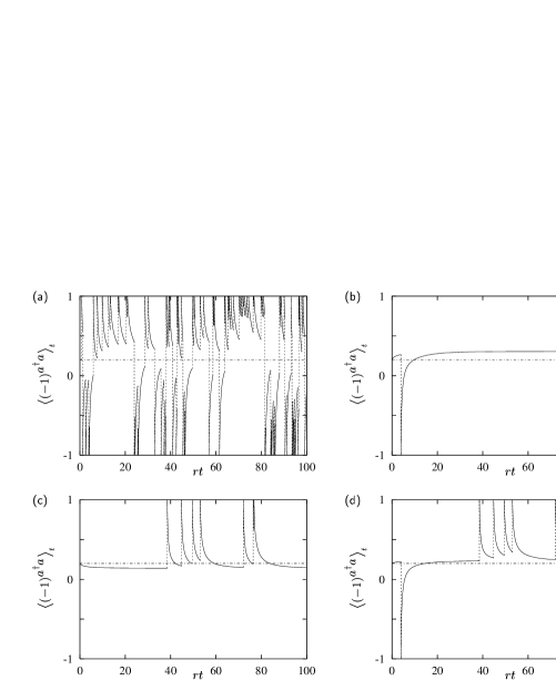
Figure 6: Different, but equally consistent, statistical predictions about the same physical system: Parity expectation value when parity measurements are performed on an unpumped resonator; see text

Figure 7: Different, but equally consistent, statistical predictions about the same physical system: Photon number expectation value when parity measurements are performed on an unpumped resonator; see text

Why, then, do we show Figs. 6(a) and 7(a) at all? Because one might think that they report the “true state of affairs” so that

$$\textrm{all atoms, }rt=60\,:\quad\bigl{\langle}(-1)^{\mbox{\footnotesize$a^{\dagger}a$}}\bigr{\rangle}=0.4818\;,\quad\bigl{\langle}a^{\dagger}a\bigr{\rangle}=1.189$$ (190)

would be the “true expectation values” of $(-1)^{\mbox{\footnotesize$a^{\dagger}a$}}$ and $a^{\dagger}a$ at $t=60/r$. And then one would conclude that the accounts given by Bob, Chuck, and Doris are wrong in some sense. In fact, all three give correct, though differing accounts, and the various predictions for $t=60/r$ in (186), (188), and (189) are all statistically correct. For, if you repeat the experiment very often you’ll find that Bob’s expectation values are confirmed by the data, and so are Chuck’s, and so are Doris’s.

But, of course, when extracting $\bigl{\langle}a^{\dagger}a\bigr{\rangle}_{t=60/r}$, say, from the data of the very many runs, you must take different subensembles for checking Bob’s predictions, or Chuck’s, or Doris’s. Bob’s prediction (186) refers to the subensemble characterized by a single click at $rt=3.88$ and no other click between $rt=0$ and $rt=60$, but any number of clicks. Likewise, Chuck’s prediction (188) is about the subensemble that has clicks at $rt$=38.51, 44.80, 49.52, and 53.07, no other clicks and any number of clicks. And Doris’s subensemble is specified by having this one click, these four clicks, and no other clicks of either kind. By contrast, no experimentally identifiable ensemble corresponds to Figs. 6(a) and 7(a); they represent sheer imagination, not phenomenological reality.

In summary, although it is the same physical object (the privileged mode of the resonator) that Bob, Chuck, and Doris make predictions about, they regard it as a representative of different ensembles, which are respectively characterized by the information taken into account. This illustrates the basic fact that a statistical operator is just an encoding of what we know about the system. Depending on the question we are asking, we may even have to ignore some of the information deliberately. The appropriate $\varrho_{t}$ is the one that pays due attention to the pertinent conditions under which we wish to make statistical predictions. Different conditions simply require different statistical operators. That there are several $\varrho_{t}$’s for the same physical object is then not bewildering, but rather expected.

The ensembles that Bob, Chuck, and Doris make statements about need not be, and usually are not, real ensembles created by many repeated runs of the experiment (or, since the system is ergodic DMEref:BESW94 ; DMEref:KueMaa01 , perhaps a single run of very long duration). Rather, they are Gibbs ensembles in the standard meaning of statistical mechanics: imagined ensembles characterized by the respective constraints and consistent weights. The constraints are duly taken into account by the nonlinear master equation (179).

We should also mention that Bob’s $\varrho_{t}$ is consistent with Chuck’s and Doris’s by construction. If we didn’t know how they arrive at their respective statistical operators we might wonder how we could verify that the three $\varrho_{t}$’s do not contradict each other. Consult DMEref:Mermin01a ; DMEref:Mermin01b if you find the question interesting.

Homework Assignments

1. Show that

   $$\sum_{m=0}^{\infty}y^{m}\check{\varrho}_{m}^{(0)}=\frac{1+\nu}{1+\nu+\nu y}\left(1+\frac{y}{1+\nu+\nu y}\right)^{\mbox{\footnotesize$a^{\dagger}a$}}$$ (191)

   is the $\nu>0$ generalization of (64), then use this and (60) to find the $\nu>0$ version of (163).

2. State the $\nu>0$ version of (164) and solve the equations for $n=0,1,2$.

3. Take the Scully–Lamb limit of (164), that is: $T\to 0$ after putting $p=rT$, and find the steady state values of all $\bar{\alpha}_{n}^{(0)}$’s.

4. Evaluate $\displaystyle\bar{\varrho}^{\mathrm{(ss)}}=\sum_{n=0}^{\infty}\bar{\alpha}_{n}^{(0)}\varrho_{n}^{(0)}$ for these $\bar{\alpha}_{n}^{(0)}$’s. You should obtain

   $$\bar{\varrho}^{\mathrm{(ss)}}=\frac{1}{\nu+1}\left(\frac{\nu}{\nu+1}\right)^{\mbox{\footnotesize$a^{\dagger}a$}}\mathrm{L}_{\mbox{\footnotesize$a^{\dagger}a$}}^{(0)}\left(-\frac{r}{\nu A}\right)\,\mathrm{e}^{\mbox{\footnotesize$-r/A$}}\;.$$ (192)

   In which sense is this yet another generating function for the $\varrho_{n}^{(0)}$’s? What do you get for $\nu\to 0$?

5. Verify (173) for $\mathcal{B}$ of (4.2).

6. Show that

   $$\mathcal{M}f(a^{\dagger}a)=\left[\sin\left(\phi\sqrt{a^{\dagger}a}\,\right)\right]^{2}f(a^{\dagger}a-1)-\left[\sin\left(\phi\sqrt{a^{\dagger}a+1}\,\right)\right]^{2}f(a^{\dagger}a)$$ (193)

   for $\mathcal{M}$ of (167), then combine this with (41) to find the steady state of the Scully–Lamb equation (151). You should get

   $$\varrho^{\mathrm{(ss)}}=N\prod_{n=1}^{\mbox{\footnotesize$a^{\dagger}a$}}\left[\frac{\nu}{\nu+1}+\frac{r/A}{\nu+1}\left(\frac{\sin\left(\phi\sqrt{n}\,\right)}{\sqrt{n}}\right)^{2}\right]$$ (194)

   as the steady state of the one-atom maser. What is the physical significance of the normalization factor $N$? How do you determine it?

7. Differentiate $\varrho_{t}$ of (181) to verify that it solves (179).

8. In addition to Bob, Chuck, and Doris, there is also Alice who pays attention to all detector clicks but doesn’t care which detector fires. Which version of (179) does she employ, and how does she go about state reduction?

9. (a) Since you found Sect. 4.3 very puzzling, read it again.
   (b) If you are still puzzled, repeat (a), else proceed with (c).
   (c) Convince your favorite skeptical colleague that there can be different, but equally consistent, statistical operators for the same object.

5 Fifth Lecture: Statistics of Detected Atoms

A one-atom maser is operated under steady-state conditions. What is the probability to detect a atom between $t$ and $t+\mathrm{d}t$? It is

$$r\mathrm{d}t\,\eta_{\raisebox{-1.8pt}{\parbox[b]{8.00003pt}{\begin{picture}(10.0,8.0)(0.0,-1.8)\put(0.0,-1.8){\put(1.0,2.0){\line(1,0){8.0}}\put(1.0,6.0){\line(1,0){8.0}}\put(5.0,2.0){\circle*{2.5}}}\end{picture}}}}\,\mathrm{Tr}\left\{\mathcal{A}\varrho^{\mathrm{(ss)}}\right\}\;,$$ (195)

the product of the probability $r\mathrm{d}t$ of having an atom in this time interval ($r>0$ is taken for granted from here on) and the probability $\eta_{\raisebox{-1.8pt}{\parbox[b]{8.00003pt}{\begin{picture}(10.0,8.0)(0.0,-1.8)\put(0.0,-1.8){\put(1.0,2.0){\line(1,0){8.0}}\put(1.0,6.0){\line(1,0){8.0}}\put(5.0,2.0){\circle*{2.5}}}\end{picture}}}}\,\mathrm{Tr}\left\{\mathcal{A}\varrho^{\mathrm{(ss)}}\right\}$ that the detector clicks if there is an atom. Similarly,

$$r\mathrm{d}t\,\eta_{\raisebox{-1.8pt}{\parbox[b]{8.00003pt}{\begin{picture}(10.0,8.0)(0.0,-1.8)\put(0.0,-1.8){\put(1.0,2.0){\line(1,0){8.0}}\put(1.0,6.0){\line(1,0){8.0}}\put(5.0,6.0){\circle*{2.0}}}\end{picture}}}}\,\mathrm{Tr}\left\{\mathcal{B}\varrho^{\mathrm{(ss)}}\right\}$$ (196)

is the probability for a click between $t$ and $t+\mathrm{d}t$. What multiplies $r\mathrm{d}t$ here are the traces of the first and the second term of (171), respectively. The third term gave us the no-click probability (172).

The a priori probabilities (195) and (196) make no reference to other detection events. But the detector clicks are not statistically independent. For the example of the parity measurements of Sect. 4.3, you can see this very clearly in Fig. 6(d), where the even-parity clicks and the odd-parity clicks come in bunches. This bunching is easily understood: a click is accompanied by the state reduction (187) so that $\varrho_{t}$ is an even-parity state immediately after a click and, therefore, the next atom is much more likely to encounter even parity than odd parity. The detection of the first atom conditions the probabilities for the second atom, and for all subsequent ones as well.

5.1 Correlation Functions

Perhaps the simplest question one can ask in this context is: Given that a atom was detected at $t=0$, what is now the probability to detect a atom between $t$ and $t+\mathrm{d}t$? Since detection events that occur earlier than $t$ are not relevant here, we must use (179) with $\eta_{\raisebox{-1.8pt}{\parbox[b]{8.00003pt}{\begin{picture}(10.0,8.0)(0.0,-1.8)\put(0.0,-1.8){\put(1.0,2.0){\line(1,0){8.0}}\put(1.0,6.0){\line(1,0){8.0}}\put(5.0,2.0){\circle*{2.5}}}\end{picture}}}}=\eta_{\raisebox{-1.8pt}{\parbox[b]{8.00003pt}{\begin{picture}(10.0,8.0)(0.0,-1.8)\put(0.0,-1.8){\put(1.0,2.0){\line(1,0){8.0}}\put(1.0,6.0){\line(1,0){8.0}}\put(5.0,6.0){\circle*{2.0}}}\end{picture}}}}=0$ to propagate $\varrho_{t=0}$ to $\varrho_{t}$,

$$\varrho_{t}=\,\mathrm{e}^{\mbox{\footnotesize$\mathcal{L}_{0}t$}}\varrho_{t=0}$$ (197)

where

$$\mathcal{L}_{0}=\mathcal{L}_{\eta}\Big{|}_{\eta_{\raisebox{-1.8pt}{\parbox[b]{5.0pt}{\begin{picture}(10.0,8.0)(0.0,-1.8)\put(0.0,-1.8){\put(1.0,2.0){\line(1,0){8.0}}\put(1.0,6.0){\line(1,0){8.0}}\put(5.0,1.3){\makebox(0.0,0.0)[]{{\Large$\cdot$}}}}\end{picture}}}}=\eta_{\raisebox{-1.8pt}{\parbox[b]{5.0pt}{\begin{picture}(10.0,8.0)(0.0,-1.8)\put(0.0,-1.8){\put(1.0,2.0){\line(1,0){8.0}}\put(1.0,6.0){\line(1,0){8.0}}\put(5.0,5.3){\makebox(0.0,0.0)[]{{\Large$\cdot$}}}}\end{picture}}}}=0}=\mathcal{L}+r(\mathcal{A}+\mathcal{B}-1)$$ (198)

is the Liouville operator of the Scully–Lamb equation that determines the steady state,

$$\mathcal{L}_{0}\varrho^{\mathrm{(ss)}}=0\;,\qquad\lim_{t\to\infty}\,\mathrm{e}^{\mbox{\footnotesize$\mathcal{L}_{0}t$}}\varrho_{t=0}=\varrho^{\mathrm{(ss)}}\;.$$ (199)

The denominator of (181) equals unity here because $\mathcal{L}_{0}$ conserves the trace,

$$\,\mathrm{Tr}\left\{\,\mathrm{e}^{\mbox{\footnotesize$\mathcal{L}_{0}t$}}\varrho_{t=0}\right\}=\,\mathrm{Tr}\left\{\varrho_{t=0}\right\}=1\;.$$ (200)

With

$$\varrho_{t=0}=\frac{\mathcal{A}\varrho^{\mathrm{(ss)}}}{\,\mathrm{Tr}\left\{\mathcal{A}\varrho^{\mathrm{(ss)}}\right\}}$$ (201)

accounting for the initial click at $t=0$ (which, under steady-state conditions, is really any instant), the probability for a click at $t\cdots t+\mathrm{d}t$ is then

$$r\mathrm{d}t\,\eta_{\raisebox{-1.8pt}{\parbox[b]{8.00003pt}{\begin{picture}(10.0,8.0)(0.0,-1.8)\put(0.0,-1.8){\put(1.0,2.0){\line(1,0){8.0}}\put(1.0,6.0){\line(1,0){8.0}}\put(5.0,6.0){\circle*{2.0}}}\end{picture}}}}\,\mathrm{Tr}\left\{\mathcal{B}\,\mathrm{e}^{\mbox{\footnotesize$\mathcal{L}_{0}t$}}\varrho_{t=0}\right\}=r\mathrm{d}t\,\frac{\,\mathrm{Tr}\left\{\mathcal{B}\,\mathrm{e}^{\mbox{\footnotesize$\mathcal{L}_{0}t$}}\mathcal{A}\varrho^{\mathrm{(ss)}}\right\}}{\,\mathrm{Tr}\left\{\mathcal{A}\varrho^{\mathrm{(ss)}}\right\}}\;.$$ (202)

If $t$ is very late, the memory of the initial state gets lost and (202) becomes equal to the a priori probability (196). The ratio of the two probabilities,

$$G_{\raisebox{-1.8pt}{\parbox[b]{8.00003pt}{\begin{picture}(10.0,8.0)(0.0,-1.8)\put(0.0,-1.8){\put(1.0,2.0){\line(1,0){8.0}}\put(1.0,6.0){\line(1,0){8.0}}\put(5.0,2.0){\circle*{2.5}}}\end{picture}}}\raisebox{-1.8pt}{\parbox[b]{8.00003pt}{\begin{picture}(10.0,8.0)(0.0,-1.8)\put(0.0,-1.8){\put(1.0,2.0){\line(1,0){8.0}}\put(1.0,6.0){\line(1,0){8.0}}\put(5.0,6.0){\circle*{2.0}}}\end{picture}}}}(t)=\frac{\,\mathrm{Tr}\left\{\mathcal{B}\,\mathrm{e}^{\mbox{\footnotesize$\mathcal{L}_{0}t$}}\mathcal{A}\varrho^{\mathrm{(ss)}}\right\}}{\,\mathrm{Tr}\left\{\mathcal{B}\varrho^{\mathrm{(ss)}}\right\}\,\mathrm{Tr}\left\{\mathcal{A}\varrho^{\mathrm{(ss)}}\right\}}\;,$$ (203)

is the correlation function for clicks after clicks. There are no correlations if ${G_{\raisebox{-1.8pt}{\parbox[b]{8.00003pt}{\begin{picture}(10.0,8.0)(0.0,-1.8)\put(0.0,-1.8){\put(1.0,2.0){\line(1,0){8.0}}\put(1.0,6.0){\line(1,0){8.0}}\put(5.0,2.0){\circle*{2.5}}}\end{picture}}}\raisebox{-1.8pt}{\parbox[b]{8.00003pt}{\begin{picture}(10.0,8.0)(0.0,-1.8)\put(0.0,-1.8){\put(1.0,2.0){\line(1,0){8.0}}\put(1.0,6.0){\line(1,0){8.0}}\put(5.0,6.0){\circle*{2.0}}}\end{picture}}}}=1}$, positive correlations if ${G_{\raisebox{-1.8pt}{\parbox[b]{8.00003pt}{\begin{picture}(10.0,8.0)(0.0,-1.8)\put(0.0,-1.8){\put(1.0,2.0){\line(1,0){8.0}}\put(1.0,6.0){\line(1,0){8.0}}\put(5.0,2.0){\circle*{2.5}}}\end{picture}}}\raisebox{-1.8pt}{\parbox[b]{8.00003pt}{\begin{picture}(10.0,8.0)(0.0,-1.8)\put(0.0,-1.8){\put(1.0,2.0){\line(1,0){8.0}}\put(1.0,6.0){\line(1,0){8.0}}\put(5.0,6.0){\circle*{2.0}}}\end{picture}}}}>1}$, negative correlations if ${G_{\raisebox{-1.8pt}{\parbox[b]{8.00003pt}{\begin{picture}(10.0,8.0)(0.0,-1.8)\put(0.0,-1.8){\put(1.0,2.0){\line(1,0){8.0}}\put(1.0,6.0){\line(1,0){8.0}}\put(5.0,2.0){\circle*{2.5}}}\end{picture}}}\raisebox{-1.8pt}{\parbox[b]{8.00003pt}{\begin{picture}(10.0,8.0)(0.0,-1.8)\put(0.0,-1.8){\put(1.0,2.0){\line(1,0){8.0}}\put(1.0,6.0){\line(1,0){8.0}}\put(5.0,6.0){\circle*{2.0}}}\end{picture}}}}<1}$. The bunching of Fig. 6(d) shows strong negative correlations (odd after even) at short times.

Likewise, if we ask about clicks after clicks, we get

$$G_{\raisebox{-1.8pt}{\parbox[b]{8.00003pt}{\begin{picture}(10.0,8.0)(0.0,-1.8)\put(0.0,-1.8){\put(1.0,2.0){\line(1,0){8.0}}\put(1.0,6.0){\line(1,0){8.0}}\put(5.0,6.0){\circle*{2.0}}}\end{picture}}}\raisebox{-1.8pt}{\parbox[b]{8.00003pt}{\begin{picture}(10.0,8.0)(0.0,-1.8)\put(0.0,-1.8){\put(1.0,2.0){\line(1,0){8.0}}\put(1.0,6.0){\line(1,0){8.0}}\put(5.0,2.0){\circle*{2.5}}}\end{picture}}}}(t)=\frac{\,\mathrm{Tr}\left\{\mathcal{A}\,\mathrm{e}^{\mbox{\footnotesize$\mathcal{L}_{0}t$}}\mathcal{B}\varrho^{\mathrm{(ss)}}\right\}}{\,\mathrm{Tr}\left\{\mathcal{A}\varrho^{\mathrm{(ss)}}\right\}\,\mathrm{Tr}\left\{\mathcal{B}\varrho^{\mathrm{(ss)}}\right\}}\;,$$ (204)

and we have

$$G_{\raisebox{-1.8pt}{\parbox[b]{8.00003pt}{\begin{picture}(10.0,8.0)(0.0,-1.8)\put(0.0,-1.8){\put(1.0,2.0){\line(1,0){8.0}}\put(1.0,6.0){\line(1,0){8.0}}\put(5.0,2.0){\circle*{2.5}}}\end{picture}}}\raisebox{-1.8pt}{\parbox[b]{8.00003pt}{\begin{picture}(10.0,8.0)(0.0,-1.8)\put(0.0,-1.8){\put(1.0,2.0){\line(1,0){8.0}}\put(1.0,6.0){\line(1,0){8.0}}\put(5.0,2.0){\circle*{2.5}}}\end{picture}}}}(t)=\frac{\,\mathrm{Tr}\left\{\mathcal{A}\,\mathrm{e}^{\mbox{\footnotesize$\mathcal{L}_{0}t$}}\mathcal{A}\varrho^{\mathrm{(ss)}}\right\}}{\left[\,\mathrm{Tr}\left\{\mathcal{A}\varrho^{\mathrm{(ss)}}\right\}\right]^{2}}\;,\qquad G_{\raisebox{-1.8pt}{\parbox[b]{8.00003pt}{\begin{picture}(10.0,8.0)(0.0,-1.8)\put(0.0,-1.8){\put(1.0,2.0){\line(1,0){8.0}}\put(1.0,6.0){\line(1,0){8.0}}\put(5.0,6.0){\circle*{2.0}}}\end{picture}}}\raisebox{-1.8pt}{\parbox[b]{8.00003pt}{\begin{picture}(10.0,8.0)(0.0,-1.8)\put(0.0,-1.8){\put(1.0,2.0){\line(1,0){8.0}}\put(1.0,6.0){\line(1,0){8.0}}\put(5.0,6.0){\circle*{2.0}}}\end{picture}}}}(t)=\frac{\,\mathrm{Tr}\left\{\mathcal{B}\,\mathrm{e}^{\mbox{\footnotesize$\mathcal{L}_{0}t$}}\mathcal{B}\varrho^{\mathrm{(ss)}}\right\}}{\left[\,\mathrm{Tr}\left\{\mathcal{B}\varrho^{\mathrm{(ss)}}\right\}\right]^{2}}\;,$$ (205)

for the correlation functions of clicks of the same kind. Note that the detection efficiencies $\eta_{\raisebox{-1.8pt}{\parbox[b]{8.00003pt}{\begin{picture}(10.0,8.0)(0.0,-1.8)\put(0.0,-1.8){\put(1.0,2.0){\line(1,0){8.0}}\put(1.0,6.0){\line(1,0){8.0}}\put(5.0,2.0){\circle*{2.5}}}\end{picture}}}},\eta_{\raisebox{-1.8pt}{\parbox[b]{8.00003pt}{\begin{picture}(10.0,8.0)(0.0,-1.8)\put(0.0,-1.8){\put(1.0,2.0){\line(1,0){8.0}}\put(1.0,6.0){\line(1,0){8.0}}\put(5.0,6.0){\circle*{2.0}}}\end{picture}}}}$ do not enter the correlation functions (203)–(205). This is a result of normalizing the conditional probabilities to the unconditional ones. But see homework assignment 26.

Figure 8: Correlation functions for parity measurements on an unpumped resonator. The solid $\frac{\qquad}{}$ line shows the even-even correlation function $G_{\raisebox{-1.8pt}{\parbox[b]{8.00003pt}{\begin{picture}(10.0,8.0)(0.0,-1.8)\put(0.0,-1.8){\put(1.0,2.0){\line(1,0){8.0}}\put(1.0,6.0){\line(1,0){8.0}}\put(5.0,2.0){\circle*{2.5}}}\end{picture}}}\raisebox{-1.8pt}{\parbox[b]{8.00003pt}{\begin{picture}(10.0,8.0)(0.0,-1.8)\put(0.0,-1.8){\put(1.0,2.0){\line(1,0){8.0}}\put(1.0,6.0){\line(1,0){8.0}}\put(5.0,2.0){\circle*{2.5}}}\end{picture}}}}(t)$, the dashed $---$ line the odd-odd correlation function $G_{\raisebox{-1.8pt}{\parbox[b]{8.00003pt}{\begin{picture}(10.0,8.0)(0.0,-1.8)\put(0.0,-1.8){\put(1.0,2.0){\line(1,0){8.0}}\put(1.0,6.0){\line(1,0){8.0}}\put(5.0,6.0){\circle*{2.0}}}\end{picture}}}\raisebox{-1.8pt}{\parbox[b]{8.00003pt}{\begin{picture}(10.0,8.0)(0.0,-1.8)\put(0.0,-1.8){\put(1.0,2.0){\line(1,0){8.0}}\put(1.0,6.0){\line(1,0){8.0}}\put(5.0,6.0){\circle*{2.0}}}\end{picture}}}}(t)$, and the dash-dotted $-\cdot-\cdot-$ line the cross correlations $G_{\raisebox{-1.8pt}{\parbox[b]{8.00003pt}{\begin{picture}(10.0,8.0)(0.0,-1.8)\put(0.0,-1.8){\put(1.0,2.0){\line(1,0){8.0}}\put(1.0,6.0){\line(1,0){8.0}}\put(5.0,2.0){\circle*{2.5}}}\end{picture}}}\raisebox{-1.8pt}{\parbox[b]{8.00003pt}{\begin{picture}(10.0,8.0)(0.0,-1.8)\put(0.0,-1.8){\put(1.0,2.0){\line(1,0){8.0}}\put(1.0,6.0){\line(1,0){8.0}}\put(5.0,6.0){\circle*{2.0}}}\end{picture}}}}(t)=G_{\raisebox{-1.8pt}{\parbox[b]{8.00003pt}{\begin{picture}(10.0,8.0)(0.0,-1.8)\put(0.0,-1.8){\put(1.0,2.0){\line(1,0){8.0}}\put(1.0,6.0){\line(1,0){8.0}}\put(5.0,6.0){\circle*{2.0}}}\end{picture}}}\raisebox{-1.8pt}{\parbox[b]{8.00003pt}{\begin{picture}(10.0,8.0)(0.0,-1.8)\put(0.0,-1.8){\put(1.0,2.0){\line(1,0){8.0}}\put(1.0,6.0){\line(1,0){8.0}}\put(5.0,2.0){\circle*{2.5}}}\end{picture}}}}(t)$. The plot is for $\nu=2$ in the expressions given in (210) and (5.1)

As an example we take once more the parity measurements of Figs. 6 and 7, for which $\mathcal{A},\mathcal{B}$ are given in (4.3) so that $\mathcal{L}_{0}=\mathcal{L}$. Then $\varrho^{\mathrm{(ss)}}$ is the thermal state of (44) and the a priori probabilities are

$$\,\mathrm{Tr}\left\{\mathcal{A}\varrho^{\mathrm{(ss)}}\right\} = {\displaystyle\frac{1}{2}}+{\displaystyle\frac{1}{2}}\bigl{\langle}(-1)^{\mbox{\footnotesize$a^{\dagger}a$}}\bigr{\rangle}^{\mathrm{(ss)}}=\frac{\nu+1}{2\nu+1}\;,$$

$$\,\mathrm{Tr}\left\{\mathcal{B}\varrho^{\mathrm{(ss)}}\right\} = {\displaystyle\frac{1}{2}}-{\displaystyle\frac{1}{2}}\bigl{\langle}(-1)^{\mbox{\footnotesize$a^{\dagger}a$}}\bigr{\rangle}^{\mathrm{(ss)}}=\frac{\nu}{2\nu+1}\;.$$ (206)

For $\nu=0$, there are no odd-parity clicks of the detector and, therefore, we’ll only consider the case of $\nu>0$. Since

$$\left.\begin{array}[]{l}\mathcal{A}\varrho^{\mathrm{(ss)}}\\[4.30554pt] \mathcal{B}\varrho^{\mathrm{(ss)}}\end{array}\right\}={\displaystyle\frac{1}{2}}\varrho^{\mathrm{(ss)}}\pm{\displaystyle\frac{1}{2}}\frac{1}{\nu+1}\left(-\frac{\nu}{\nu+1}\right)^{\mbox{\footnotesize$a^{\dagger}a$}}\;,$$ (207)

we have

$$\,\mathrm{e}^{\mbox{\footnotesize$\mathcal{L}_{0}t$}}(\mathcal{A}+\mathcal{B})\varrho^{\mathrm{(ss)}}=\varrho^{\mathrm{(ss)}}$$ (208)

and

$$\,\mathrm{e}^{\mbox{\footnotesize$\mathcal{L}_{0}t$}}(\mathcal{A}-\mathcal{B})\varrho^{\mathrm{(ss)}}=\frac{1}{2\nu+1}\lambda(t)\bigl{[}1-\lambda(t)\bigr{]}^{\mbox{\footnotesize$a^{\dagger}a$}}\;,$$ (209)

where $\lambda(t)$ is given in (55) with $\lambda(0)=(2\nu+1)/(\nu+1)$. The numerators of (203)–(205) are then easily evaluated and we obtain

$$G_{\raisebox{-1.8pt}{\parbox[b]{8.00003pt}{\begin{picture}(10.0,8.0)(0.0,-1.8)\put(0.0,-1.8){\put(1.0,2.0){\line(1,0){8.0}}\put(1.0,6.0){\line(1,0){8.0}}\put(5.0,2.0){\circle*{2.5}}}\end{picture}}}\raisebox{-1.8pt}{\parbox[b]{8.00003pt}{\begin{picture}(10.0,8.0)(0.0,-1.8)\put(0.0,-1.8){\put(1.0,2.0){\line(1,0){8.0}}\put(1.0,6.0){\line(1,0){8.0}}\put(5.0,6.0){\circle*{2.0}}}\end{picture}}}}(t)=G_{\raisebox{-1.8pt}{\parbox[b]{8.00003pt}{\begin{picture}(10.0,8.0)(0.0,-1.8)\put(0.0,-1.8){\put(1.0,2.0){\line(1,0){8.0}}\put(1.0,6.0){\line(1,0){8.0}}\put(5.0,6.0){\circle*{2.0}}}\end{picture}}}\raisebox{-1.8pt}{\parbox[b]{8.00003pt}{\begin{picture}(10.0,8.0)(0.0,-1.8)\put(0.0,-1.8){\put(1.0,2.0){\line(1,0){8.0}}\put(1.0,6.0){\line(1,0){8.0}}\put(5.0,2.0){\circle*{2.5}}}\end{picture}}}}(t)=1-\left[1+(2\nu+1)^{2}(\,\mathrm{e}^{\mbox{\footnotesize$At$}}-1)\right]^{-1}$$ (210)

and

$$G_{\raisebox{-1.8pt}{\parbox[b]{8.00003pt}{\begin{picture}(10.0,8.0)(0.0,-1.8)\put(0.0,-1.8){\put(1.0,2.0){\line(1,0){8.0}}\put(1.0,6.0){\line(1,0){8.0}}\put(5.0,2.0){\circle*{2.5}}}\end{picture}}}\raisebox{-1.8pt}{\parbox[b]{8.00003pt}{\begin{picture}(10.0,8.0)(0.0,-1.8)\put(0.0,-1.8){\put(1.0,2.0){\line(1,0){8.0}}\put(1.0,6.0){\line(1,0){8.0}}\put(5.0,2.0){\circle*{2.5}}}\end{picture}}}}(t) = 1+\frac{\nu}{\nu+1}\left[1+(2\nu+1)^{2}(\,\mathrm{e}^{\mbox{\footnotesize$At$}}-1)\right]^{-1}\;,$$

$$G_{\raisebox{-1.8pt}{\parbox[b]{8.00003pt}{\begin{picture}(10.0,8.0)(0.0,-1.8)\put(0.0,-1.8){\put(1.0,2.0){\line(1,0){8.0}}\put(1.0,6.0){\line(1,0){8.0}}\put(5.0,6.0){\circle*{2.0}}}\end{picture}}}\raisebox{-1.8pt}{\parbox[b]{8.00003pt}{\begin{picture}(10.0,8.0)(0.0,-1.8)\put(0.0,-1.8){\put(1.0,2.0){\line(1,0){8.0}}\put(1.0,6.0){\line(1,0){8.0}}\put(5.0,6.0){\circle*{2.0}}}\end{picture}}}}(t) = 1+\frac{\nu+1}{\nu}\left[1+(2\nu+1)^{2}(\,\mathrm{e}^{\mbox{\footnotesize$At$}}-1)\right]^{-1}\;.$$ (211)

The cross correlations of (210) vanish at $t=0$ (no even-parity click immediately after an odd-parity click and vice versa) and increase monotonically toward $1$. The two same-click correlation functions of (5.1) are always larger than $1$ and decrease monotonically from their $t=0$ values

$$G_{\raisebox{-1.8pt}{\parbox[b]{8.00003pt}{\begin{picture}(10.0,8.0)(0.0,-1.8)\put(0.0,-1.8){\put(1.0,2.0){\line(1,0){8.0}}\put(1.0,6.0){\line(1,0){8.0}}\put(5.0,2.0){\circle*{2.5}}}\end{picture}}}\raisebox{-1.8pt}{\parbox[b]{8.00003pt}{\begin{picture}(10.0,8.0)(0.0,-1.8)\put(0.0,-1.8){\put(1.0,2.0){\line(1,0){8.0}}\put(1.0,6.0){\line(1,0){8.0}}\put(5.0,2.0){\circle*{2.5}}}\end{picture}}}}(t=0)=\frac{2\nu+1}{\nu+1}\;,\qquad G_{\raisebox{-1.8pt}{\parbox[b]{8.00003pt}{\begin{picture}(10.0,8.0)(0.0,-1.8)\put(0.0,-1.8){\put(1.0,2.0){\line(1,0){8.0}}\put(1.0,6.0){\line(1,0){8.0}}\put(5.0,6.0){\circle*{2.0}}}\end{picture}}}\raisebox{-1.8pt}{\parbox[b]{8.00003pt}{\begin{picture}(10.0,8.0)(0.0,-1.8)\put(0.0,-1.8){\put(1.0,2.0){\line(1,0){8.0}}\put(1.0,6.0){\line(1,0){8.0}}\put(5.0,6.0){\circle*{2.0}}}\end{picture}}}}(t=0)=\frac{2\nu+1}{\nu}\;,$$ (212)

which exceed unity and so confirm the bunching observed in Fig. 6(d). For $\nu=2$, the parameter value of Figs. 6 and 7, the correlation functions are plotted in Fig. 8.

Data of actual measurements of correlation functions for atoms emerging from a real-life micromaser are reported in DMEref:ELBVWW98 , for example. Theoretical values for some related quantities, such as the mean number of successive detector clicks of the same kind, agree very well with the experimental findings.

5.2 Waiting Time Statistics

Here is a different question: A click happened at $t=0$, what is the probability that the next clicks occurs between $t$ and $t+\mathrm{d}t$? In marked contrast to the question asked before (197), we are now not interested in any later click, but in the next click, and this just says that there are no other clicks before $t$. Since we ignore deliberately all clicks at intermediate times, we have to use (179) with $\eta_{\raisebox{-1.8pt}{\parbox[b]{8.00003pt}{\begin{picture}(10.0,8.0)(0.0,-1.8)\put(0.0,-1.8){\put(1.0,2.0){\line(1,0){8.0}}\put(1.0,6.0){\line(1,0){8.0}}\put(5.0,6.0){\circle*{2.0}}}\end{picture}}}}=0$ in the click operator $\mathcal{C}$ of (174).

We introduce the following quantities:

$$\begin{array}[b]{rcl}r\mathrm{d}t\,p_{\raisebox{-1.8pt}{\parbox[b]{8.00003pt}{\begin{picture}(10.0,8.0)(0.0,-1.8)\put(0.0,-1.8){\put(1.0,2.0){\line(1,0){8.0}}\put(1.0,6.0){\line(1,0){8.0}}\put(5.0,2.0){\circle*{2.5}}}\end{picture}}}}(t)&=&\mbox{probability for a $\raisebox{-1.8pt}{\parbox[b]{10.0pt}{\begin{picture}(10.0,8.0)(0.0,-1.8)\put(0.0,-1.8){\put(1.0,2.0){\line(1,0){8.0}}\put(1.0,6.0){\line(1,0){8.0}}\put(5.0,2.0){\circle*{2.5}}}\end{picture}}}$ click at $t\cdots t+\mathrm{d}t$}\;,\\[4.30554pt] p_{\mathrm{no}\raisebox{-1.8pt}{\parbox[b]{8.00003pt}{\begin{picture}(10.0,8.0)(0.0,-1.8)\put(0.0,-1.8){\put(1.0,2.0){\line(1,0){8.0}}\put(1.0,6.0){\line(1,0){8.0}}\put(5.0,2.0){\circle*{2.5}}}\end{picture}}}}(t)&=&\mbox{probability for no $\raisebox{-1.8pt}{\parbox[b]{10.0pt}{\begin{picture}(10.0,8.0)(0.0,-1.8)\put(0.0,-1.8){\put(1.0,2.0){\line(1,0){8.0}}\put(1.0,6.0){\line(1,0){8.0}}\put(5.0,2.0){\circle*{2.5}}}\end{picture}}}$ click before $t$}\;,\\[4.30554pt] \mathrm{d}t\,P_{\mathrm{next}\raisebox{-1.8pt}{\parbox[b]{8.00003pt}{\begin{picture}(10.0,8.0)(0.0,-1.8)\put(0.0,-1.8){\put(1.0,2.0){\line(1,0){8.0}}\put(1.0,6.0){\line(1,0){8.0}}\put(5.0,2.0){\circle*{2.5}}}\end{picture}}}}(t)&=&\mbox{probability for the next $\raisebox{-1.8pt}{\parbox[b]{10.0pt}{\begin{picture}(10.0,8.0)(0.0,-1.8)\put(0.0,-1.8){\put(1.0,2.0){\line(1,0){8.0}}\put(1.0,6.0){\line(1,0){8.0}}\put(5.0,2.0){\circle*{2.5}}}\end{picture}}}$ click to happen at $t\cdots t+\mathrm{d}t$}\;.\end{array}$$ (213)

Since $1-r\mathrm{d}t\,p_{\raisebox{-1.8pt}{\parbox[b]{8.00003pt}{\begin{picture}(10.0,8.0)(0.0,-1.8)\put(0.0,-1.8){\put(1.0,2.0){\line(1,0){8.0}}\put(1.0,6.0){\line(1,0){8.0}}\put(5.0,2.0){\circle*{2.5}}}\end{picture}}}}(t)$ is then the probability that there is no click between $t$ and $t+\mathrm{d}t$, we have

$$p_{\mathrm{no}\raisebox{-1.8pt}{\parbox[b]{8.00003pt}{\begin{picture}(10.0,8.0)(0.0,-1.8)\put(0.0,-1.8){\put(1.0,2.0){\line(1,0){8.0}}\put(1.0,6.0){\line(1,0){8.0}}\put(5.0,2.0){\circle*{2.5}}}\end{picture}}}}(t+\mathrm{d}t)=p_{\mathrm{no}\raisebox{-1.8pt}{\parbox[b]{8.00003pt}{\begin{picture}(10.0,8.0)(0.0,-1.8)\put(0.0,-1.8){\put(1.0,2.0){\line(1,0){8.0}}\put(1.0,6.0){\line(1,0){8.0}}\put(5.0,2.0){\circle*{2.5}}}\end{picture}}}}(t)\bigl{[}1-r\mathrm{d}t\,p_{\raisebox{-1.8pt}{\parbox[b]{8.00003pt}{\begin{picture}(10.0,8.0)(0.0,-1.8)\put(0.0,-1.8){\put(1.0,2.0){\line(1,0){8.0}}\put(1.0,6.0){\line(1,0){8.0}}\put(5.0,2.0){\circle*{2.5}}}\end{picture}}}}(t)\bigr{]}$$

or $$p_{\raisebox{-1.8pt}{\parbox[b]{8.00003pt}{\begin{picture}(10.0,8.0)(0.0,-1.8)\put(0.0,-1.8){\put(1.0,2.0){\line(1,0){8.0}}\put(1.0,6.0){\line(1,0){8.0}}\put(5.0,2.0){\circle*{2.5}}}\end{picture}}}}(t)=-\frac{1}{r}\frac{\mathrm{d}}{\mathrm{d}t}\ln p_{\mathrm{no}\raisebox{-1.8pt}{\parbox[b]{8.00003pt}{\begin{picture}(10.0,8.0)(0.0,-1.8)\put(0.0,-1.8){\put(1.0,2.0){\line(1,0){8.0}}\put(1.0,6.0){\line(1,0){8.0}}\put(5.0,2.0){\circle*{2.5}}}\end{picture}}}}(t)\;,$$ (214)

and

$$p_{\mathrm{no}\raisebox{-1.8pt}{\parbox[b]{8.00003pt}{\begin{picture}(10.0,8.0)(0.0,-1.8)\put(0.0,-1.8){\put(1.0,2.0){\line(1,0){8.0}}\put(1.0,6.0){\line(1,0){8.0}}\put(5.0,2.0){\circle*{2.5}}}\end{picture}}}}(t+\mathrm{d}t)=p_{\mathrm{no}\raisebox{-1.8pt}{\parbox[b]{8.00003pt}{\begin{picture}(10.0,8.0)(0.0,-1.8)\put(0.0,-1.8){\put(1.0,2.0){\line(1,0){8.0}}\put(1.0,6.0){\line(1,0){8.0}}\put(5.0,2.0){\circle*{2.5}}}\end{picture}}}}(t)-\mathrm{d}t\,P_{\mathrm{next}\raisebox{-1.8pt}{\parbox[b]{8.00003pt}{\begin{picture}(10.0,8.0)(0.0,-1.8)\put(0.0,-1.8){\put(1.0,2.0){\line(1,0){8.0}}\put(1.0,6.0){\line(1,0){8.0}}\put(5.0,2.0){\circle*{2.5}}}\end{picture}}}}(t)$$

or $$P_{\mathrm{next}\raisebox{-1.8pt}{\parbox[b]{8.00003pt}{\begin{picture}(10.0,8.0)(0.0,-1.8)\put(0.0,-1.8){\put(1.0,2.0){\line(1,0){8.0}}\put(1.0,6.0){\line(1,0){8.0}}\put(5.0,2.0){\circle*{2.5}}}\end{picture}}}}(t)=-\frac{\mathrm{d}}{\mathrm{d}t}p_{\mathrm{no}\raisebox{-1.8pt}{\parbox[b]{8.00003pt}{\begin{picture}(10.0,8.0)(0.0,-1.8)\put(0.0,-1.8){\put(1.0,2.0){\line(1,0){8.0}}\put(1.0,6.0){\line(1,0){8.0}}\put(5.0,2.0){\circle*{2.5}}}\end{picture}}}}(t)$$ (215)

is another immediate consequence of the significance given to these quantities.

We know $p_{\raisebox{-1.8pt}{\parbox[b]{8.00003pt}{\begin{picture}(10.0,8.0)(0.0,-1.8)\put(0.0,-1.8){\put(1.0,2.0){\line(1,0){8.0}}\put(1.0,6.0){\line(1,0){8.0}}\put(5.0,2.0){\circle*{2.5}}}\end{picture}}}}(t)$ from (172) and (181),

$$p_{\raisebox{-1.8pt}{\parbox[b]{8.00003pt}{\begin{picture}(10.0,8.0)(0.0,-1.8)\put(0.0,-1.8){\put(1.0,2.0){\line(1,0){8.0}}\put(1.0,6.0){\line(1,0){8.0}}\put(5.0,2.0){\circle*{2.5}}}\end{picture}}}}(t)=\frac{\,\mathrm{Tr}\left\{\mathcal{C}\,\mathrm{e}^{\mbox{\footnotesize$\mathcal{L}_{\eta}t$}}\varrho_{t=0}\right\}}{\,\mathrm{Tr}\left\{\,\mathrm{e}^{\mbox{\footnotesize$\mathcal{L}_{\eta}t$}}\varrho_{t=0}\right\}}$$ (216)

where

$$\mathcal{C}=\eta_{\raisebox{-1.8pt}{\parbox[b]{8.00003pt}{\begin{picture}(10.0,8.0)(0.0,-1.8)\put(0.0,-1.8){\put(1.0,2.0){\line(1,0){8.0}}\put(1.0,6.0){\line(1,0){8.0}}\put(5.0,2.0){\circle*{2.5}}}\end{picture}}}}\mathcal{A}\qquad\mbox{and}\qquad\varrho_{t=0}=\frac{\mathcal{B}\varrho^{\mathrm{(ss)}}}{\,\mathrm{Tr}\left\{\mathcal{B}\varrho^{\mathrm{(ss)}}\right\}}$$ (217)

in the present context. As required by (5.2), the right-hand side of (216) must be a logarithmic derivative and, indeed, it is because the identity

$$\frac{\mathrm{d}}{\mathrm{d}t}\,\mathrm{Tr}\left\{\,\mathrm{e}^{\mbox{\footnotesize$\mathcal{L}_{\eta}t$}}\varrho_{t=0}\right\} = \,\mathrm{Tr}\left\{\mathcal{L}_{\eta}\,\mathrm{e}^{\mbox{\footnotesize$\mathcal{L}_{\eta}t$}}\varrho_{t=0}\right\}$$ (218)

$$= \,\mathrm{Tr}\left\{(\mathcal{L}_{0}-r\mathcal{C})\,\mathrm{e}^{\mbox{\footnotesize$\mathcal{L}_{\eta}t$}}\varrho_{t=0}\right\}$$

$$= -r\,\mathrm{Tr}\left\{\mathcal{C}\,\mathrm{e}^{\mbox{\footnotesize$\mathcal{L}_{\eta}t$}}\varrho_{t=0}\right\}\;,$$

which uses the trace-conserving property of $\mathcal{L}_{0}$, implies

$$p_{\raisebox{-1.8pt}{\parbox[b]{8.00003pt}{\begin{picture}(10.0,8.0)(0.0,-1.8)\put(0.0,-1.8){\put(1.0,2.0){\line(1,0){8.0}}\put(1.0,6.0){\line(1,0){8.0}}\put(5.0,2.0){\circle*{2.5}}}\end{picture}}}}(t)=-\frac{1}{r}\frac{\mathrm{d}}{\mathrm{d}t}\ln\,\mathrm{Tr}\left\{\,\mathrm{e}^{\mbox{\footnotesize$\mathcal{L}_{\eta}t$}}\varrho_{t=0}\right\}\;.$$ (219)

It follows that

$$p_{\mathrm{no}\raisebox{-1.8pt}{\parbox[b]{8.00003pt}{\begin{picture}(10.0,8.0)(0.0,-1.8)\put(0.0,-1.8){\put(1.0,2.0){\line(1,0){8.0}}\put(1.0,6.0){\line(1,0){8.0}}\put(5.0,2.0){\circle*{2.5}}}\end{picture}}}}(t)=\,\mathrm{Tr}\left\{\,\mathrm{e}^{\mbox{\footnotesize$\mathcal{L}_{\eta}t$}}\varrho_{t=0}\right\}\;,$$ (220)

and then (5.2), (218) give

$$P_{\mathrm{next}\raisebox{-1.8pt}{\parbox[b]{8.00003pt}{\begin{picture}(10.0,8.0)(0.0,-1.8)\put(0.0,-1.8){\put(1.0,2.0){\line(1,0){8.0}}\put(1.0,6.0){\line(1,0){8.0}}\put(5.0,2.0){\circle*{2.5}}}\end{picture}}}}(t)=r\,\mathrm{Tr}\left\{\mathcal{C}\,\mathrm{e}^{\mbox{\footnotesize$\mathcal{L}_{\eta}t$}}\varrho_{t=0}\right\}\;.$$ (221)

The “important physical significance” of the denominator in (179) that was left in limbo in Sect. 4.2 is finally revealed in (220): it is the probability that no atom is detected before $t$. Since an atom is surely detected if we just wait long enough, the limit

$$p_{\mathrm{no}\raisebox{-1.8pt}{\parbox[b]{8.00003pt}{\begin{picture}(10.0,8.0)(0.0,-1.8)\put(0.0,-1.8){\put(1.0,2.0){\line(1,0){8.0}}\put(1.0,6.0){\line(1,0){8.0}}\put(5.0,2.0){\circle*{2.5}}}\end{picture}}}}(t)\to 0\quad\mbox{as $t\to\infty$}$$ (222)

is a necessary property of $p_{\mathrm{no}\raisebox{-1.8pt}{\parbox[b]{8.00003pt}{\begin{picture}(10.0,8.0)(0.0,-1.8)\put(0.0,-1.8){\put(1.0,2.0){\line(1,0){8.0}}\put(1.0,6.0){\line(1,0){8.0}}\put(5.0,2.0){\circle*{2.5}}}\end{picture}}}}(t)$. As a consequence, all eigenvalues of $\mathcal{L}_{\eta}$ must have a negative real part.

Figure 9: Waiting time distributions for parity measurements on an unpumped resonator. The solid $\frac{\qquad}{}$ lines show $P_{\mathrm{next}}(t)/r$ for clicks after clicks (left) and clicks after clicks (right) as functions of $rt$. The dashed $---$ lines refer to clicks after clicks (left) and clicks after clicks (right). In these logarithmic plots, straight lines would correspond to the Poissonian statistics of uncorrelated clicks

Putting all things together we obtain

$$P_{\mathrm{next}\raisebox{-1.8pt}{\parbox[b]{8.00003pt}{\begin{picture}(10.0,8.0)(0.0,-1.8)\put(0.0,-1.8){\put(1.0,2.0){\line(1,0){8.0}}\put(1.0,6.0){\line(1,0){8.0}}\put(5.0,2.0){\circle*{2.5}}}\end{picture}}}}(t)=r\eta_{\raisebox{-1.8pt}{\parbox[b]{8.00003pt}{\begin{picture}(10.0,8.0)(0.0,-1.8)\put(0.0,-1.8){\put(1.0,2.0){\line(1,0){8.0}}\put(1.0,6.0){\line(1,0){8.0}}\put(5.0,2.0){\circle*{2.5}}}\end{picture}}}}\frac{\,\mathrm{Tr}\left\{\mathcal{A}\,\mathrm{e}^{\mbox{\footnotesize$(\mathcal{L}_{0}-r\eta_{\raisebox{-1.8pt}{\parbox[b]{5.0pt}{\begin{picture}(10.0,8.0)(0.0,-1.8)\put(0.0,-1.8){\put(1.0,2.0){\line(1,0){8.0}}\put(1.0,6.0){\line(1,0){8.0}}\put(5.0,1.3){\makebox(0.0,0.0)[]{{\Large$\cdot$}}}}\end{picture}}}}\mathcal{A})t$}}\mathcal{B}\varrho^{\mathrm{(ss)}}\right\}}{\,\mathrm{Tr}\left\{\mathcal{B}\varrho^{\mathrm{(ss)}}\right\}}$$ (223)

for the waiting time distribution for the next click after a click. Analogous expressions apply for the next click after a click, the next click after a click, and so forth. As a basic check of consistency we consider the situation in which $\mathcal{A}$ and $\mathcal{B}$ are just multiples of the identity,

$$\mathcal{A}\varrho_{t}=q\varrho_{t}\;,\qquad\mathcal{B}\varrho_{t}=(1-q)\varrho_{t}\qquad\mbox{with}\quad 0<q<1\;.$$ (224)

Then the detector clicks are not correlated at all and the waiting time distribution (223) should be Poissonian,

$$P_{\mathrm{next}\raisebox{-1.8pt}{\parbox[b]{8.00003pt}{\begin{picture}(10.0,8.0)(0.0,-1.8)\put(0.0,-1.8){\put(1.0,2.0){\line(1,0){8.0}}\put(1.0,6.0){\line(1,0){8.0}}\put(5.0,2.0){\circle*{2.5}}}\end{picture}}}}(t)=r\eta_{\raisebox{-1.8pt}{\parbox[b]{8.00003pt}{\begin{picture}(10.0,8.0)(0.0,-1.8)\put(0.0,-1.8){\put(1.0,2.0){\line(1,0){8.0}}\put(1.0,6.0){\line(1,0){8.0}}\put(5.0,2.0){\circle*{2.5}}}\end{picture}}}}q\,\mathrm{e}^{\mbox{\footnotesize$-r\eta_{\raisebox{-1.8pt}{\parbox[b]{8.00003pt}{\begin{picture}(10.0,8.0)(0.0,-1.8)\put(0.0,-1.8){\put(1.0,2.0){\line(1,0){8.0}}\put(1.0,6.0){\line(1,0){8.0}}\put(5.0,2.0){\circle*{2.5}}}\end{picture}}}}qt$}}\;,$$ (225)

and this is indeed what we get from (223) for (224).

Figure 9 shows the waiting time distributions to the parity measurements of Figs. 6–8. Other examples are presented in some figures of DMEref:BESW94 .

5.3 Counting Statistics

Yet another question is this: What is the probability $w_{n}(t)$ for detecting $n$ atoms in state during a period of duration $t$? We pay no attention to clicks and, therefore, have $\eta_{\raisebox{-1.8pt}{\parbox[b]{8.00003pt}{\begin{picture}(10.0,8.0)(0.0,-1.8)\put(0.0,-1.8){\put(1.0,2.0){\line(1,0){8.0}}\put(1.0,6.0){\line(1,0){8.0}}\put(5.0,6.0){\circle*{2.0}}}\end{picture}}}}=0$ in the nonlinear master equation (179) for the evolution between clicks.

Probability $w_{0}(t)$ is the no-click probability of Sect. 5.2,

$$w_{0}=\,\mathrm{Tr}\left\{\,\mathrm{e}^{\mbox{\footnotesize$\mathcal{L}_{\eta}t$}}\varrho^{\mathrm{(ss)}}\right\}\qquad\mbox{with}\qquad\mathcal{C}=\eta_{\raisebox{-1.8pt}{\parbox[b]{8.00003pt}{\begin{picture}(10.0,8.0)(0.0,-1.8)\put(0.0,-1.8){\put(1.0,2.0){\line(1,0){8.0}}\put(1.0,6.0){\line(1,0){8.0}}\put(5.0,2.0){\circle*{2.5}}}\end{picture}}}}\mathcal{A}\;,$$ (226)

where $\varrho_{t=0}=\varrho^{\mathrm{(ss)}}$ in (220) is appropriate now. The one-click probability $w_{1}(t)$ is given by

$$w_{1}(t)=r\int_{0}^{t}\mathrm{d}t^{\prime}\,\,\mathrm{Tr}\left\{\,\mathrm{e}^{\mbox{\footnotesize$\mathcal{L}_{\eta}(t-t^{\prime})$}}\varrho_{t=t^{\prime}+0}\right\}\,\mathrm{Tr}\left\{\mathcal{C}\varrho_{t=t^{\prime}-0}\right\}\,\mathrm{Tr}\left\{\,\mathrm{e}^{\mbox{\footnotesize$\mathcal{L}_{\eta}t^{\prime}$}}\varrho^{\mathrm{(ss)}}\right\}\;,$$ (227)

where the last factor is the probability $w_{0}(t^{\prime})$ for no click before $t^{\prime}$, the first factor is the probability for no click after $t^{\prime}$, and

$$r\mathrm{d}t^{\prime}\,\,\mathrm{Tr}\left\{\mathcal{C}\varrho_{t=t^{\prime}-0}\right\}$$ (228)

is the probability for a click at $t^{\prime}$. In accordance with (181) and (187), the statistical operators just before and after the click at $t^{\prime}$ are

$$\varrho_{t=t^{\prime}-0}=\frac{\,\mathrm{e}^{\mbox{\footnotesize$\mathcal{L}_{\eta}t^{\prime}$}}\varrho^{\mathrm{(ss)}}}{\,\mathrm{Tr}\left\{\,\mathrm{e}^{\mbox{\footnotesize$\mathcal{L}_{\eta}t^{\prime}$}}\varrho^{\mathrm{(ss)}}\right\}}$$ (229)

and

$$\varrho_{t=t^{\prime}+0}=\frac{\mathcal{A}\varrho_{t=t^{\prime}-0}}{\,\mathrm{Tr}\left\{\mathcal{A}\varrho_{t=t^{\prime}-0}\right\}}=\frac{\mathcal{C}\varrho_{t=t^{\prime}-0}}{\,\mathrm{Tr}\left\{\mathcal{C}\varrho_{t=t^{\prime}-0}\right\}}\;,$$ (230)

respectively, so that

$$\varrho_{t=t^{\prime}+0}\,\mathrm{Tr}\left\{\mathcal{C}\varrho_{t=t^{\prime}-0}\right\}\,\mathrm{Tr}\left\{\,\mathrm{e}^{\mbox{\footnotesize$\mathcal{L}_{\eta}t^{\prime}$}}\varrho^{\mathrm{(ss)}}\right\}=\mathcal{C}\,\mathrm{e}^{\mbox{\footnotesize$\mathcal{L}_{\eta}t^{\prime}$}}\varrho^{\mathrm{(ss)}}\;,$$ (231)

and a remarkable simplification happens, inasmuch as

$$w_{1}(t)=\int_{0}^{t}\mathrm{d}t^{\prime}\,\,\mathrm{Tr}\left\{\,\mathrm{e}^{\mbox{\footnotesize$\mathcal{L}_{\eta}(t-t^{\prime})$}}r\mathcal{C}\,\mathrm{e}^{\mbox{\footnotesize$\mathcal{L}_{\eta}t^{\prime}$}}\varrho^{\mathrm{(ss)}}\right\}$$ (232)

involves but a single trace as the equivalent replacement of the product of three traces with which we started in (227).

Upon writing (232) as a double integral

$$w_{1}(t)=\int_{0}^{\infty}\mathrm{d}t_{1}\,\int_{0}^{\infty}\mathrm{d}t_{0}\,\delta(t_{0}+t_{1}-t)\,\mathrm{Tr}\left\{\,\mathrm{e}^{\mbox{\footnotesize$\mathcal{L}_{\eta}t_{1}$}}r\mathcal{C}\,\mathrm{e}^{\mbox{\footnotesize$\mathcal{L}_{\eta}t_{0}$}}\varrho^{\mathrm{(ss)}}\right\}$$ (233)

it is reasonably obvious (and can be demonstrated by a simple induction) that

$$w_{n}(t) = \int_{0}^{\infty}\!\!\mathrm{d}t_{n}\,\int_{0}^{\infty}\!\!\mathrm{d}t_{n-1}\,\cdots\int_{0}^{\infty}\!\!\mathrm{d}t_{1}\,\int_{0}^{\infty}\!\!\mathrm{d}t_{0}\,\delta(t_{0}+t_{1}+\cdots+t_{n-1}+t_{n}-t)$$ (234)

$$\mbox{\quad}\times\,\mathrm{Tr}\left\{\,\mathrm{e}^{\mbox{\footnotesize$\mathcal{L}_{\eta}t_{n}$}}r\mathcal{C}\,\mathrm{e}^{\mbox{\footnotesize$\mathcal{L}_{\eta}t_{n-1}$}}r\mathcal{C}\cdots\,\mathrm{e}^{\mbox{\footnotesize$\mathcal{L}_{\eta}t_{1}$}}r\mathcal{C}\,\mathrm{e}^{\mbox{\footnotesize$\mathcal{L}_{\eta}t_{0}$}}\varrho^{\mathrm{(ss)}}\right\}$$

or

$$w_{n}(t)=\,\mathrm{Tr}\left\{\mathcal{W}_{n}(t)\varrho^{\mathrm{(ss)}}\right\}\;.$$ (235)

The operator $\mathcal{W}_{n}(t)$ thus introduced,

$$\mathcal{W}_{n}(t)=\int_{0}^{\infty}\!\!\mathrm{d}t_{n}\,\cdots\int_{0}^{\infty}\!\!\mathrm{d}t_{0}\,\delta(t_{0}+\cdots+t_{n}-t)\,\mathrm{e}^{\mbox{\footnotesize$\mathcal{L}_{\eta}t_{n}$}}r\mathcal{C}\,\mathrm{e}^{\mbox{\footnotesize$\mathcal{L}_{\eta}t_{n-1}$}}\cdots r\mathcal{C}\,\mathrm{e}^{\mbox{\footnotesize$\mathcal{L}_{\eta}t_{0}$}}\;,$$ (236)

obeys the recurrence relation

$$\mathcal{W}_{n}(t)=\int_{0}^{t}\mathrm{d}t^{\prime}\,\mathcal{W}_{0}(t-t^{\prime})\,r\mathcal{C}\,\mathcal{W}_{n-1}(t^{\prime})\qquad\mbox{for $n=1,2,3,\dots$}$$ (237)

that commences with

$$\mathcal{W}_{0}(t)=\,\mathrm{e}^{\mbox{\footnotesize$\mathcal{L}_{\eta}t$}}\;.$$ (238)

As always, we’ll find it convenient to use a generating function,

$$\mathcal{W}(x,t)=\sum_{n=0}^{\infty}x^{n}\mathcal{W}_{n}(t)\;.$$ (239)

The recurrence relation for the $\mathcal{W}_{n}(t)$’s then turns into an integral equation for $\mathcal{W}(x,t)$,

$$\mathcal{W}(x,t)=\mathcal{W}_{0}(t)+\int_{0}^{t}\mathrm{d}t^{\prime}\,\mathcal{W}_{0}(t-t^{\prime})\,xr\mathcal{C}\,\mathcal{W}(x,t^{\prime})\;.$$ (240)

The standard technique for handling such finite-range convolutions utilizes Laplace transforms because the familiar identity

$$\int_{0}^{\infty}\!\!\mathrm{d}t\,\,\mathrm{e}^{\mbox{\footnotesize$-\gamma t$}}\int_{0}^{t}\!\mathrm{d}t^{\prime}\,f(t-t^{\prime})g(t^{\prime})=\int_{0}^{\infty}\!\!\mathrm{d}t\,\,\mathrm{e}^{\mbox{\footnotesize$-\gamma t$}}f(t)\int_{0}^{\infty}\!\!\mathrm{d}t^{\prime}\,\,\mathrm{e}^{\mbox{\footnotesize$-\gamma t^{\prime}$}}g(t^{\prime})$$ (241)

leads to a factorization. With

$$\int_{0}^{\infty}\!\!\mathrm{d}t\,\,\mathrm{e}^{\mbox{\footnotesize$-\gamma t$}}\mathcal{W}_{0}(t)=\bigl{(}\gamma-\mathcal{L}_{\eta}\bigr{)}^{-1}$$ (242)

this gets us to

$$\int_{0}^{\infty}\!\!\mathrm{d}t\,\,\mathrm{e}^{\mbox{\footnotesize$-\gamma t$}}\mathcal{W}(x,t) = \bigl{[}1-\bigl{(}\gamma-\mathcal{L}_{\eta}\bigr{)}^{-1}xr\mathcal{C}\bigr{]}^{-1}\bigl{(}\gamma-\mathcal{L}_{\eta}\bigr{)}^{-1}$$ (243)

$$= \Bigl{(}\bigl{(}\gamma-\mathcal{L}_{\eta}\bigr{)}\bigl{[}1-\bigl{(}\gamma-\mathcal{L}_{\eta}\bigr{)}^{-1}xr\mathcal{C}\bigr{]}\Bigr{)}^{-1}$$

$$= \bigl{(}\gamma-\mathcal{L}_{\eta}-xr\mathcal{C}\bigr{)}^{-1}\;,$$

and the inverse Laplace transform is elementary,

$$\mathcal{W}(x,t)=\,\mathrm{e}^{\mbox{\footnotesize$(\mathcal{L}_{\eta}+xr\mathcal{C})t$}}\;.$$ (244)

As we noted at (222), all eigenvalues of $\mathcal{L}_{\eta}$ have negative real parts, and so the Laplace transform (242) of $\mathcal{W}_{0}(t)$ surely exists for $\gamma\geq 0$. The same remark applies to $\mathcal{W}(x,t)$ for $-(1-\eta_{\raisebox{-1.8pt}{\parbox[b]{8.00003pt}{\begin{picture}(10.0,8.0)(0.0,-1.8)\put(0.0,-1.8){\put(1.0,2.0){\line(1,0){8.0}}\put(1.0,6.0){\line(1,0){8.0}}\put(5.0,2.0){\circle*{2.5}}}\end{picture}}}})/\eta_{\raisebox{-1.8pt}{\parbox[b]{8.00003pt}{\begin{picture}(10.0,8.0)(0.0,-1.8)\put(0.0,-1.8){\put(1.0,2.0){\line(1,0){8.0}}\put(1.0,6.0){\line(1,0){8.0}}\put(5.0,2.0){\circle*{2.5}}}\end{picture}}}}<x<1$ because

$$\mathcal{L}_{\eta}+xr\mathcal{C}=\mathcal{L}_{0}-(1-x)r\mathcal{C}=\mathcal{L}_{0}-r(1-x)\eta_{\raisebox{-1.8pt}{\parbox[b]{8.00003pt}{\begin{picture}(10.0,8.0)(0.0,-1.8)\put(0.0,-1.8){\put(1.0,2.0){\line(1,0){8.0}}\put(1.0,6.0){\line(1,0){8.0}}\put(5.0,2.0){\circle*{2.5}}}\end{picture}}}}\mathcal{A}$$ (245)

is $\mathcal{L}_{\eta}$ with $\eta_{\raisebox{-1.8pt}{\parbox[b]{8.00003pt}{\begin{picture}(10.0,8.0)(0.0,-1.8)\put(0.0,-1.8){\put(1.0,2.0){\line(1,0){8.0}}\put(1.0,6.0){\line(1,0){8.0}}\put(5.0,2.0){\circle*{2.5}}}\end{picture}}}}$ replaced by $(1-x)\eta_{\raisebox{-1.8pt}{\parbox[b]{8.00003pt}{\begin{picture}(10.0,8.0)(0.0,-1.8)\put(0.0,-1.8){\put(1.0,2.0){\line(1,0){8.0}}\put(1.0,6.0){\line(1,0){8.0}}\put(5.0,2.0){\circle*{2.5}}}\end{picture}}}}$ so that $\mathcal{L}_{\eta}+xr\mathcal{C}$ is just another operator of the same kind as $\mathcal{L}_{\eta}$ if the “effective detection efficiency” $(1-x)\eta_{\raisebox{-1.8pt}{\parbox[b]{8.00003pt}{\begin{picture}(10.0,8.0)(0.0,-1.8)\put(0.0,-1.8){\put(1.0,2.0){\line(1,0){8.0}}\put(1.0,6.0){\line(1,0){8.0}}\put(5.0,2.0){\circle*{2.5}}}\end{picture}}}}$ is in the range $0\cdots 1$, which restricts $x$ to the range stated above.

After putting things together we obtain

$$\sum_{n=0}^{\infty}x^{n}w_{n}(t)=\,\mathrm{Tr}\left\{\,\mathrm{e}^{\mbox{\footnotesize$(\mathcal{L}_{\eta}+xr\mathcal{C})t$}}\varrho^{\mathrm{(ss)}}\right\}$$ (246)

as the generating function for the counting probabilities $w_{n}(t)$. In view of what we observed above about $\mathcal{L}_{\eta}+xr\mathcal{C}$, the right-hand side of (246) is equal to the no-click probability $w_{0}(t)$ for detection efficiency $(1-x)\eta_{\raisebox{-1.8pt}{\parbox[b]{8.00003pt}{\begin{picture}(10.0,8.0)(0.0,-1.8)\put(0.0,-1.8){\put(1.0,2.0){\line(1,0){8.0}}\put(1.0,6.0){\line(1,0){8.0}}\put(5.0,2.0){\circle*{2.5}}}\end{picture}}}}$. Accordingly, $w_{0}(t)$ determines all $w_{n}(t)$ through its dependence on $\eta_{\raisebox{-1.8pt}{\parbox[b]{8.00003pt}{\begin{picture}(10.0,8.0)(0.0,-1.8)\put(0.0,-1.8){\put(1.0,2.0){\line(1,0){8.0}}\put(1.0,6.0){\line(1,0){8.0}}\put(5.0,2.0){\circle*{2.5}}}\end{picture}}}}$. As an immediate consequence of this observation, we get a statement about the moments of the counting statistics,

$$\sum_{n=0}^{\infty}{n\choose k}w_{n}(t)=\frac{1}{k!}\left(\frac{\partial}{\partial x}\right)^{k}\sum_{n=0}^{\infty}x^{n}w_{n}(t)\Big{|}_{x=1}=\eta_{\raisebox{-1.8pt}{\parbox[b]{8.00003pt}{\begin{picture}(10.0,8.0)(0.0,-1.8)\put(0.0,-1.8){\put(1.0,2.0){\line(1,0){8.0}}\put(1.0,6.0){\line(1,0){8.0}}\put(5.0,2.0){\circle*{2.5}}}\end{picture}}}}^{k}\left[\eta_{\raisebox{-1.8pt}{\parbox[b]{8.00003pt}{\begin{picture}(10.0,8.0)(0.0,-1.8)\put(0.0,-1.8){\put(1.0,2.0){\line(1,0){8.0}}\put(1.0,6.0){\line(1,0){8.0}}\put(5.0,2.0){\circle*{2.5}}}\end{picture}}}}^{-k}w_{k}(t)\Big{|}_{\eta_{\raisebox{-1.8pt}{\parbox[b]{5.0pt}{\begin{picture}(10.0,8.0)(0.0,-1.8)\put(0.0,-1.8){\put(1.0,2.0){\line(1,0){8.0}}\put(1.0,6.0){\line(1,0){8.0}}\put(5.0,1.3){\makebox(0.0,0.0)[]{{\Large$\cdot$}}}}\end{picture}}}}\to 0}\right]\;.$$ (247)

For $k=0$, we check the normalization,

$$\sum_{n=0}^{\infty}w_{n}(t)=\,\mathrm{Tr}\left\{\,\mathrm{e}^{\mbox{\footnotesize$\mathcal{L}_{0}t$}}\varrho^{\mathrm{(ss)}}\right\}=1\;;$$ (248)

for $k=1$, we get the average number of clicks,

$$\sum_{n=0}^{\infty}nw_{n}(t) = \int_{0}^{t}\mathrm{d}t^{\prime}\,\,\mathrm{Tr}\left\{\,\mathrm{e}^{\mbox{\footnotesize$\mathcal{L}_{0}(t-t^{\prime})$}}r\eta_{\raisebox{-1.8pt}{\parbox[b]{8.00003pt}{\begin{picture}(10.0,8.0)(0.0,-1.8)\put(0.0,-1.8){\put(1.0,2.0){\line(1,0){8.0}}\put(1.0,6.0){\line(1,0){8.0}}\put(5.0,2.0){\circle*{2.5}}}\end{picture}}}}\mathcal{A}\,\mathrm{e}^{\mbox{\footnotesize$\mathcal{L}_{0}t^{\prime}$}}\varrho^{\mathrm{(ss)}}\right\}$$ (249)

$$= \eta_{\raisebox{-1.8pt}{\parbox[b]{8.00003pt}{\begin{picture}(10.0,8.0)(0.0,-1.8)\put(0.0,-1.8){\put(1.0,2.0){\line(1,0){8.0}}\put(1.0,6.0){\line(1,0){8.0}}\put(5.0,2.0){\circle*{2.5}}}\end{picture}}}}rt\,\mathrm{Tr}\left\{\mathcal{A}\varrho^{\mathrm{(ss)}}\right\}\;,$$

which can be understood as a statement about the ergodicity of the process DMEref:BESW94 ; and for $k=2$, we learn something about the variance of the counting statistics,

$$\sum_{n=0}^{\infty}n(n-1)w_{n}(t)$$

$$\qquad=2\int_{0}^{t}\mathrm{d}t^{\prime}\,\int_{0}^{t^{\prime}}\mathrm{d}t^{\prime\prime}\,\,\mathrm{Tr}\left\{\,\mathrm{e}^{\mbox{\footnotesize$\mathcal{L}_{0}(t-t^{\prime})$}}r\eta_{\raisebox{-1.8pt}{\parbox[b]{8.00003pt}{\begin{picture}(10.0,8.0)(0.0,-1.8)\put(0.0,-1.8){\put(1.0,2.0){\line(1,0){8.0}}\put(1.0,6.0){\line(1,0){8.0}}\put(5.0,2.0){\circle*{2.5}}}\end{picture}}}}\mathcal{A}\,\mathrm{e}^{\mbox{\footnotesize$\mathcal{L}_{0}(t^{\prime}-t^{\prime\prime})$}}r\eta_{\raisebox{-1.8pt}{\parbox[b]{8.00003pt}{\begin{picture}(10.0,8.0)(0.0,-1.8)\put(0.0,-1.8){\put(1.0,2.0){\line(1,0){8.0}}\put(1.0,6.0){\line(1,0){8.0}}\put(5.0,2.0){\circle*{2.5}}}\end{picture}}}}\mathcal{A}\,\mathrm{e}^{\mbox{\footnotesize$\mathcal{L}_{0}t^{\prime\prime}$}}\varrho^{\mathrm{(ss)}}\right\}$$

$$\qquad=(\eta_{\raisebox{-1.8pt}{\parbox[b]{8.00003pt}{\begin{picture}(10.0,8.0)(0.0,-1.8)\put(0.0,-1.8){\put(1.0,2.0){\line(1,0){8.0}}\put(1.0,6.0){\line(1,0){8.0}}\put(5.0,2.0){\circle*{2.5}}}\end{picture}}}}rt)^{2}\,\mathrm{Tr}\left\{\mathcal{A}E(\mathcal{L}_{0}t)\mathcal{A}\varrho^{\mathrm{(ss)}}\right\}\;,$$ (250)

with

$$E(y)=\frac{2}{y^{2}}\bigl{(}\,\mathrm{e}^{\mbox{\footnotesize$y$}}-1-y\bigr{)}\;.$$ (251)

In traces of integrals such as (249) and (5.3), the exponential on the left and on the right can be ignored because $\mathcal{L}_{0}$ is trace conserving and $\varrho^{\mathrm{(ss)}}$ is its right eigenvector to eigenvalue zero.

Here, too, we get Poissonian statistics for (224), namely

$$\sum_{n=0}^{\infty}x^{n}w_{n}(t)=\,\mathrm{e}^{\mbox{\footnotesize$-(1-x)r\eta_{\raisebox{-1.8pt}{\parbox[b]{5.0pt}{\begin{picture}(10.0,8.0)(0.0,-1.8)\put(0.0,-1.8){\put(1.0,2.0){\line(1,0){8.0}}\put(1.0,6.0){\line(1,0){8.0}}\put(5.0,1.3){\makebox(0.0,0.0)[]{{\Large$\cdot$}}}}\end{picture}}}}qt$}}\;,\qquad w_{n}(t)=\frac{(r\eta_{\raisebox{-1.8pt}{\parbox[b]{8.00003pt}{\begin{picture}(10.0,8.0)(0.0,-1.8)\put(0.0,-1.8){\put(1.0,2.0){\line(1,0){8.0}}\put(1.0,6.0){\line(1,0){8.0}}\put(5.0,2.0){\circle*{2.5}}}\end{picture}}}}qt)^{n}}{n!}\,\mathrm{e}^{\mbox{\footnotesize$-r\eta_{\raisebox{-1.8pt}{\parbox[b]{5.0pt}{\begin{picture}(10.0,8.0)(0.0,-1.8)\put(0.0,-1.8){\put(1.0,2.0){\line(1,0){8.0}}\put(1.0,6.0){\line(1,0){8.0}}\put(5.0,1.3){\makebox(0.0,0.0)[]{{\Large$\cdot$}}}}\end{picture}}}}qt$}}\;,$$ (252)

for which

$$\sum_{n=0}^{\infty}{n\choose k}w_{n}(t)=\frac{(r\eta_{\raisebox{-1.8pt}{\parbox[b]{8.00003pt}{\begin{picture}(10.0,8.0)(0.0,-1.8)\put(0.0,-1.8){\put(1.0,2.0){\line(1,0){8.0}}\put(1.0,6.0){\line(1,0){8.0}}\put(5.0,2.0){\circle*{2.5}}}\end{picture}}}}qt)^{k}}{k!}\;.$$ (253)

In particular, we note that

$$\sum_{n=0}^{\infty}n(n-1)w_{n}(t)=\left[\sum_{n=0}^{\infty}nw_{n}(t)\right]^{2}$$ (254)

holds for the Poissonian counting statistics (252).

A convenient, yet rough, measure for the deviation from Poissonian statistics is the so-called Fano–Mandel factor $Q(t)$,

$$Q=\frac{\displaystyle\sum_{n=0}^{\infty}n(n-1)w_{n}}{\displaystyle\sum_{n=0}^{\infty}nw_{n}}-\sum_{n=0}^{\infty}nw_{n}\;,$$ (255)

a normalized variance. The normalization is such that $Q=0$ for Poissonian counting statistics, as one verifies easily with (254). For ${-1\leq Q<0}$ one speaks of sub-Poissonian statistics, and of super-Poissonian statistics for $Q>0$.

Figure 10: Fano–Mandel factor for the counting statistics in parity measurements on an unpumped resonator. The solid $\frac{\qquad}{}$ line shows $Q_{\raisebox{-1.8pt}{\parbox[b]{8.00003pt}{\begin{picture}(10.0,8.0)(0.0,-1.8)\put(0.0,-1.8){\put(1.0,2.0){\line(1,0){8.0}}\put(1.0,6.0){\line(1,0){8.0}}\put(5.0,2.0){\circle*{2.5}}}\end{picture}}}}(t)$ of (258), the horizontal dashed $---$ line is the asymptotic value of (259)

For the count of clicks, (249) and (5.3) give

$$Q_{\raisebox{-1.8pt}{\parbox[b]{8.00003pt}{\begin{picture}(10.0,8.0)(0.0,-1.8)\put(0.0,-1.8){\put(1.0,2.0){\line(1,0){8.0}}\put(1.0,6.0){\line(1,0){8.0}}\put(5.0,2.0){\circle*{2.5}}}\end{picture}}}}(t)=\eta_{\raisebox{-1.8pt}{\parbox[b]{8.00003pt}{\begin{picture}(10.0,8.0)(0.0,-1.8)\put(0.0,-1.8){\put(1.0,2.0){\line(1,0){8.0}}\put(1.0,6.0){\line(1,0){8.0}}\put(5.0,2.0){\circle*{2.5}}}\end{picture}}}}rt\left[\frac{\,\mathrm{Tr}\left\{\mathcal{A}E(\mathcal{L}_{0}t)\mathcal{A}\varrho^{\mathrm{(ss)}}\right\}}{\,\mathrm{Tr}\left\{\mathcal{A}\varrho^{\mathrm{(ss)}}\right\}}-\,\mathrm{Tr}\left\{\mathcal{A}\varrho^{\mathrm{(ss)}}\right\}\right]\;.$$ (256)

We use the damping bases to get a tractable numerical expression,

$$Q_{\raisebox{-1.8pt}{\parbox[b]{8.00003pt}{\begin{picture}(10.0,8.0)(0.0,-1.8)\put(0.0,-1.8){\put(1.0,2.0){\line(1,0){8.0}}\put(1.0,6.0){\line(1,0){8.0}}\put(5.0,2.0){\circle*{2.5}}}\end{picture}}}}(t)=\eta_{\raisebox{-1.8pt}{\parbox[b]{8.00003pt}{\begin{picture}(10.0,8.0)(0.0,-1.8)\put(0.0,-1.8){\put(1.0,2.0){\line(1,0){8.0}}\put(1.0,6.0){\line(1,0){8.0}}\put(5.0,2.0){\circle*{2.5}}}\end{picture}}}}rt\sum_{n=0}^{\infty}\sum_{k=-\infty}^{\infty}\bigl{(}1-\delta_{n,0}\delta_{k,0}\bigr{)}\frac{\,\mathrm{Tr}\left\{\mathcal{A}\varrho_{n}^{(k)}\right\}E(\lambda_{n}^{(k)}t)\,\mathrm{Tr}\left\{\check{\varrho}_{n}^{(k)}\mathcal{A}\varrho_{0}^{(0)}\right\}}{\,\mathrm{Tr}\left\{\mathcal{A}\varrho_{0}^{(0)}\right\}}\;,$$ (257)

where the $n=0,k=0$ term is removed since $\varrho_{0}^{(0)}=\varrho^{\mathrm{(ss)}}$, $\check{\varrho}_{0}^{(0)}=1$, $\lambda_{0}^{(0)}=0$, and $E(y=0)=1$. For the parity measurements of Figs. 6–9, one can evaluate the sum and gets

$$Q_{\raisebox{-1.8pt}{\parbox[b]{8.00003pt}{\begin{picture}(10.0,8.0)(0.0,-1.8)\put(0.0,-1.8){\put(1.0,2.0){\line(1,0){8.0}}\put(1.0,6.0){\line(1,0){8.0}}\put(5.0,2.0){\circle*{2.5}}}\end{picture}}}}(t)=\frac{\eta_{\raisebox{-1.8pt}{\parbox[b]{8.00003pt}{\begin{picture}(10.0,8.0)(0.0,-1.8)\put(0.0,-1.8){\put(1.0,2.0){\line(1,0){8.0}}\put(1.0,6.0){\line(1,0){8.0}}\put(5.0,2.0){\circle*{2.5}}}\end{picture}}}}r}{(\nu+1)(2\nu+1)}\int_{0}^{t}\frac{\mathrm{d}t^{\prime}}{2At}\ln\Bigl{(}1+4\nu(\nu+1)\bigl{(}1-\,\mathrm{e}^{\mbox{\footnotesize$-At^{\prime}$}}\bigr{)}\Bigr{)}\;,$$ (258)

which is plotted in Fig. 10. For $At\ll 1$ and $At\gg 1$ the limiting forms

$$Q_{\raisebox{-1.8pt}{\parbox[b]{8.00003pt}{\begin{picture}(10.0,8.0)(0.0,-1.8)\put(0.0,-1.8){\put(1.0,2.0){\line(1,0){8.0}}\put(1.0,6.0){\line(1,0){8.0}}\put(5.0,2.0){\circle*{2.5}}}\end{picture}}}}(t)\simeq\left\{\begin{array}[]{l@{\mbox{\ for\ }}l}\displaystyle\frac{\nu}{2\nu+1}\eta_{\raisebox{-1.8pt}{\parbox[b]{8.00003pt}{\begin{picture}(10.0,8.0)(0.0,-1.8)\put(0.0,-1.8){\put(1.0,2.0){\line(1,0){8.0}}\put(1.0,6.0){\line(1,0){8.0}}\put(5.0,2.0){\circle*{2.5}}}\end{picture}}}}rt&At\ll 1\;,\\[8.61108pt] \displaystyle\frac{\ln(2\nu+1)}{(\nu+1)(2\nu+1)}\eta_{\raisebox{-1.8pt}{\parbox[b]{8.00003pt}{\begin{picture}(10.0,8.0)(0.0,-1.8)\put(0.0,-1.8){\put(1.0,2.0){\line(1,0){8.0}}\put(1.0,6.0){\line(1,0){8.0}}\put(5.0,2.0){\circle*{2.5}}}\end{picture}}}}r/A&At\gg 1\;,\end{array}\right.$$ (259)

obtain, as is confirmed by Fig. 10. Other examples of Fano–Mandel factors for counting statistics are presented in some figures of DMEref:BESW94 .

The pioneering measurement in 1990 of atom statistics in a real-life micromaser experiment is reported in DMEref:R+SK+W90 and linked to the photon counting statistics in DMEref:R+W90 . Measured Fano–Mandel factors from some later experiments can be found in DMEref:ELBVWW98 .

Homework Assignments

1. What is the correlation function for clicks of either kind, that is: without caring if it’s a click or a click?

2. The two cross-correlation functions are identical in the example of (5.1)–(212), see (210). Is this always the case?

3. Since the next click is bound to come sooner or later, consistency requires that $P_{\mathrm{next}}(t)$ is normalized to unit integral. Show that this is indeed so for $P_{\mathrm{next}}(t)$ of (221).

4. A click happens at $t=0$. What is the probability that the next click is a click?

5. Use the methods of Sect. 5.2 to find an expression for the average waiting time between successive clicks, between successive clicks.

6. Determine the short-time behavior of the various $P_{\mathrm{next}}$’s of Fig. 9 and compare with the plots.

7. Show that the exponential function $\,\mathrm{e}^{\mbox{\footnotesize$F$}}$ of an operator $F$ responds to variations $\delta F$ in accordance with

   $$\delta\,\mathrm{e}^{\mbox{\footnotesize$F$}}=\int_{0}^{1}\!\mathrm{d}\tau\,\,\mathrm{e}^{\mbox{\footnotesize$\tau F$}}\delta F\,\mathrm{e}^{\mbox{\footnotesize$(1-\tau)F$}}\;,$$ (260)

   which epitomizes all of perturbation theory.

8. Use (260) to extract $w_{1}(t)$ and $w_{2}(t)$ from (246). Compare with (234).

9. Consider the probability $w_{nm}(t)$ of detecting $n$ atoms in state and $m$ atoms in state during a period of duration $t$. Show that

   $$\sum_{n,m=0}^{\infty}x^{n}y^{m}w_{nm}(t)=\,\mathrm{Tr}\left\{\,\mathrm{e}^{\mbox{\footnotesize$(\mathcal{L}_{\eta}+xr\eta_{\raisebox{-1.8pt}{\parbox[b]{5.0pt}{\begin{picture}(10.0,8.0)(0.0,-1.8)\put(0.0,-1.8){\put(1.0,2.0){\line(1,0){8.0}}\put(1.0,6.0){\line(1,0){8.0}}\put(5.0,1.3){\makebox(0.0,0.0)[]{{\Large$\cdot$}}}}\end{picture}}}}\mathcal{A}+yr\eta_{\raisebox{-1.8pt}{\parbox[b]{5.0pt}{\begin{picture}(10.0,8.0)(0.0,-1.8)\put(0.0,-1.8){\put(1.0,2.0){\line(1,0){8.0}}\put(1.0,6.0){\line(1,0){8.0}}\put(5.0,5.3){\makebox(0.0,0.0)[]{{\Large$\cdot$}}}}\end{picture}}}}\mathcal{B})t$}}\varrho^{\mathrm{(ss)}}\right\}$$ (261)

   is the appropriate generalization of the generating function (246).

10. For $\mathcal{A}$ of (4.3), evaluate the $k=0$ traces in (257) and so confirm (258).

11. Find the leading correction to the approximation given in (259) for $At\gg 1$.

Appendix

Here are some facts about special functions that are useful for homework assignments 6 and 9. The expansion of (79) in powers of $\,\mathrm{e}^{\mbox{\footnotesize$-{\rm i}\omega t$}}\propto\bigl{[}\alpha(t)/\alpha^{*}(t)\bigr{]}^{\mbox{\footnotesize${\textstyle\frac{1}{2}}$}}$ is done with the aid of

$$\,\mathrm{e}^{\mbox{\footnotesize${\textstyle\frac{1}{2}}x(y-1/y)$}}=\sum_{k=-\infty}^{\infty}y^{k}\mathrm{J}_{k}(x)\;,$$ (262)

the most important generating function for Bessel functions of integer order,

$$\mathrm{J}_{k}(x)=(-1)^{k}\mathrm{J}_{-k}(x)={\rm i}^{|k|-k}\mathrm{J}_{|k|}(x)={\rm i}^{|k|-k}\sum_{m=0}^{\infty}\frac{(-1)^{m}}{m!\,(m+|k|)!}\left({\textstyle\frac{1}{2}}x\right)^{|k|+2m}\;.$$ (263)

They in turn act as a generating function for Laguerre polynomials,

$$\mathrm{J}_{|k|}\bigl{(}2\sqrt{xy}\,\bigr{)}=(xy)^{\mbox{\footnotesize${\textstyle\frac{1}{2}}|k|$}}\,\mathrm{e}^{\mbox{\footnotesize$-y$}}\sum_{n=0}^{\infty}\frac{y^{n}}{(n+|k|)!}\mathrm{L}_{n}^{(|k|)}(x)\;.$$ (264)

After a suitable Laplace transform this becomes

$$(1+y)^{-|k|-1}\,\mathrm{e}^{\mbox{\footnotesize$\frac{xy}{1+y}$}}=\sum_{n=0}^{\infty}(-y)^{n}\mathrm{L}_{n}^{(|k|)}(x)\;,$$ (265)

which is another useful generating function for the Laguerre polynomials

$$\mathrm{L}_{n}^{(|k|)}(x)=\sum_{m=0}^{n}{{n+|k|}\choose{m+|k|}}\frac{(-x)^{m}}{m!}\;.$$ (266)

The integral relations

$$\mathrm{L}_{n}^{(|k|)}(x)=\frac{1}{n!}\,\mathrm{e}^{\mbox{\footnotesize$x$}}x^{\mbox{\footnotesize$-{\textstyle\frac{1}{2}}|k|$}}\int_{0}^{\infty}\!\mathrm{d}y\,\,\mathrm{e}^{\mbox{\footnotesize$-y$}}y^{\mbox{\footnotesize$n+{\textstyle\frac{1}{2}}|k|$}}\mathrm{J}_{|k|}\bigl{(}2\sqrt{xy}\,\bigr{)}$$ (267)

and

$$\int_{0}^{\infty}\!\mathrm{d}y\,\,\mathrm{e}^{\mbox{\footnotesize$-y$}}\mathrm{J}_{|k|}\bigl{(}2\sqrt{uy}\,\bigr{)}\mathrm{J}_{|k|}\bigl{(}2\sqrt{vy}\,\bigr{)}=\,\mathrm{e}^{\mbox{\footnotesize$-(u+v)$}}\mathrm{I}_{k}\bigl{(}2\sqrt{uv}\,\bigr{)}$$ (268)

are worth knowing, where

$$\mathrm{I}_{k}(x)=\mathrm{I}_{-k}(x)={\rm i}^{-k}\mathrm{J}_{k}({\rm i}x)$$ (269)

are modified Bessel functions of integer order. As a preparation for homework assignment 6 you might want to derive first

$$\sum_{n=0}^{\infty}\frac{n!}{(n+|k|)!}x^{n}\mathrm{L}_{n}^{(|k|)}(y)\mathrm{L}_{n}^{(|k|)}(z)=\frac{(xyz)^{\mbox{\footnotesize$-{\textstyle\frac{1}{2}}|k|$}}}{1-x}\,\mathrm{e}^{\mbox{\footnotesize$-\frac{x}{1-x}(y+z)$}}\mathrm{I}_{k}\left(2\frac{\sqrt{xyz}}{1-x}\right)$$ (270)

by combining some of these relations fittingly.

References

• (1) J. R. Klauder, E. C. G. Sudarshan: Fundamentals of Quantum Optics (W. A. Benjamin, New York 1970)
• (2) R. Loudon: The Quantum Theory of Light (Oxford University Press, New York 1973)
• (3) W. H. Louisell: Quantum Statistical Properties of Radiation (John Wiley, New York 1973)
• (4) H. M. Nussenzveig: Introduction to Quantum Optics (Gordon and Breach, New York 1974)
• (5) M. Sargent III, M. O. Scully, W. E. Lamb Jr.: Laser Physics (Addison-Wesley, Reading 1974)
• (6) L. Allen, J. H. Eberly: Optical Resonance and Two-Level Atoms (John Wiley, New York 1975)
• (7) H. Haken: Light, Vols. I and II (North-Holland, Amsterdam 1981)
• (8) P. L. Knight, L. Allen: Concepts of Quantum Optics (Pergamon Press, Oxford 1983)
• (9) P. Meystre, M. Sargent III: Elements of Quantum Optics (Springer, Berlin 1990)
• (10) H. Carmichael: An Open System Approach to Quantum Optics (Springer, Heidelberg 1991)
• (11) W. Vogel, D.-G. Welsch: Lectures on Quantum Optics (Akademie Verlag, Berlin 1994)
• (12) D. F. Walls, G. J. Milburn: Quantum Optics (Springer, Heidelberg 1994)
• (13) M. O. Scully, M. S. Zubairy: Quantum Optics (Cambridge University Press, Cambridge 1997)
• (14) C.W. Gardiner, P. Zoller: Quantum Noise (Springer, Heidelberg 2000)
• (15) W. P. Schleich: Quantum Optics in Phase Space (Wiley-VCH, Berlin 2001)
• (16) B.-G. Englert: Elements of Micromaser Physics, LANL eprint quant-ph/0203052 (2002)
• (17) H.-J. Briegel, B.-G. Englert: Phys. Rev. A 47, 3311 (1993); errata in DMEref:B+E95
• (18) B.-G. Englert, M. Naraschewski, A. Schenzle: Phys. Rev. A 50, 2667 (1994); the argument of the Laguerre polynomial has the wrong sign in (2.17)
• (19) B.-G. Englert: J. Phys. A 22, 625 (1989)
• (20) A. Royer: Phys. Rev. A 15, 449 (1977)
• (21) A. Grossmann: Commun. Math. Phys. 48, 191 (1976)
• (22) S. M. Barnett, S. Stenholm: J. Mod. Opt. 47, 2869 (2000)
• (23) H. Risken: The Fokker–Planck Equation, 2nd edn. (Springer, Heidelberg 1989)
• (24) G. Lindblad: Commun. Math. Phys. 48, 119 (1976)
• (25) R. Alicki, K. Lendi: Quantum Dynamical Semigroups and Applications (Springer, Heidelberg 1987)
• (26) G. Raithel, C. Wagner, H. Walther, L. M. Narducci, M. O. Scully: ‘The Micromaser: A Proving Ground for Quantum Physics’. In: Cavity Quantum Electrodynamics, ed. by P. R. Berman (Academic Press, New York 1994) pp. 57–121
• (27) S. Haroche, J.-M. Raimond: ‘Manipulation of Non-Classical Field States in a Cavity by Atomic Interferometry’. In: Cavity Quantum Electrodynamics, ed. by P. R. Berman (Academic Press, New York 1994) pp. 123–170
• (28) H. Walther: Opt.  Spectrosc. 91, 327 (2001)
• (29) J.-M. Raimond, M. Brune, S. Haroche: Rev. Mod. Phys. 73, 565 (2001)
• (30) H. Walther, B. T. H. Varcoe, B.-G. Englert: Cavity Quantum Electrodynamics (in preparation for Rep. Prog. Phys., to be submitted shortly)
• (31) B. T. H. Varcoe, S. Brattke, M. Weidinger, H. Walther: Nature (London) 403, 743 (2000)
• (32) S. Brattke, B.-G. Englert, B. T. H. Varcoe, H. Walther: J. Mod. Opt. 47, 2857 (2000)
• (33) H.-J. Briegel, B.-G. Englert: Phys. Rev. A 52, 2361 (1995)
• (34) B.-G. Englert, N. Sterpi, H. Walther: Opt. Commun. 100, 526 (1993)
• (35) H.-J. Briegel, B.-G. Englert, N. Sterpi, H. Walther: Phys. Rev. A 49, 2962 (1994)
• (36) B. Kümmerer, H. Maassen: An Ergodic Theorem for Quantum Counting Processes, LANL eprint quant-ph/0102134 (2001)
• (37) N. D. Mermin: Whose Knowledge?, LANL eprint quant-ph/0107151 (2001)
• (38) T. A. Brun, J. Finkelstein, N. D. Mermin: How much state assignments can differ, LANL eprint quant-ph/0109041 (2001)
• (39) B.-G. Englert, M. Löffler, O. Benson, B. Varcoe, M. Weidinger, H. Walther: Fortschr. Phys. 46, 897 (1998)
• (40) G. Rempe, F. Schmidt–Kaler, H. Walther: Phys. Rev. Lett. 64, 2783 (1990)
• (41) G. Rempe, H. Walther: Phys. Rev. A 42, 1650 (1990)
Index