Quantum theory of resonantly enhanced four-wave mixing: mean-field and exact numerical solutions

Abstract

We present a full quantum analysis of resonant forward four-wave mixing based on electromagnetically induced transparency (EIT). In particular, we study the regime of efficient nonlinear conversion with low-intensity fields that has been predicted from a semiclassical analysis. We derive an effective nonlinear interaction Hamiltonian in the adiabatic limit. In contrast to conventional nonlinear optics this Hamiltonian does not have a power expansion in the fields and the conversion length increases with the input power. We analyze the stationary wave-mixing process in the forward scattering configuration using an exact numerical analysis for up to $10^{3}$ input photons and compare the results with a mean-field approach. Due to quantum effects, complete conversion from the two pump fields into the signal and idler modes is achieved only asymptotically for large coherent pump intensities or for pump fields in few-photon Fock states. The signal and idler fields are perfectly quantum correlated which has potential applications in quantum communication schemes. We also discuss the implementation of a single-photon phase gate for continuous quantum computation.

I Introduction

The cancellation of linear absorption and refraction in resonant atomic systems by means of electromagnetically induced transparency (EIT) harris1997 ; lukin2001 ; marangos1998 has led over the past 10 years to fascinating developments in nonlinear optics Harris1990 ; Stoicheff1990 . For example, coherently driven, resonant atomic vapors under conditions of EIT allow for complete frequency conversion in distances so short that phase matching requirements become irrelevant jain1996 . It has been predicted that resonantly enhanced nonlinear interactions of light and atoms based on EIT will lead to a new regime of efficient nonlinear optics on the level of few photons harris1998 ; harris1999 ; imamoglu2000 . Besides being of interest in its own right, such a regime would be very important for applications in quantum communication and information processing. It is clear that quantum effects will play an essential rule in this regime and the quantum dynamics may substantially deviate from semiclassical predictions. With the exception of a few exactly solvable problems, for example the resonantly enhanced Kerr effect schmidt1996 ; imamoglu2000 , quantum treatments of EIT-based nonlinear optics have so far been restricted to small-fluctuation approximations. In this paper we present a full quantum analysis of a particular EIT-based nonlinear system, namely resonantly enhanced four-wave mixing in a double-$\Lambda$ system with co-propagating pump modes hemmer1994 ; babin1996 ; lukin1997 ; popov1997 ; lu1998 .

Within a semiclassical analysis it has been shown that resonantly enhanced four-wave mixing can lead to complete conversion of the pump-field energy into the signal and idler modes even for very weak pump fields. If the atomic degrees of freedom can be eliminated adiabatically and losses can be ignored, the semiclassical nonlinear problem is exactly integrable korsunsky1999 ; korsunsky2002 . For counter-propagating pump modes a phase transition to mirrorless oscillations has been predicted lukin1998 ; review ; fleischhauer2000book and experimentally verified zibrov1999 . A linear fluctuation analysis has shown that close to the threshold of oscillation an almost perfect suppression of quantum noise of one quadrature amplitude of a combination mode of the generated fields occurs yuen1979 ; lukin1999 . In addition, sufficiently above threshold, light fields with beat-frequencies tightly locked to the atomic Raman-transition and extremely low relative bandwidth are generated fleischhauer2000 .

Assuming conditions of adiabatic following and considering the limit of an infinitely long lived ground state coherence we here derive a classical effective nonlinear Hamiltonian which only contains field degrees of freedom. In contrast to conventional four-wave mixing bloembergen1965 ; boyd1992 ; yuen1979 , this Hamiltonian is a ratio of polynomial expressions and has no power expansion in the fields. As a consequence the conversion length increases rather than decreases with growing input power. The evolution corresponding to this classical Hamiltonian can be mapped to a single nonlinear pendulum and can be solved exactly. However, the initial state of the pendulum corresponding to vacuum in signal and idler modes is an unstable equilibrium point. Thus the initial evolution is entirely governed by quantum fluctuations. Replacing the classical field variables in the effective Hamiltonian by operators in normal ordered expressions, we obtain a quantized Hamiltonian. Due to its nonpolynomial character it is not possible to apply phase space techniques to study the quantum evolution of the fields. Instead, making use of constants of motion, the stationary four-mode interaction is reduced to a single-mode problem, which can be solved numerically for up to $10^{3}$ input photons.

We find the quantum dynamics to be significantly different from the semiclassical prediction. In particular, complete conversion is achieved only for input fields in a few-photon Fock state or asymptotically for a very large coherent pump. The main features of the dynamics, such as conversion efficiency and the dominant oscillation frequency are reproduced by an appropriate mean-field theory which takes into account anomalous correlations. Finally the quantum statistics and correlations of the fields are analyzed and potential applications for quantum communication and information processing discussed. For example, we show that the resonant four-wave mixing process is an excellent source of quantum correlated photon pairs and can be used as a single-photon phase gate for continuous quantum computation.

II Elimination of ac-Stark induced nonlinear refraction and derivation of an effective Hamiltonian

The standard resonant four-wave mixing scheme in a double-$\Lambda$ system is shown in Figure 1.

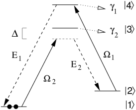
Figure 1: Atoms in a double-$\Lambda$ configuration interacting with two driving fields ($\Omega_{1,2}$) and two generated fields ($E_{1,2}$).

The interacting beams consist of two pump fields with frequencies $\nu_{d1}$ and $\nu_{d2}$ and Rabi-frequencies $\Omega_{1}$ and $\Omega_{2}$, and two generated fields (signal and idler) described by the complex Rabi-frequencies $E_{1}$ and $E_{2}$, with carrier frequencies $\nu_{1}=\nu_{\rm d1}+\omega_{0}$ and $\nu_{2}=\nu_{\rm d2}-\omega_{0}$, where $\omega_{0}=\omega_{\rm 2}-\omega_{\rm 1}$ is the ground-state frequency splitting. It is assumed here that the pump and generated fields are pairwise in two-photon resonance and thus in four-photon resonance. The latter is a consequence of energy conservation. The two photon resonance is a consequence of phase matching and semiclassical treatments show that signal and idler fields are generated precisely at those frequencies. The fields interact via the long-lived coherence on the dipole-forbidden transition between the metastable ground states $|1\rangle$ and $|2\rangle$.

The problem with this model is that associated with the finite detuning $\Delta$, which is necessary to minimize linear absorption, are ac-Stark induced nonlinear phase shifts. These phase shifts reduce conversion efficiency from the pump to the generated modes, and at the same time increase the distance required for conversion to take place johnsson2002 . As was shown in johnsson2002 these problems can be overcome by modifying the system slightly. Instead of the original four-level scheme a five-level set-up depicted in Figure 2 is used. This symmetric configuration cancels ac-Stark shifts. In order to maintain the nonlinear interaction, which is also an odd function of the detuning, it is however necessary to choose atomic states such that the coupling constant for one of the four transitions $|1\rangle\rightarrow|3\rangle$, $|1\rangle\rightarrow|4\rangle$, $|2\rangle\rightarrow|3\rangle$, and $|2\rangle\rightarrow|4\rangle$ has a different sign to the other three. This can easily be accomplished by using different hyperfine levels johnsson2002 .

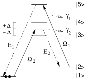
Figure 2: Modified double-$\Lambda$ system. Addition of a fifth level allows the cancellation of destructive phase-shifts.

Choosing the driving field $\Omega_{1}$ to be in resonance with the $|2\rangle\to|5\rangle$ transition while the second driving field $\Omega_{2}$ has a detuning $\pm\Delta$ with $|\Delta|\gg|\Omega_{2}|$ ensures that the linear losses due to single-photon absorption are minimized.

The interaction of the fields with an ensemble of five-level atoms is described by Maxwell’s equations for the fields and a set of density matrix equations for the atoms which determine the atomic polarizations. Under conditions of adiabatic following and for the case of classical fields the latter are ususally solved in steady-state and feed back into the first, yielding nonlinear field equations of motion. This procedure is rather involved, particularly if several atomic levels need to be taken into account, and is completely inadequate for quantized electromagnetic fields. Consequently in this paper we adopt a different procedure.We first derive an effective classical interaction hamiltonian in the adiabatic limit and then quantize the effective theory by replacing the field amplitudes by properly ordered operator expressions.

In order to rigorously calculate the medium response to classical fields, one would have to solve the atomic density matrix equations to all orders in all fields taking into account all relaxation mechanisms. Instead we use a simplified open-system model which allows to derive rather compact expressions for the atomic susceptibilities. In this model the interaction of an individual atom with four classical modes is described by a complex Hamiltonian, which, in a rotating-wave approximation corresponding to slowly-varying amplitudes of the basis $(|1\rangle\;|2\rangle\;|3\rangle\;|4\rangle\;|5\rangle)^{T}$, can be written as

$$H_{\rm int}=-\hbar\left[\begin{matrix}0&0&\Omega_{2}^{*}&\Omega_{2}^{*}&E_{1}^{*}\cr 0&0&E_{2}^{*}&-E_{2}^{*}&\Omega_{1}^{*}\cr\Omega_{2}&E_{2}&-\Delta-i\gamma_{2}&0&0\cr\Omega_{2}&-E_{2}&0&\Delta-i\gamma_{2}&0\cr E_{1}&\Omega_{1}&0&0&-i\gamma_{1}\end{matrix}\right].$$ (1)

At the input the signal and idler modes $E_{1}$ and $E_{2}$ are assumed to have zero amplitude and all atoms are in state $|1\rangle$. Taking into account that optical pumping out of $|1\rangle$ is negligible as $\Delta\gg|\Omega_{2}|$, this is a stable configuration corresponding to an approximate adiabatic eigenstate (to lowest order in $\Delta^{-1}$) of $H$. We now assume that the interaction takes place over sufficiently long time scales, ensuring that the atoms always stay in this approximate adiabatic eigenstate. Under these conditions the Hamiltonian can be replaced by the corresponding eigenvalue $\lambda_{0}$. Solving the 4th order characteristic equations for the eigenvalues of (1) and expanding the solutions in a power series of $(\Omega/\Delta)$, with $\Omega$ being a characteristic value of the Rabi-frequencies, one finds to lowest order

$$H_{\rm int}\longrightarrow\lambda_{0}=\frac{\hbar}{\Delta}\left[\frac{\Omega_{1}^{*}\Omega_{2}^{*}E_{1}E_{2}+\Omega_{1}\Omega_{2}E_{1}^{*}E_{2}^{*}}{|\Omega_{1}|^{2}+|E_{1}|^{2}}\right].$$ (2)

One recognizes two interesting and unusual features. First the eigenvalue and correspondingly the medium polarization cannot be expressed as a polynomial in the field amplitudes. Thus the resonant interaction corresponds to an all-order nonlinear process. Secondly despite the resonant interaction $\lambda_{0}$ has no imaginary component and there are hence no linear losses. This is due to quantum interference associated with EIT. It allows for efficient nonlinear interactions close to resonance without suffering from linear absorption.

To quantize the interaction problem we replace the complex amplitudes of the Rabi-frequencies in (2) by positive and negative frequency components of corresponding operators, choosing normal order in the numerator and the denominator, multiply by the density of atoms and integrate over the interaction volume. We thus arrive at the effective interaction Hamiltonian between the quantized electromagnetic fields

$$\hat{H}_{\rm int}=\frac{\hbar NA}{\Delta}\int\!{\rm d}z\,\left[\frac{\hat{E}_{1}^{\dagger}\hat{E}_{2}^{\dagger}\hat{\Omega}_{1}\hat{\Omega}_{2}+\hat{\Omega}_{1}\hat{\Omega}_{2}\hat{E}_{1}\hat{E}_{2}}{\hat{\Omega}_{1}^{\dagger}\hat{\Omega}_{1}+\hat{E}_{1}^{\dagger}\hat{E}_{1}}\right]$$ (3)

where $N$ is the number density of atoms, $A$ the effective cross section of the beams, and $\hat{E}_{1}(z,t)=d_{51}\sum_{k}\sqrt{{\nu_{1}}/{2\hbar\varepsilon_{0}V}}\,\hat{a}_{1k}(t){\rm e}^{-i(\nu_{k}-\nu_{1})z/c}$ is the slowly varying positive frequency operator of the signal Rabi-frequency. Correspondingly $\hat{\Omega}_{1}(z,t)=d_{52}\sum_{k}\sqrt{{\nu_{d1}}/{2\hbar\varepsilon_{0}V}}\,\hat{b}_{1k}(t){\rm e}^{-i(\nu_{k}-\nu_{d1})z/c}$ denotes the slowly varying positive frequency operator of the first pump Rabi-frequency. The operators $\hat{a}_{\mu}$ and $\hat{b}_{\mu}$ obey harmonic oscillator commutation relations. $V$ is the quantization volume, which shall be identified with the interaction volume and $d_{ij}$ is the dipole matrix element of the $|i\rangle\rightarrow|j\rangle$ transition. It should be noted that numerator and denominator commute and thus there is no ambiguity with respect to the ordering of the two terms.

One can easily verify that there are four independent quantities that commute with $\hat{H}_{\rm int}$ and are therefore constants of motion:

$$\hat{\Omega}_{1}^{\dagger}\hat{\Omega}_{1}+\hat{E}_{1}^{\dagger}\hat{E}_{1} = \,{\rm constant},$$ (4)

$$\hat{\Omega}_{2}^{\dagger}\hat{\Omega}_{2}+\hat{E}_{2}^{\dagger}\hat{E}_{2} = \,{\rm constant},$$ (5)

$$\hat{\Omega}_{1}^{\dagger}\hat{\Omega}_{1}-\hat{\Omega}_{2}^{\dagger}\hat{\Omega}_{2} = \,{\rm constant},$$ (6)

$$\hat{\Omega}_{1}^{\dagger}\hat{\Omega}_{2}^{\dagger}\hat{E}_{1}\hat{E}_{2}+\hat{\Omega}_{1}\hat{\Omega}_{2}\hat{E}_{1}^{\dagger}\hat{E}_{2}^{\dagger} = \,{\rm constant}.$$ (7)

These are the quantum analogs of the classical Manley-Rowe relations which express energy conservation in the system plus an equation expressing the conservation of the relative phase between the fields bloembergen1965 . The existence of these constants of motion will considerably simplify the analysis.

It should be noted that the existence of these constants of motion are not artifacts caused by using an effective rather than the full Hamiltonian. We have also pursued a more rigorous derivation, which involved writing the Heisenberg equations of motion for the atomic and field subsystems seperately and including decay terms. In the limit $\gamma\ll\Delta$ and negligible decay from the two ground states this approach also yields (4) – (6). Unfortunately the equations of motion obtained in this way have a number of unpleasant features and are not ameanable to analytic solution, which is why we have chosen to use the effective Hamiltonian (3) as the starting point of our discussion.

III Classical solutions for forward four-wave mixing

To obtain classical solutions we use (3), and note that the polarization $P$ of the medium for the probe transitions can be expressed as a partial derivative of the average single-atom interaction energy with respect to the electric field or, respectively, the Rabi-frequencies $E_{i}$

$$P_{i}=-\frac{Nd_{i}}{\hbar}\left\langle\frac{\partial{H}_{\rm int}}{\partial E_{i}^{*}}\right\rangle\,{\rm e}^{-i\nu_{i}(t-z/c)}+c.c.,\quad i=1,2$$ (8)

A similar expression holds for the drive field polarizations. Here $\left\langle...\right\rangle$ denotes quantum-mechanical averaging, $d_{i}$ the dipole matrix elements of the corresponding transition and $N$ is the atom density. Hence one can directly obtain the stationary field equations in slowly-varying amplitude and phase approximation:

$$\frac{{\rm d}E_{i}}{{\rm d}z}=-i\frac{\eta_{i}}{\hbar}\left\langle\frac{\partial{H}_{\rm int}}{\partial E_{i}^{\ast}}\right\rangle,$$ (9)

where $\eta_{i}=Nd_{i}^{2}\omega_{i}/(2\hbar c\epsilon_{0})$. This approach allows us to obtain the polarizations and equations of motion for the fields without calculating the density matrix hamiltonian .

Using (9), going to a comoving frame via the transformation $(z,t)\to(\zeta=z,\tau=t-z/c)$, assuming that all dipole moments (averaged over orientations of the atoms) are approximately the same and introducing the common coupling coefficient $\kappa=N\overline{\,d_{i}^{2}\,}\omega_{i}/(2\hbar c\epsilon_{0})=3N\lambda^{2}\gamma/8\pi$, gives the following equations of motion for the fields:

$$\frac{\partial}{\partial\zeta}E_{1} = -i\kappa\frac{\Omega_{1}^{\ast}\Omega_{1}^{2}\Omega_{2}E_{2}^{\ast}-E_{1}^{2}E_{2}\Omega_{1}^{\ast}\Omega_{2}^{\ast}}{\Delta\left(|\Omega_{1}|^{2}+|E_{1}|^{2}\right)^{2}},$$ (10)

$$\frac{\partial}{\partial\zeta}E_{2} = -i\kappa\frac{\Omega_{1}\Omega_{2}E_{1}^{\ast}}{\Delta\left(|\Omega_{1}|^{2}+|E_{1}|^{2}\right)},$$ (11)

$$\frac{\partial}{\partial\zeta}\Omega_{1} = i\kappa\frac{\Omega_{1}^{2}\Omega_{2}E_{1}^{*}E_{2}^{*}-|E_{1}|^{2}E_{1}E_{2}\Omega_{2}^{*}}{\Delta\left(|\Omega_{1}|^{2}+|E_{1}|^{2}\right)^{2}},$$ (12)

$$\frac{\partial}{\partial\zeta}\Omega_{2} = -i\kappa\frac{E_{1}E_{2}\Omega_{1}^{*}}{\Delta\left(|\Omega_{1}|^{2}+|E_{1}|^{2}\right)}.$$ (13)

Without sacrificing the underlying physics we can assume that the intial intensities of the pump fields and the intial intensities of the generated fields are equal:

$$|\Omega_{1}|^{2}=|\Omega_{2}|^{2},\;\;\;\;|E_{1}|^{2}=|E_{2}|^{2}.$$ (14)

As can easily be seen, the constants of motion imply that asymmetric initial conditions lead to exactly the same dynamics with the intensities merely shifted up or down by a constant.

Introducing a normalized intensity $y(t)$ with the identification $\zeta\to t$

$$y(t) = \frac{|\Omega_{1}(t)|^{2}}{|\Omega_{1}|^{2}+|E_{1}|^{2}},$$ (15)

$$\dot{y}(t) = -2\frac{\kappa}{\Delta}\,\frac{{\rm Im}\bigl{(}\Omega_{1}\Omega_{2}E_{1}^{*}E_{2}^{*}\bigr{)}}{\bigl{(}|\Omega_{1}|^{2}+|E_{1}|^{2}\bigr{)}^{2}}$$ (16)

and making use of the constants of motion (4) – (6) to reduce the problem to one variable, we obtain the differential equation

$$\frac{(\Delta/\kappa)^{2}}{2}\frac{{\rm d^{2}}y}{{\rm d}t^{2}}=\frac{\rm d}{{\rm d}y}\Bigl{(}4y^{2}(y-1)^{2}\Bigr{)}.$$ (17)

In this form it is clear that the normalized intensity of the drive field can be identified with a particle of mass $m=\Delta/\kappa$ moving in the potential $V(y)=-4y^{2}(y-1)^{2}$, depicted in Figure 3. Conservation of energy requires that the particle be trapped between $0\leq y\leq 1$. If $E_{1}(0)=E_{2}(0)=0$, i.e. there is no seeding of the generated fields, then we have the case where $y(0)=1$. As is clear from the potential diagram, this corresponds to a point of unstable equilibrium, and indicates that no dynamics can take place.

Choosing to seed the generated fields with a specific amplitude and phase corresponds to moving the particle off the critical point in the potential diagram. The drive field intensity will then oscillate, transferring energy back and forth between the drive and generated fields according to the constants of motion. The dynamics is however sensitive to both the strength of the seed fields and the initial relative phase between all four fields. The exact analytical solution shows that the oscillation period of the energy transfer as well as the maximum conversion efficiency depend on the seed-field intensity and phase korsunsky1999 ; johnsson2002 .

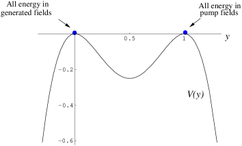
Figure 3: Nonlinear pendulum potential experienced by a “particle” corresponding to the exchange energy between the pump and generated fields. $\kappa/\Delta$ taken to be unity.

IV Quantum theory of stationary forward four-wave mixing

IV.1 Exact numerical solution to the stationary quantum problem

While forward four-wave mixing is relatively well understood in the semiclassical case, very little work has been done on the fully quantum case, that is, where both the atomic subsystem and the interacting electromagnetic fields are quantized. There are at least three reasons for considering such a formulation.

First, from (10) – (13) we see that the nonlinear interaction of the system actually increases as the strength of the pump fields is reduced. However, when the strength is reduced to a level corresponding to only a few photons, the semiclassical approximations must fail. Nonetheless, the extreme nonlinearities experienced in conditions of very weak fields opens the intriguing possibility of nonlinear effects at the few-photon level.

Secondly, a semiclassical analysis is not able to cope with the physically realistic situation where initially only two fields are present. Vacuum seeding through quantum fluctuations cannot be described in the semiclassical framework, and one must always introduce at least a third field into the analysis so that conversion can take place.

Thirdly, the behaviour of the system, at least in a semiclassical analysis, is extremely sensitive to variations in intial phase and amplitude of the pump and seed fields. When the fields are treated quantum mechanically, these parameters will often be indeterminate, particularly when starting from a vacuum field.

While an analytic solution of the fully quantum case appears intractable, it is nevertheless possible to obtain exact solutions numerically under stationary conditions. The stationary spatial evolution of the fields can be described by considering the time evolution of four harmonic oscillators $\hat{a}_{1},\hat{a}_{2}$ and $\hat{b}_{1},\hat{b}_{2}$ corresponding to the generated and pump fields respectively, interacting via the nonlinear Hamiltonian

$$\hat{H}_{\rm int}=\frac{\hbar\kappa c}{\Delta}\biggl{[}\frac{\hat{b}_{1}^{\dagger}\hat{b}_{2}^{\dagger}\hat{a}_{1}\hat{a}_{2}+\hat{a}_{1}^{\dagger}\hat{a}_{2}^{\dagger}\hat{b}_{1}\hat{b}_{2}}{\hat{b}_{1}^{\dagger}\hat{b}_{1}+\hat{a}_{1}^{\dagger}\hat{a}_{1}}\biggr{]}$$ (18)

with the following identification $\hat{E}_{i}\to\hat{a}_{i}$, $\hat{\Omega}_{i}\to\hat{b}_{i}$ and $\kappa=3N\lambda^{2}\gamma/8\pi$.

The technique we use is to describe the possible states of the system in a number state basis of the fields, use the effective Hamiltonian (18) and solve the resulting Schrödinger equation numerically. We will use the notation $|n_{\Omega_{1}}\;n_{\Omega_{1}}\;n_{E_{1}}\;n_{E_{2}}\rangle$ for our basis vectors, where $n_{\Omega_{1}}$ is the number of photons in the $\Omega_{1}$ mode, $n_{\Omega_{2}}$ is the number of photons in the $\Omega_{2}$ mode and so on.

The difficulty with this technique is that even though we have eliminated the atomic degrees of freedom by using an effective Hamiltonian, because we are considering a four-wave mixing process the size of the Hilbert space will scale as $n^{4}$, where $n$ is a characteristic number of photons in each of the fields. Consequently, if we wished to consider, say, 100 photons in each of the beams, our Hilbert space would be $10^{8}$ dimensional, and the problem would involve diagonalizing matrices with $10^{16}$ elements. Thus, as it stands, this approach is not computationally feasible.

The scaling problem can be avoided by using the constants of motion (4) – (6). Taken together, these relations allow us to reduce a problem with four degrees of freedom to just one, which is essentially the energy transfer from one field to another. For example, (5) states that when a photon is annihilated in the $\Omega_{1}$ mode, another must be created in the $E_{1}$ mode. Reduction of the problem to one with a single degree of freedom allows us to choose the basis

$$\Psi_{nm}=\bigl{|}n_{1}-n\;\,\,n_{2}-n\;\,\,n_{3}+n\;\,\,n_{4}+n\bigr{\rangle}$$ (19)

where $n_{1}$, $n_{2}$, $n_{3}$ and $n_{4}$ denote the number of photons initially in each of the four modes, and $n$ is the single degree of freedom denoting how many photons have been transferred out of the pump mode.

IV.2 Intensity evolution and quantum limitation of conversion efficiency

We first consider the evolution of the fields when the initial states of the pump fields are given by number states. This situation is computationally easy, and we have calculated results for initial states consisting of up to several thousand photons. A number state consisting of several thousand photons, however, is not particularly experimentally realistic, and thus here we consider only low photon numbers. The results are shown in Figure 4.

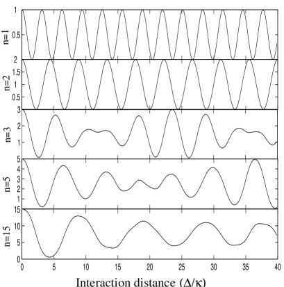
Figure 4: Evolution of average pump photon number from initial number states. From top to bottom the initial photon number in the pump modes are 1, 2, 3, 5 and 15 photons.

We note that the solutions are oscillatory, in qualitative analogy to the semiclassical predictions. In the fully quantum case, however, we see that only when the initial pump fields contain one or two photons are the oscillations comprised of just one frequency. If the initial fields contain three or more photons several oscillation frequencies are present, leading to a reduced conversion efficiency. Provided long enough interaction distances are considered, however, the different oscillation frequencies come back into phase and reinforce each other, leading to the conclusion that complete conversion can always be obtained at some point.

Another point to note is that as the intensity of the initial pump fields is increased, the oscillation period increases. This is in agreement with the form of the Hamiltonians (3), (18). The denominator is a constant of motion and is related to the intensity of the pump field $\Omega_{1}$. Thus a more intense pump field gives a smaller interaction energy and consequently a longer conversion distance.

Next we consider the case where the pump fields are initially described by coherent states. This situation is considerably more computationally intensive, but calculations with an average photon number of up to 1000 in each pump mode have been carried out. The results are shown in Figure 5.

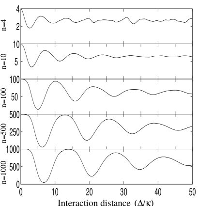
Figure 5: Evolution of average pump photon number for coherent initial states. From top to bottom: an average photon number of 4, 10, 100, 500 and 1000.

There are several overall qualitative features.

We see oscillations on a short distance scale damping out over a longer distance scale to a conversion efficiency of approximately one third. The damping at longer distances can be explained by considering a coherent state to be superposition of number states. Each number state has a different oscillation period, and consequently interfere with each other and get out of phase. As would be expected, on still longer distance scales fractional revivals are seen. As the input power is increased, the conversion distance (distance to the first mininum in pump field intensity) increases logarithmically while the conversion efficiency asymptotically approaches unity. The scaling of the conversion distance with input power in the resonantly enhanced four-wave mixing scheme is exactly opposite to the case of ordinary off-resonant four-wave mixing. There the conversion distance decreases with increasing input power.

IV.3 Quantum correlations and fluctuations of the generated fields

We now discuss the quantum fluctuations and correlations of the generated fields. It is immediately evident from the interaction Hamiltonian that when the two generated fields start in the vacuum state, they will at all times be perfectly photon-number correlated. Only states with equal photon number in both modes can be generated. Consequently the intensity difference between the two fields is perfectly squeezed:

$$\left\langle\Delta\bigl{(}\hat{a}_{1}^{\dagger}\hat{a}_{1}-\hat{a}_{2}^{\dagger}\hat{a}_{2}\bigr{)}^{2}\right\rangle\equiv 0.$$ (20)

To characterize the statistics of photon pairs in the two generated modes we have calculated the $Q$-parameter for different input states and intensities. As can be seen from Figure 6 the pair statistics remain sub-Possonian ($Q\leq 0$) for a Fock-state input with $n\leq 2$. For a Fock-state input with $n>2$ the pair statistics have a sub-Poissonian character only for very small interaction distances and around the revival of the input intensity (see Fig. 4).

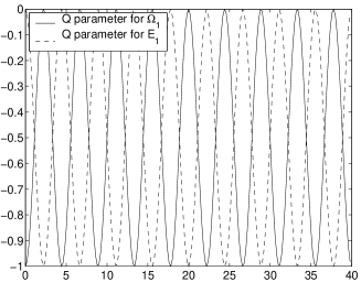
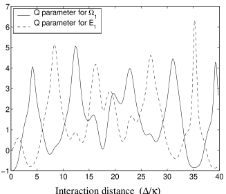
Figure 6: Mandel $Q$ parameter for initial Fock states with $n=2$ (top) and $n=10$ (bottom) in both pump modes. Dashed line shows $Q$ parameter for generated fields, full line for pump fields.

For an initial coherent state the pair statistics remain super-Poissonian at all times. This is illustrated in Figure 7.

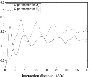
Figure 7: Mandel $Q$ parameter for initial coherent states with $\langle n\rangle=10$ in both pump modes. Dashed line shows $Q$ parameter for generated fields, full line for pump fields.

IV.4 Realization of phase gate for continuous-variable quantum computation

The field evolution from an initial Fock state with $n=1$ photons in each of the pump modes, discussed in subsection IV.2, exhibits an interesting feature. After a single complete cycle of energy conversion to the generated fields and back, the quantum state of the system undergoes a phase change of exactly $\pi$. This can be used to implement a phase gate for continuous quantum computation. Noting that no conversion occurs unless both input modes are excited and fixing the medium length at a value corresponding to twice the conversion length for a single photon input of both pump modes one has the following evolution of states

$$|0,0,0,0\rangle \longrightarrow |0,0,0,0\rangle,$$

$$|1,0,0,0\rangle \longrightarrow |1,0,0,0\rangle,$$

$$|0,1,0,0\rangle \longrightarrow |0,1,0,0\rangle,$$ (21)

$$|1,1,0,0\rangle \longrightarrow -|1,1,0,0\rangle.$$

This is a perfect realization of a phase gate.

V Mean-field theory of resonant forward four-wave mixing

In order to obtain a better understanding of the quantum dynamics of resonant four-wave mixing, in particular the limitations and scaling of conversion efficiency as well as the conversion distance, we now derive approximate analytical solutions within an appropriate mean-field theory. Our starting point is again the effective Hamiltonian (18), along with the assumption that we can replace the denominator, a constant of motion, with its expectation value. In this case the equations of motion for the fields in the Heisenberg picture are

$$\frac{\rm d}{{\rm d}t}\hat{b}_{1} = -\frac{i\kappa c}{\Delta d}\;\hat{b}_{2}^{\dagger}\hat{a}_{1}\hat{a}_{2}$$ (22)

$$\frac{\rm d}{{\rm d}t}\hat{a}_{1} = -\frac{i\kappa c}{\Delta d}\;\hat{a}_{2}^{\dagger}\hat{b}_{1}\hat{b}_{2}$$ (23)

$$\frac{\rm d}{{\rm d}t}\hat{b}_{2} = -\frac{i\kappa c}{\Delta d}\;\hat{b}_{1}^{\dagger}\hat{a}_{1}\hat{a}_{2}$$ (24)

$$\frac{\rm d}{{\rm d}t}\hat{a}_{2} = -\frac{i\kappa c}{\Delta d}\;\hat{a}_{1}^{\dagger}\hat{b}_{1}\hat{b}_{2}$$ (25)

where $d=\langle\hat{b}_{1}^{\dagger}\hat{b}_{1}+\hat{a}_{1}^{\dagger}\hat{a}_{1}\rangle$.

The equations of motion for the average field intensities $\langle\hat{b}_{1}^{\dagger}\hat{b}_{1}\rangle$ and so on will contain four-field correlation functions, for example

$$\frac{\rm d}{{\rm d}\zeta}\langle\hat{b}_{1}^{\dagger}\hat{b}_{1}\rangle=\frac{i\kappa}{\Delta d}\left[\langle\hat{b}_{1}\hat{b}_{2}\hat{a}_{1}^{\dagger}\hat{a}_{2}^{\dagger}\rangle-\langle\hat{a}_{1}\hat{a}_{2}\hat{b}_{1}^{\dagger}\hat{b}_{2}^{\dagger}\rangle\right]$$ (26)

where we have once again switched to a spatial rather than a temporal picture.

To proceed further we assume that all fields are gaussian and that correlations between pump and generated fields can be neglected. This assumption is reasonable as long as the pump fields are initially in coherent states with sufficiently large amplitude. With this decorrelation approximation, the fourth order expectation values can be expressed as sets of bilinear terms of the form $\langle\hat{b}_{i}^{\dagger}\hat{b}_{j}\rangle$ and $\langle\hat{a}_{i}^{\dagger}\hat{a}_{j}\rangle$. It is important that we also keep anomalous correlations, such as $\langle\hat{a}_{i}\hat{a}_{j}\rangle$, as both pairs of fields are strongly correlated. In addition, we can use the constants of motion (4) – (6) to relate the expectation values of the number operators $\langle\hat{b}_{1}^{\dagger}\hat{b}_{1}\rangle$, $\langle\hat{b}_{2}^{\dagger}\hat{b}_{2}\rangle$, $\langle\hat{a}_{1}^{\dagger}\hat{a}_{1}\rangle$ and $\langle\hat{a}_{2}^{\dagger}\hat{a}_{2}\rangle$.

If we define $\langle\hat{b}_{1}\hat{b}_{2}\rangle=b_{12}e^{i\varphi_{b}}$, $\langle\hat{a}_{1}\hat{a}_{2}\rangle=a_{12}e^{i\varphi_{a}}$, and $\langle\hat{b}_{1}^{\dagger}\hat{b}_{1}\rangle=b$, then we obtain the following set of coupled, complex-valued nonlinear differential equations:

$$\frac{\rm d}{{\rm d}\zeta}a_{12} = \frac{\kappa}{\Delta d}(2a+1)a_{12}\sin(\varphi_{a}-\varphi_{b})$$ (27)

$$\frac{\rm d}{{\rm d}\zeta}a_{12} = \frac{\kappa}{\Delta d}(2b-2d-1)b_{12}\sin(\varphi_{a}-\varphi_{b})$$ (28)

$$\frac{\rm d}{{\rm d}\zeta}b = \frac{2\kappa}{\Delta d}b_{12}E_{12}\sin(\varphi_{a}-\varphi_{b})$$ (29)

$$\frac{\rm d}{{\rm d}\zeta}\varphi_{b} = -\frac{\kappa}{\Delta d}(2b+1)\frac{a_{12}}{b_{12}}\cos(\varphi_{a}-\varphi_{b})$$ (30)

$$\frac{\rm d}{{\rm d}\zeta}\varphi_{a} = \frac{\kappa}{\Delta d}(2b-2d-1)\frac{b_{12}}{a_{12}}\cos(\varphi_{a}-\varphi_{b}).$$ (31)

To simplify this system we note that if we take expectation values of both sides of (7) we find $b_{12}a_{12}\cos(\varphi_{a}-\varphi_{b})$ is a constant of motion. If we assume that both generated fields start from vacuum this constant is equal to zero, and since $b_{12}$ and $a_{12}$ are not always zero we see that $\cos(\varphi_{a}-\varphi_{b})=\pm 1$, with the sign flip coming at the end of each conversion cycle. This observation, in conjunction with two more constants of motion that can be extracted from (27) – (31), enable us to reduce the set of five coupled equations to just one:

$$\frac{{\rm d}b}{\rm d\zeta}=\frac{2\kappa}{\Delta b_{0}}\sqrt{(b^{2}+b-b_{0})(b-b_{0})(b-b_{0}-1)},$$ (32)

where $b_{0}=\langle\hat{b}_{1}^{\dagger}(0)\hat{b}_{1}(0)\rangle=\langle\hat{b}_{2}^{\dagger}(0)\hat{b}_{2}(0)\rangle$. This is the equation governing the evolution of the expectation value of the number of photons in each of the pump modes, under the assumption that both pump fields have the same intensity and the two generated fields start from vacuum.

As a fourth order polynomial is involved, this differential equation can be (implicitly) solved analytically in terms of elliptic integrals, but the specific form of the solution is involved and not particularly illuminating. Numerical solutions to (32) are plotted in Figure 8 for a number of initial pump field intensitities.

Figure 8: Pump field intensity in the mean-field approximation. From top to bottom: 10, 50, 100, 500 and 1000 photons. $\kappa/\Delta=1$, $b_{0}=10$.

One recognizes an oscillatory exchange of energy with a non-perfect conversion effiency. Comparison of the mean-field results with the fully quantum calculation for the case of a coherent pump input shows good agreement over the first period of energy exchange between pump and generated fields (Figure 9). In particular the maximum conversion efficiency and the conversion distance are well reproduced. As in the quantum solutions, the conversion period increases logarithmically with the input intensity. For larger distances the mean-field solution remains periodic, while the oscillations in the true quantum case decay. As the interaction distance increases, higher order correlations build up and thus the gaussian factorization approximation used in the mean-field theory breaks down.

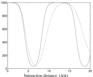
Figure 9: Comparison between the exact numerical solutions (dashed line) and the mean-field theory (solid line) for a coherent state with an average photon number of 1000.

Analoguous to the semiclassical case, (32) can be mapped to a nonlinear pendulum problem, with $b$ corresponding to the position of a particle with mass $\Delta^{2}/\kappa^{2}$ moving in a potential

$$V(b)=-\frac{2}{b_{0}^{2}}(b^{2}+b-b_{0})(b-b_{0})(b-b_{0}-1)$$ (33)

where $b$ plays the role of the particle position and the identification $\zeta\to t$ is used.

The potential (33) is plotted in Figure 10 for the case $b_{0}=10$, $\kappa/\Delta=1$.

Figure 10: Nonlinear pendulum potential experienced by a “particle” whose position corresponds to the number of photons in the pump modes. $\kappa/\Delta=1$, $b_{0}=10$.

From the shape of the potential one can see that different dynamics is expected compared with the semiclassical case, where the potential is described by Figure 3. In the semiclassical analysis, choosing the initial intensity of $a_{1}$ and $a_{2}$ to be zero corresponds to starting exactly on the right hand peak of the potential in Figure 3, and consequently no dynamical evolution can occur.

In the mean-field theory, however, the starting position ($b_{0})$ is always slightly to the left of the right summit (peak position is $\sim b_{0}+\frac{1}{2}$ for large $b_{0}$), and consequently oscillation will always take place. As the input power is increased the starting position asymptotically approaches the right hand peak, but never reaches it. From the potential (33) one can easily obtain the conversion distance or oscillation period:

$$z_{\rm conv}=\int_{b_{0}}^{b_{1}}\!\!\frac{{\rm d}b}{\sqrt{-\frac{2\Delta}{\kappa}V(b)}}$$ (34)

where $b_{1}$ is the inner turning point. As the input power is increased, it takes longer for the oscillation to begin due to the flatter gradient of the potential, leading to the logarithmic increase in conversion period. This is in sharp contrast to ordinary off-resonance four-wave mixing, where the conversion length decreases with input power. The effective hamiltonian discussed in the present paper can be converted into that of ordinary off-resonant four-wave mixing by replacing the intensity dependent denominator $d$ by a constant. Figure 11 gives a comparision of the conversion distance as a function of input power for the two cases. The periods were found from numerical solutions to the full quantum problem using the Hamiltonian (3) with and without the resonant denominator.

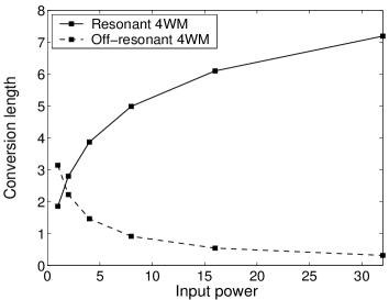
Figure 11: Scaling of conversion distance as function of input intensity of coherent pump for ordinary off-resonance four-wave mixing (dashed line, $d=$ const.) and resonant four-wave mixing (full line).

One clearly recognizes the peculiar feature of the resonant process to work better for smaller input intensities.

From the roots of (33) one can immediately obtain a result connecting input intensity and conversion efficiency. Defining the conversion efficiency $e=b_{\textrm{min}}/b_{0}$ we find

$$e=1-\frac{1}{2b_{0}}(\sqrt{4b_{0}+1}-1)\sim 1-\frac{1}{\sqrt{b_{0}}}.$$ (35)

Thus in the mean-field model the conversion efficiency $(1-e)$ scales with the input pump field as $b_{0}^{-1/2}$.

VI summary

In the present paper we have discussed the quantum theory of stationary resonant four-wave mixing in a forward scattering configuration. We considered the interaction of four electromagentic fields with atoms in a modified double-$\Lambda$ configuration. The modified five-state coupling scheme was used instead of the standard four-level one in order to eliminate ac-Stark induced nonlinear phase shifts johnsson2002 . This is necessary, because a full quantum analysis shows that full conversion cannot be obtained when these terms are present, even in the asymptotic limit — 50% conversion is the best that can be achieved using coherent states.

To eliminate the atomic variables we assumed adiabatic following and derived a classical nonlinear interaction Hamiltonian of the four electromagnetic fields. In contrast to ordinary off-resonant four-wave mixing, the denominator of this Hamiltonian contains the sum of the intensities of the resonant pair of pump and generated fields. This is a consequence of the infinitely long-lived two-photon resonance which is entirely determined by power-broadening for arbitrarily small field intensities. As a consequence the effective Hamiltonian cannot be expanded as a power series in the fields and the nonlinear interaction becomes stronger the smaller the pump field intensity. The classical evolution can be mapped onto a one-dimensional nonlinear pendulum and solved exactly, provided small seed fields are included in the analysis. The initial evolution of the generated fields from vacuum, however, is entirely determined by quantum fluctuations and thus cannot be described within a classical approach.

To obtain a full quantum solution under stationary conditions we quantized the effective interaction Hamiltonian by replacing c-number expressions by properly ordered operator products. We showed that the constants of motion of the Hamiltonian allow us to reduce the stationary wave mixing process to a single-mode problem, which can be solved numerically for up to $10^{3}$ input photons. We have analyzed the field evolution starting from initial Fock and coherent states in the pump modes. In both cases an oscillatory energy exchange between the modes was found. For the case of initial Fock states with up to $n=2$ photons in both pump modes, the oscillation is purely sinusoidal with a single frequency and complete conversion is possible. For higher input photon numbers multiple frequencies appear and complete conversion is only possible after several oscillation periods. In the case of coherent input fields the oscillations in the energy exchange are damped and complete conversion can be achieved only asymptotically for large input intensities.

As the four-wave mixing process simultaneously creates photons in two modes, the photon numbers in those modes are perfectly quantum correlated, which has potential applications in quantum communication systems. The statistics of the photon pair production is, however, mostly super-Poissonian.

We observed an interesting property of the four-wave mixing process when the two input fields are both in a single-photon Fock state. After a complete conversion cycle into the generated fields and back the quantum state attains a phase shift of exactly $\pi$. This allows one to construct an ideal phase gate for continuous variable quantum computation.

In order to gain more physical insight in the quantum four-wave mixing we developed a mean-field theory assuming gaussian and independent pump and generated fields but taking into account anomalous field correlations. The mean-field equations can again be mapped to a one-dimensional anharmonic pendulum and solved exactly. The solutions for the average intensities reproduce the quantum results for coherent input over the first oscillation period. In particular analytic expressions for the conversion length and the conversion efficiency can be derived which coincide very well with the exact results.

References

- (1) S. E. Harris, Physics Today 50, 36 (1997).
- (2) M. D. Lukin and A. Imamoglu, Nature 413, 273 (2001).
- (3) J. P. Marangos, Journal of Modern Optics 45, 471 (1998).
- (4) S. E. Harris, J. E. Field, and A. Imamoglu, Phys. Rev. Lett. 64, 1107 (1990).
- (5) K. Hakuta, L. Marmet, and B.P. Stoicheff, Phys. Rev. Lett. 66, 596 (1991); G.Z. Zhang, K. Hakuta, and B.P. Stoicheff, Phys. Rev. Lett.71, 3009 (1993).
- (6) M. Jain, H. Xia, G.Y. Yin, A.J. Merriam, and S.E. Harris, Phys. Rev. Lett. 77, 4326-4329 (1996); S.E. Harris, G.Y. Yin, M. Jain, H. Xia, and A.J. Merriam, Phil. Trans. R. Soc. Lond. A 355, 2291-2304 (1997).
- (7) S. E. Harris and Y. Yamamoto, Phys. Rev. Lett. 81, 3611 (1998).
- (8) S. E. Harris and L. V. Hau, Phys. Rev. Lett. 82, 4611 (1999).
- (9) M. D. Lukin and A. Imamoglu, Phys. Rev. Lett. 84,1419 (2000).
- (10) H. Schmidt and A. Imamoglu, Opt. Lett. 21, 1936 (1996).
- (11) P.R. Hemmer, K. Z. Cheng, J. Kierstead, M. S. Shariar, and M. K. Kim, Opt. Lett. 19, 296 (1994); B. S. Ham, M. S. Shariar, M. K. Kim, and P. R. Hemmer, Opt. Lett. 22, 1849 (1997).
- (12) S. Babin, U. Hinze, E. Tiemann, B. Wellegehausen, Opt. Lett. 21, 1186 (1996); S. Babin, E. V. Podivilov, D.A. Shapiro, U. Hinze, E. Tiemann, B. Wellegehausen, Phys. Rev. A 59, 1355 (1999); U. Hinze, L. Meyer, B.N. Chichkov, E. Tiemann, B. Wellegehausen, Opt. Comm 166, 127 (1999).
- (13) M. D. Lukin, M. Fleischhauer, A.S. Zibrov, H.G. Robinson, V.L. Velichansky, L. Hollberg, M.O. Scully, Phys. Rev. Lett. 79, 2959 (1997).
- (14) A. K. Popov, S. A. Myslivets, Kvant. Elektr. 24, 1033 (1997).
- (15) B. Lu, W.H. Burkett, M. Xiao, Opt. Lett. 23, 804 (1998).
- (16) E. A. Korsunsky and D. V. Kosachiov, Phys. Rev. A 60, 4996 (1999).
- (17) E. A. Korsunsky and M. Fleischhauer, preprint quant-ph/0204089.
- (18) M. D. Lukin, P. Hemmer, M. Loeffler, and M. O. Scully, Phys. Rev. Lett. 81, 2675 (1998).
- (19) M. D. Lukin, P. R. Hemmer, M. O. Scully, in Adv. At. Mol. and Opt. Physics, 42B, 347 (Academic Press, Boston, 1999).
- (20) M. Fleischhauer in Frontiers of Laser Physics and Quantum Optics, (Z. Xu, S. Xie, S.-Y. Zhu and M. O. Scully, Eds.), p. 97-106 (Springer, Berlin, 2000).
- (21) A. S. Zibrov, M. D. Lukin and M. O. Scully, Phys. Rev. Lett. 83, 4049 (1999).
- (22) H. P. Yuen and J. H. Shapiro, Opt. Lett. 4, 334 (1979).
- (23) N. Bloembergen, Nonlinear Optics (W. A. Benjamin, New York 1965).
- (24) R. W. Boyd, Nonlinear Optics (Academic Press, San Diego 1992).
- (25) M. D. Lukin, A. B. Matsko, M. Fleischhauer, and M. O. Scully, Phys. Rev. Lett. 82, 1847 (1999)
- (26) M. Fleischhauer, M. D. Lukin, A. B. Matsko, and M. O. Scully, Phys. Rev. Lett. 84, 3558 (2000).
- (27) Mattias Johnsson, Evgeny Korsunsky and Michael Fleischhauer, preprint quant-ph/0205194
- (28) the approach is adapted from: A. O. Melikyan and S. G. Saakyan, Zh. Exp.Teor. Fiz. 76, 1530 (1979) [Sov. Phys. JETP 49, 776 (1979)]; A. R. Karapetyan and B. V. Kryzhanovskii, Zh. Exp. Teor. Fiz. 99, 1103 (1991) [Sov. Phys. JETP 72, 613 (1991)]; B. Kryzhanovsky and B. Glushko, Phys. Rev. A 45, 4979 (1992).