On first-arrival-time distributions for a Dirac electron in 1+1 dimensions

Abstract

For the special case of freely evolving Dirac electrons in $1\;+\;1$ dimensions, Feynman checkerboard paths have previously been used to derive Wigner’s arrival-time distribution which includes all arrivals. Here, an attempt is made to use these paths to determine the corresponding distribution of first-arrival times. Simple analytic expressions are obtained for the relevant components of the first-arrival propagator. These are used to investigate the relative importance of the first-arrival contribution to the Wigner arrival-time distribution and of the contribution arising from interference between first and later (i.e. second, third, … ) arrivals. It is found that a distribution of (intrinsic) first-arrival times for a Dirac electron cannot in general be consistently defined using checkerboard paths, not even approximately in the nonrelativistic regime.

I Introduction

In the past decade there has been considerable interest in deriving and understanding arrival-time distributions for quantum particles, using a wide variety of approaches (for recent reviews see rev1 ; rev2 ; MSE02 ). Here we focus on an approach based on Feynman paths feynman .

Yamada and Takagi yam1 ; yam2 applied the consistent histories approach, with Feynman paths as particle histories, to the problem of deriving an intrinsic arrival-time distribution. They considered the special case of a freely evolving nonrelativistic quantum particle in one spatial dimension. In yam1 they showed that within their approach one cannot classify the histories according to the number of times $n$ that a particle arrives at a given spatial point $x=X$ during a specified finite time interval because the amplitude for $n$ arrivals is zero for every finite $n$. Their qualitative explanation was that a typical Feynman path, being nondifferentiable in time, intersects $X$ an infinite number of times in the given time interval, leaving zero amplitude for any finite value of $n$. They further suggested that this would also be the case for a quantum particle propagating in three spatial dimensions in the presence of a potential.

The velocity associated with a typical Feynman path for a nonrelativistic electron is infinite at almost every point on it. This is not the case for a relativistic electron – the velocity associated with a Feynman path feynman ; JS for a nonrelativistic electron is infinite at almost every point on it. Hence, such a path will not intersect $X$ an infinite number of times in a given finite time interval and the amplitude for $n$ arrivals need not be zero for every finite $n$. This is the primary motivation for the following attempt to derive the first-arrival-time distribution for a freely evolving Dirac electron in $1+1$ dimensions. In Sec II, a checkerboard path derivation crl of Wigner’s arrival-time distribution Wigner which includes all arrivals is sketched, primarily to introduce the basic notation and concepts used in the following sections. In Sec. III the first-arrival propagator for this special case is derived. Unfortunately, there is interference between the $n=1$ and $n>1$ contributions to the arrival-time distribution so that the distribution of intrinsic first-arrival times cannot be consistently defined using this approach. Calculated results for the $n=1$ and interference contributions are presented in Sec. IV for two simple cases. Concluding remarks are made in Sec. V.

II Checkerboard Paths and Wigner’s arrival-time distribution for Dirac electrons

Consider the $1+1$ dimensional free-electron Dirac equation in the form

$$i\hbar\hat{1}\frac{\partial}{\partial t}\Psi(x,t)\>=\>\hat{H}\Psi(x,t)\>=\>-i\hbar c\hat{\sigma}_{z}\frac{\partial}{\partial x}\Psi(x,t)\>-\>mc^{2}\hat{\sigma}_{x}\Psi(x,t)$$ (1)

with $\Psi(x,t)\>\equiv\>\bigl{(}\Psi_{+}(x,t),\Psi_{-}(x,t)\bigr{)}^{T}$ a two-component spinor and

$$\hat{\sigma}_{x}\>=\>\left(\matrix{0&1\cr 1&0}\right)\;\;,\;\;\hat{\sigma}_{z}\>=\>\left(\matrix{1&0\cr 0&-1}\right)\;\;.$$ (2)

The velocity operator

$$\hat{v}\>\equiv\>\frac{d\hat{x}}{dt}\>=\>\frac{i}{\hbar}\>[\hat{H},\hat{x}]\;=\>c\>\hat{\sigma}_{z}$$ (3)

has the orthonormal eigenfunctions

$$\chi_{{}_{+}}\>=\>\left(\matrix{1\cr 0}\right)\;\;,\;\;\chi_{{}_{-}}\>=\>\left(\matrix{0\cr 1}\right)$$ (4)

with eigenvalues $+c$ and $-c$ respectively. Hence,

$$\Psi(x,t)\>=\>\left(\matrix{\Psi_{+}(x,t)\cr\Psi_{-}(x,t)}\right)\>=\>\Psi_{+}(x,t)\;\chi_{+}+\Psi_{-}(x,t)\;\chi_{-}$$ (5)

and the upper and lower components of the wave function $\Psi(x,t)$ are, respectively, the amplitudes at ($x,t$) for the right-going ($+c$) and left-going ($-c$) velocity eigenstates $\chi_{+}$ and $\chi_{-}$. The four components of the retarded $2\times 2$ propagator $K(x_{B},t_{B};x_{A},t_{A})\equiv K(B;A)$ of the $1+1$ dimensional free-electron Dirac equation (1) are labelled by velocity directions ($+$ or $-$) at $(x_{A},t_{A})$ and at $(x_{B},t_{B})$ and are accordingly defined by

$$\left(\matrix{\Psi_{+}(x_{B},t_{B})\cr\Psi_{-}(x_{B},t_{B})}\right)\>=\>\int_{-\infty}^{\infty}dx_{A}\left(\matrix{K_{++}(x_{B},t_{B};x_{A},t_{A})&K_{+-}(x_{B},t_{B};x_{A},t_{A})\cr K_{-+}(x_{B},t_{B};x_{A},t_{A})&K_{--}(x_{B},t_{B};x_{A},t_{A})}\right)\>\left(\matrix{\Psi_{+}(x_{A},t_{A})\cr\Psi_{-}(x_{A},t_{A})}\right)\>.$$

The left subscript, $+$ or $-$, on $K$ denotes respectively a right-going or left-going arrival at $x_{B}$ at time $t_{B}$ while the right subscript, $+$ or $-$, denotes respectively a right-going or left-going departure from $x_{A}$ at time $t_{A}$.

Subtracting the Hermitean conjugate of (1), multiplied from the right by $\Psi(x,t)$, from (1) multiplied from the left by the Hermitean conjugate of $\Psi(x,t)$ gives the continuity equation

$$\frac{\partial}{\partial t}\Psi^{\dagger}(x,t)\Psi(x,t)\>+\>\frac{\partial}{\partial x}\Psi^{\dagger}(x,t)c\hat{\sigma}_{z}\Psi(x,t)\>=0\;.$$ (6)

It is assumed throughout the paper that the parameters of the initial wave function are such that Dirac’s original identification of

$$\rho(x,t)\>=\>\Psi^{\dagger}(x,t)\Psi(x,t)\>=|\Psi_{+}(x,t)|^{2}\>+\>|\Psi_{-}(x,t)|^{2}$$ (7)

and

$$J(x,t)=c\Psi^{\dagger}(x,t)\>\hat{\sigma}_{z}\Psi(x,t)\;=\;c\>[|\Psi_{+}(x,t)|^{2}\>-\>|\Psi_{-}(x,t)|^{2}]$$ (8)

with single-electron probability and probability current densities, respectively, is an adequate approximation.

In Feynman and Hibb’s classic book “Quantum Mechanics and Path Integrals” feynman it is stated that the free-electron propagator $K(x_{B},t_{B};x_{A},t_{A})$ can be constructed from a model in which a particle going from $x_{A}$ at time $t_{A}$ to $x_{B}$ at time $t_{B}$ is constrained to move diagonally in space-time at constant speed $c$ in checker fashion (i.e., forward in time with spatial increment $\pm\Delta x$ with $\Delta x=c\Delta t=c(t_{B}-t_{A})/N$ for each of $N$ equal time steps $\Delta t>0$). Each component of the propagator is obtained as the $N\>\rightarrow\>\infty$ limit of the sum over all $N$-step checkerboard paths joining ($x_{A},t_{A}$) to ($x_{B},t_{B}$), with the first and last steps appropriately fixed, when the weight associated with a path having $R$ (noncompulsary) reversals of direction or corners is taken to be $(imc^{2}\Delta t/\hbar)^{R}\;$. Jacobson and Schulman JS regrouped the sum-over-paths into a sum-over-R, i.e.

$$K_{\beta\alpha}(B;A)=i\>(mc/2\hbar)\>\lim_{N\to\infty}\>\sum_{R\geq 0}\Phi_{\beta\alpha}(R)(imc^{2}\Delta t/\hbar)^{R}\;\;(\alpha=\pm;\beta=\pm)\;,$$ (9)

where $\Phi_{\beta\alpha}(R)$ is the number of $\beta\alpha$ paths with $R$ noncompulsary reversals. They also evaluated the four checkerboard path integrals, obtaining the following closed-form expressions for the components of the propagator:

$$K_{++}(B;A)\>=-\>\frac{c\>t_{BA}+x_{BA}}{2\lambda_{c}\;l_{BA}}\>J_{1}\biggl{(}\frac{l_{BA}}{\lambda_{c}}\biggr{)}\;,$$ (10)

$$K_{--}(B;A)\>=-\>\frac{c\>t_{BA}-x_{BA}}{2\lambda_{c}\;l_{BA}}\>J_{1}\biggl{(}\frac{l_{BA}}{\lambda_{c}}\biggr{)}\;,$$ (11)

$$K_{+-}(B;A)\>=\>K_{-+}(B;A)\>=\frac{i}{2\lambda_{c}}\>J_{0}\biggl{(}\frac{l_{BA}}{\lambda_{c}}\biggr{)}\;,$$ (12)

where $\lambda_{c}\equiv\hbar/mc$ is the Compton wavelength of the electron, $x_{BA}\equiv(x_{B}-x_{A})$, $t_{BA}\equiv(t_{B}-t_{A})$ and $l_{BA}\equiv c\tau_{BA}$ with $\tau_{BA}\equiv t_{BA}[1-(v_{BA}/c)^{2}]^{1/2}$ the proper time for a particle moving with constant velocity $v_{BA}\equiv x_{BA}/t_{BA}$. Jacobson and Schulman also determined the number of reversals, $R_{0}$, that gives the maximum contribution to the sum in (9). They obtained $R_{0}=l_{BA}/\lambda_{c}$ and also showed that the sum is dominated by terms having $R$ within $\approx\!R_{0}^{1/2}$ of $R_{0}$ . The picture that emerges JS ; GJKS ; SPSAG is one in which the particle always moves with speed $c$ and typically travels a distance $\approx\!(t_{BA}/\tau_{BA})\lambda_{c}\geq\lambda_{c}$ between reversals of direction; its motion is Brownian with diffusion constant $\hbar/m$ only on scales much larger than this correlation distance.

Now consider the problem of deriving an expression for the distribution $\Pi(T;X)$ of arrival times $T$ at the spatial point $x=X$ for an ensemble of Dirac electrons all prepared in the same initial state $\Psi(x,0)$. Following Yamada and Takagi, it is assumed that the arrival-time distribution for the fictitious particles of the checkerboard model (with $t_{A}=0$, $x_{B}=X$ and $t_{B}=T$), should it be well-defined, can be identified with the desired distribution for actual electrons. It should be noted that the expression (7) for $\rho(x,t)$ contains no $+/-$ cross terms arising from interference between paths arriving at $(x,t)$ with right-going ($+$) and those with left-going ($-$) velocities. Hence, at least for the particles of the checkerboard model, the probability density $\rho(x,t)$ can be decomposed into two contributions, one associated only with right-going arrivals at $(x,t)$ and the other only with left-going arrivals: $\rho(x,t)\>=\>\rho_{+}(x,t)\>+\>\rho_{-}(x,t)$ with $\rho_{\pm}(x,t)\>\equiv\>|\Psi_{\pm}(x,t)|^{2}\;$. Now, recall that particles following checkerboard paths move only at speed $c$ and that the time between reversals in their directions of motion is $\approx\!(t_{BA}/\tau_{BA})\lambda_{c}/c$ for those paths that make the dominant contribution to the propagator. Hence, for $\Delta t$ much less than this correlation time, nearly all of the particles in the spatial interval $[X-c\Delta t,X]$ that are right-going at time $T-\Delta t$ should arrive at $x=X$ during the time interval $[T-\Delta t,T]$, giving the dominant contribution to the number of right-going arrivals at $X$ during that time interval. Taking the limit $\Delta t\rightarrow dt=0^{+}$ this leads to the prediction that $c\>\rho_{+}(X,T)\>dt$ right-going particles arrive at $x=X$ during the infinitesimal time interval $[T-dt,T]$. A similar argument applies for left-going particles in $[X,X+c\Delta t]$ at time $T-\Delta t$. Hence, the distribution of arrival times $T$ at the spatial point $x=X$ is given by

$$\Pi(T;X)\>=\>\Pi_{+}(T;X)\>+\>\Pi_{-}(T;X)\;;\;\Pi_{\pm}(T;X)\>=\>|\Psi_{\pm}(X,T)|^{2}\;\bigg{/}\;\int_{0}^{T_{max}}dt\rho(X,t)\;,$$ (13)

where $T_{max}$ is the maximum arrival time of practical interest. For the special case of free motion in one spatial dimension, the general results presented without derivation or discussion by Wigner Wigner simplify to (13) crl .

III First-arrival propagator for a Dirac particle in 1+1 dimensions

The fundamental constants $\hbar$ and $c$ are set to $1$ in the analysis of this section but restored in the final results.

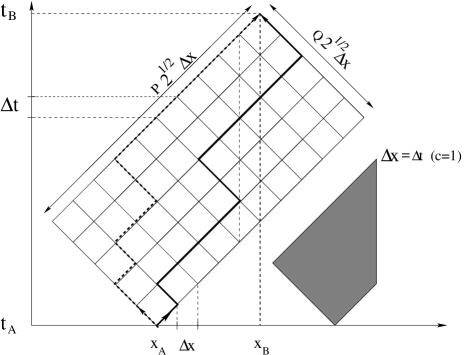
Figure 1: Checkerboard grid with $\Delta x=\Delta t$ in the $x-t$ plane $(c=1)$. Two paths with five corners, the last of which is compulsary, are shown. The solid-line path with $\alpha=+$ and $\beta=-$ does not contribute to the first-arrival propagator $K^{(1)}(x_{B},t_{B};x_{A},t_{A})$ while the dashed-line path with $\alpha=-$ and $\beta=+$ does contribute. The restricted domain for evaluation of the first-arrival propagator is bounded on the right by the vertical dotted line; its shape is shown in grey.

To begin, suppose that the spatial interval of interest is divided into $M$ pieces each of length $\Delta x=x_{BA}/M$, assuming $x_{B}>x_{A}$. Suppose further that a particular path of $N$ time-steps consists of $P$ spatial steps of length $\Delta x$ to the right and $Q$ to the left so that $N=P+Q$ and $M=P-Q$. The resulting space-time grid of path segments available to the particle is illustrated in Fig. 1. Denote by $K_{\beta\alpha}^{(1)}(B;A)$ the component of the propagator (9) associated with first arrivals at $X=x_{B}$ at time $T=t_{B}$. It is constructed from only those paths that reach $x_{B}$ for the first time at time $t_{B}$. To compute $K_{\beta\alpha}^{(1)}$ we have to count the number of $\beta\alpha$ paths with $R$ noncompulsary reversals for the restricted space-time grid shown in Fig. 1. For simplicity it is assumed that the initial wave function $\Psi(x,t_{A}=0)$ is sufficiently well localized to the left of $x_{B}=X$ that $K_{++}^{(1)}(B;A)$ and $K_{+-}^{(1)}(B;A)$ are the only components of the first-arrival propagator that need to be considered. For $x_{A}<x_{B}$ the components $K_{-+}(B;A)$ and $K_{--}(B;A)$ of course have contributions only from multiple-arrival paths.

III.1 Counting the number of first arrival paths with $R$ corners

Computation of $\Phi_{\beta\alpha}^{(1)}(R)$ involves counting the number of restricted $\beta\alpha$ paths with a given number of corners in a lattice. A path in the lattice of Fig. 2 – obtained from Fig. 1 by clockwise rotation through $45^{o}$ and rescaling by a factor of $(2^{1/2}\Delta x)^{-1}$ – is built up of $(1,0)=\;\rightarrow$ and $(0,1)=\;\uparrow$ motions. There are no $\leftarrow$ and $\downarrow$ motions because the paths of Fig. 1 move only forward in time. Denote by a $l$-corner a point on the path that is reached by a $\rightarrow$ step and is left by a $\uparrow$ step and by a $r$-corner a point that is reached by a $\uparrow$ step and left by a $\rightarrow$ step. Denote by $R_{l}$ the number of corners of type $l$ and by $R_{r}$ the number of corners of type $r$ in a given path. Any path in the $u-v$ lattice with given initial and final points $(u_{A},v_{A})$ and $(u_{B},v_{B})$ can be completely specified by either the coordinates of its $l$ corners or by the coordinates of its $r$ corners. Both specifications are needed in the following derivation of the first-arrival propagator.

First, consider the counting problem without any $\beta\alpha$ or first-arrival restrictions on the paths and including compulsary as well as noncompulsary corners. In this simple case, enumeration of the number of paths in a lattice with a given number of $l$- or $r$-corners is solved in the following manner kra . To count the number of paths with $R_{l}$ $l$-corners one builds two vectors ${\bf{u}}$ and ${\bf{v}}$ that contain the integer $u$ and $v$-coordinates of the $R_{l}$ corners of such a path:

$${\bf{u}}=(u_{1},u_{2},\cdots,u_{R_{l}})$$ (14)

$${\bf{v}}=(v_{1},v_{2},\cdots,v_{R_{l}}).$$ (15)

These coordinates satisify the inequalities

$$u_{A}+1\leq u_{1}<u_{2}\cdots<u_{R_{l}}\leq u_{B}$$ (16)

$$v_{A}\leq v_{1}<v_{2}\cdots<v_{R_{l}}\leq v_{B}-1,$$ (17)

where the sequences are strictly ordered. Denote by $\Phi_{l}^{wr}(R_{l})$ the number of paths with $R_{l}$ $l$-corners, where the label $"wr"$ is a reminder that the paths are without restriction. This number may be evaluated by observing that there are $u_{B}-u_{A}$ integers from which to choose the $u$-coordinates and $v_{B}-v_{A}$ from which to choose the $v$-coordinates. The required number is then

$$\Phi_{l}^{wr}(R_{l})=\pmatrix{u_{B}-u_{A}\cr R_{l}}\pmatrix{v_{B}-v_{A}\cr R_{l}}.$$ (18)

Similarly, one obtains

$$\Phi_{r}^{wr}(R_{r})=\pmatrix{u_{B}-u_{A}\cr R_{r}}\pmatrix{v_{B}-v_{A}\cr R_{r}}.$$ (19)

Now consider only those paths which do not cross (touching is allowed for the moment) $x=x_{B}$ before $t=t_{B}$. When considering such restricted paths in the $u-v$ lattice (see Fig. 3) it is convenient to choose the bottom-right corner of the accessible region as the origin of the $u-v$ coordinate system so that the region below the diagonal $u=v$ is out-of-bounds.

First consider the case in which the paths are specified by the coordinates of their $l$-corners. This case is the easier of the two because $l$-corners are diagnostic, i.e. a necessary and sufficient condition for a restricted path is that none of its $l$-corners be on the forbidden $u>v$ side of the diagonal. It is thus required to calculate the number of paths with $R_{l}$ $l$-corners from $(u_{A},v_{A})$ to $(u_{B},v_{B})$ with $u_{A}=a$, $v_{A}=0$ and $u_{B}=v_{B}=b$, say, such that $v_{i}\geq u_{i}$ for all $i$. This number, $\Phi_{l}(R_{l};BA)$, is the number (18) minus the number of paths with $R_{l}$ $l$-corners such that $u_{i}>v_{i}$ for at least one $i$. To calculate the latter number, take $k$ to be the largest integer such that $u_{k}>v_{k}$ and build from (16) the following sequences

$$u_{A}+1 = a+1\leq u_{1}<u_{2}\cdots<u_{k-1}<v_{k+1}\cdots<v_{R_{l}}\leq v_{B}-1\;=\;b-1$$ (20)

$$v_{A} = 0\leq v_{1}<v_{2}\cdots<v_{k}<u_{k}<u_{k+1}\cdots<u_{R_{l}}\leq u_{B}\;=\;b\;.$$ (21)

The sequences are ordered (as can be checked, see kra ) and there is a one-to-one correspondence between the double sequences (16) and the double sequences (20). The number of all the double sequences (20) is

$$\pmatrix{b-a-1\cr R_{l}-1}\pmatrix{b+1\cr R_{l}+1},$$ (22)

and therefore $\Phi_{l}(R_{l};BA)$ is given by

$$\Phi_{l}(R_{l};BA)=\pmatrix{b-a\cr R_{l}}\pmatrix{b\cr R_{l}}-\pmatrix{b-a-1\cr R_{l}-1}\pmatrix{b+1\cr R_{l}+1}.$$ (23)

Now consider, the computation of the corresponding number of restricted paths from $(a,0)$ to $(b,b)$ with $R_{r}$ $r$-corners, i.e. $\Phi_{r}(R_{r};BA)$. A necessary condition for such a path is, of course, that all of its $R_{r}$ $r$-corners be on the allowed $v>u$ side of the diagonal. However, this is not a sufficient condition because it is possible for the $l$-corner between two consecutive such $r$-corners to be on the forbidden side of the diagonal. An additional complication is that the first $l$-corner might precede the first $r$-corner and/or the last $l$-corner might follow the last $r$-corner. A simple way to include such $l$-corners in the analysis is to add the end-points $(a,0)\equiv(u_{0},v_{0})$ and $(b,b)\equiv(u_{R_{r}+1},v_{R_{r}+1})$ to the set of $R_{r}$ $r$-corners to obtain the set of $R_{r}+2$ points $\{(u_{0},v_{0}),(u_{1},v_{1}),...,(u_{R_{r}},v_{R_{r}}),(u_{R_{r}+1},v_{R_{r}+1})\}$. Now, for $1\leq i\leq R_{r}-1$, $(u_{i+1},v_{i})$ is the (diagnostic) $l$-corner between the consecutive r-corners $(u_{i},v_{i})$ and $(u_{i+1},v_{i+1})$. Hence, $\Phi_{r}(R_{r};BA)$ is the number (19) minus the number of paths with $R_{r}$ $r$-corners such that $u_{i+1}>v_{i}$ for at least one $i$, with $0\leq i\leq R_{r}$ to allow for paths for which the first and/or last corner is an $l$-corner. To calculate the latter number, take $k$ to be the smallest integer such that $u_{k+1}>v_{k}$ and construct the sequences

$$a=u_{0}\leq u_{1}<u_{2}<...<u_{k}<v_{k+1}<...<v_{R_{r}}\leq v_{R_{r}+1}=b$$ (24)

$$1=v_{0}+1\leq v_{1}<v_{2}<...<v_{k}<u_{k+1}<...<u_{R_{r}}\leq u_{R_{r}+1}-1=b-1\;.$$ (25)

The total number of these double sequences is

$$\pmatrix{b-a+1\cr R_{r}}\pmatrix{b-1\cr R_{r}}\;,$$ (26)

and therefore $\Phi_{r}(R_{r};BA)$ is given by

$$\Phi_{r}(R_{r};BA)=\pmatrix{b-a\cr R_{r}}\pmatrix{b\cr R_{r}}-\pmatrix{b-a+1\cr R_{r}}\pmatrix{b-1\cr R_{r}}\;.$$ (27)

Finally, consider the desired $\beta\alpha$ first-arrival paths, which are not allowed to touch $x=x_{B}$ before $t=t_{B}$. The various notations $A$, $(x_{A},t_{A})$ and $(u_{A},v_{A})2^{1/2}\Delta x$ are reserved for the first point of a checkerboard path and $B$, $(x_{B},t_{B})$ and $(u_{B},v_{B})2^{1/2}\Delta x$ for the last point. Denote by $A_{\alpha}$, $(x_{A}+\alpha\Delta x,t_{A}+\Delta t)$ and $(a_{\alpha},0)2^{1/2}\Delta x$ the point on a $\beta\alpha$ path at time $t=t_{A}+\Delta t$ and by $B_{\beta}$, $(x_{B}-\beta\Delta x,t_{B}-\Delta t)$, $(b_{\beta},b_{\beta})2^{1/2}\Delta x$ the point at time $t=t_{B}-\Delta t$.

It is important to note that those paths which may touch but do not cross the diagonal $u=v$, extending from $(0,0)$ to $(b_{\beta},b_{\beta})$, do not touch $x=x_{B}$ before $t=t_{B}$ and hence are first-arrival paths. Hence, the above expressions for $\Phi_{l}(R_{l};BA)$ and $\Phi_{r}(R_{r};BA)$ with $A$, $B$, $a$ and $b$ replaced by $A_{\alpha}$, $B_{\beta}$, $a_{\alpha}$ and $b_{\beta}$, respectively, can be used to evaluate $\Phi^{(1)}_{\beta\alpha}$ and hence $K^{(1)}_{\beta\alpha}$. It is only necessary, for a given choice of $\alpha$ and $\beta$, to determine $a_{\alpha}$, $b_{\beta}$ and the relation between $R$ and $R_{l}$ or $R_{r}$, keeping in mind that $R$ includes only noncompulsary corners.

For $\beta\alpha\>=\>++$ it is clear from Fig. 4 that $(b_{+},b_{+})=(Q,Q)$, $(u_{B},v_{B})=(Q+1,Q)$, $(u_{A},v_{A})=(Q+1-P,0)$ and $(a_{+},0)=(Q+2-P,0)$. Then a little thought leads to the conclusion that the number $\Phi_{++}^{(1)}(R)$ is equal to $\Phi_{r}(R_{r};B_{+}A_{+})$ with the identification $R=2R_{r}-1$. Hence, upon replacing $a$ by $a_{+}=Q+2-P$, $b$ by $b_{+}=Q$, and $R_{r}$ by $(R+1)/2$ in (27), it follows that

$$\Phi_{++}^{(1)}(R) = \pmatrix{P-2\cr(R+1)/2}\pmatrix{Q\cr(R+1)/2}-\pmatrix{P-1\cr(R+1)/2}\pmatrix{Q-1\cr(R+1)/2}$$ (28)

$$= \pmatrix{P-1\cr(R+1)/2}\pmatrix{Q-1\cr(R-1)/2}-\pmatrix{P-2\cr(R-1)/2}\pmatrix{Q\cr(R+1)/2},$$ (30)

where the identity $\pmatrix{n-1\cr k}=\pmatrix{n\cr k}-\pmatrix{n-1\cr k-1}$ has been used.

For $\beta\alpha\>=\>+-$ it is clear from Fig. 5 that $(b_{+},b_{+})=(Q-1,Q-1)$, $(u_{B},v_{B})=(Q,Q-1)$, $(a_{-},0)=(Q-P,0)$, $(u_{A},v_{A})=(Q-P,-1)$ and $\Phi_{+-}^{(1)}(R)$ is equal to $\Phi_{l}(R_{l};B_{+}A_{-})$ with $R=2R_{l}$. Hence, upon replacing $a$ by $a_{-}=Q-P$, $b$ by $b_{+}=Q-1$ and $R_{l}$ by $R/2$ in (23), it follows that

$$\Phi_{+-}^{(1)}(R)=\pmatrix{P-1\cr R/2}\pmatrix{Q-1\cr R/2}-\pmatrix{P-2\cr(R-2)/2}\pmatrix{Q\cr(R+2)/2},$$ (31)

with $\Phi_{+-}^{(1)}(1)=1$.

III.2 Evaluation of the propagators

The first-arrival-time propagators are expressed as

$$K_{++}^{(1)}(B;A)=\frac{i}{2\lambda_{c}}\>\lim_{N\to\infty}\sum_{odd\;R\geq 1}\Phi_{++}^{(1)}(R)(im\Delta t)^{R}$$ (32)

$$K_{+-}^{(1)}(B;A)=\frac{i}{2\lambda_{c}}\>\lim_{N\to\infty}\sum_{even\;R\geq 0}\Phi_{+-}^{(1)}(R)(im\Delta t)^{R}.$$ (33)

III.3 The case of $K_{++}^{(1)}$

In this case we have from (32) and using the approximation $\pmatrix{n\cr m}\approx n^{m}/m!$, that becomes exact as $n\to\infty$,

$$K_{++}^{(1)}(B;A) = \frac{i}{2\lambda_{c}}\lim_{N\to\infty}\sum_{odd\;R\>\geq 1}(im\Delta t)^{R}\Bigg{(}\frac{P^{(R+1)/2}}{[(R+1)/2]!}\frac{Q^{(R-1)/2}}{[(R-1)/2]!}-\frac{P^{(R-1)/2}}{[(R-1)/2]!}\frac{Q^{(R+1)/2}}{[(R+1)/2]!}\Bigg{)}$$ (34)

$$= \frac{i}{2\lambda_{c}}\lim_{N\to\infty}\sum_{odd\;R\geq 1}(im\Delta t)^{R}(P-Q)\frac{(PQ)^{(R-1)/2}}{[(R+1)/2]!([(R-1)/2]!}.$$ (35)

This expression may be transformed to

$$K_{++}^{(1)}(B;A) = i\frac{x_{BA}}{\lambda_{c}l_{BA}}\>\lim_{N\to\infty}\sum_{odd\>R\geq 1}\biggl{(}\frac{il_{BA}}{2\lambda_{c}}\biggr{)}^{R}\frac{1}{[(R+1)/2]![(R-1)/2]!}$$ (36)

$$= -\frac{x_{BA}}{\lambda_{c}l_{BA}}\>\cdot\>\frac{l_{BA}}{2\lambda_{c}}\sum_{k=0}^{\infty}(-)^{k}\biggl{(}\frac{l_{BA}}{2\lambda_{c}}\biggr{)}^{2k}\frac{1}{k!(k+1)!}\;.$$ (37)

In the last line $R$ has been replaced by $2k+1$ and the limit $N\rightarrow\infty$ taken. Comparison with the power series representation of the Bessel function,

$$J_{n}(z)=(\frac{z}{2})^{n}\sum_{k=0}^{\infty}\frac{(-)^{k}}{k!(k+n)!}(\frac{z}{2})^{2k},$$ (38)

immediately gives

$$K_{++}^{(1)}(B;A)=-\frac{x_{BA}}{\lambda_{c}l_{BA}}J_{1}\biggl{(}\frac{l_{BA}}{\lambda_{c}}\biggr{)}\;.$$ (39)

III.4 The case of $K_{+-}^{(1)}$

In this case we start with the expression

$$K_{+-}^{(1)}(B;A)=\frac{i}{2\lambda_{c}}\lim_{N\to\infty}\sum_{even\>R\>\geq 0}(im\Delta t)^{R}\Biggl{(}\frac{P^{R/2}}{(R/2)!}\frac{Q^{R/2}}{(R/2)!}-\frac{P^{(R-2)/2}}{[(R-2)/2]!}\frac{Q^{(R+2)/2}}{[(R+2)/2]!}\Biggr{)}.$$ (40)

Steps analogous to those above lead to

$$K_{+-}^{(1)}(B;A)=\frac{i}{2\lambda_{c}}\;\Biggl{[}J_{0}\biggl{(}\frac{l_{BA}}{\lambda_{c}}\biggr{)}+\frac{c-v_{BA}}{c+v_{BA}}\;J_{2}\biggl{(}\frac{l_{BA}}{\lambda_{c}}\biggr{)}\Biggr{]}\>.$$ (41)

An interesting equality emerges from the above results, namely

$$K_{++}(B;A)\;-\;K_{--}(B;A)=K_{++}^{(1)}(B;A).$$ (42)

In fact all paths contributing to the $K_{--}(B;A)$ component of the propagator touch the line $x=x_{B}$ at least twice and therefore this set of paths is complementary to the one contributing to $K_{++}^{(1)}(B;A)$ in the limit of $N\to\infty$.

Finally,

$$K_{++}^{(2,3,\cdots)}(B;A)=K_{++}(B;A)-K_{++}^{(1)}(B;A)=K_{--}(B;A) = \frac{x_{BA}-ct_{BA}}{2\lambda_{c}l_{BA}}\;J_{1}\biggl{(}\frac{l_{BA}}{\lambda_{c}}\biggr{)}$$ (43)

$$K_{+-}^{(2,3,\cdots)}(B;A)=K_{+-}(B;A)-K_{+-}^{(1)}(B;A) = -\>\frac{i}{2\lambda_{c}}\;\frac{c-v_{BA}}{c+v_{BA}}\;J_{2}\biggl{(}\frac{l_{BA}}{\lambda_{c}}\biggr{)}.$$ (44)

IV Interference between first and later arrivals

The decomposition $K_{\beta\alpha}(B;A)\>=\>K_{\beta\alpha}^{(1)}(B;A)\>+\>K_{\beta\alpha}^{(2,3,...)}(B;A)$ according to first and later (second, third, etc.) arrivals of a particle at $x_{B}$ at $t_{B}$ leads immediately to the corresponding decomposition $\Psi_{\beta}(x_{B},t_{B})\>=\>\Psi_{\beta}^{(1)}(x_{B},t_{B})\>+\>\Psi_{\beta}^{(2,3,...)}(x_{B},t_{B})$ for the $\beta=\pm$ components of the wave function $\Psi(x_{B},t_{B})$. Substitution of the latter expression, with $t_{A}=0$, $x_{B}=X$ and $t_{B}=T$, into the result (13) for the arrival-time distribution gives

$$\Pi(T;X)\>=\>\Pi^{(1)}(T;X)\>+\>\Pi^{(2,3,...)}(T;X)\>+\>\Pi^{(1\>\times\>2,3,...)}(T;X)\;.$$ (45)

For the special case considered here in which the initial probability density $\rho(x_{A},0)$ is negligible for $x_{A}\geq X$,

$$\Pi^{(1)}(T;X)=C\biggl{|}\int_{-\infty}^{X}\!dx_{A}\bigl{[}K^{(1)}_{++}(X,T;x_{A},0)\Psi_{+}(x_{A},0)+K^{(1)}_{+-}(X,T;x_{A},0)\Psi_{-}(x_{A},0)\bigr{]}\biggr{|}^{2}$$ (46)

is the contribution of first arrivals,

$$\Pi^{(2,3,...)}(T;X)\!\! = \!\!C\biggl{|}\int_{-\infty}^{X}\!dx_{A}\bigl{[}K^{(2,3,...)}_{++}(X,T;x_{A},0)\Psi_{+}(x_{A},0)+K^{(2,3,...)}_{+-}(X,T;x_{A},0)\Psi_{-}(x_{A},0)\bigr{]}\biggr{|}^{2}$$ (47)

$$+ \!\!C\biggl{|}\int_{-\infty}^{X}\!dx_{A}\bigl{[}K^{(2,3,...)}_{-+}(X,T;x_{A},0)\Psi_{+}(x_{A},0)+K^{(2,3,...)}_{--}(X,T;x_{A},0)\Psi_{-}(x_{A},0)\bigr{]}\biggr{|}^{2}$$ (48)

is the contribution of later-arrivals and

$$\Pi^{(1\>\times\>2,3,...)}(T;X)\! = \!2C\>\Re\biggl{\{}\int_{-\infty}^{X}\!dx_{A}\bigl{[}K^{(1)}_{++}(X,T;x_{A},0)\Psi_{+}(x_{A},0)+K^{(1)}_{+-}(X,T;x_{A},0)\Psi_{-}(x_{A},0)\bigr{]}^{*}$$ (50)

$$\times \!\int_{-\infty}^{X}\!dx_{A}\bigl{[}K^{(2,3,...)}_{++}(X,T;x_{A},0)\Psi_{+}(x_{A},0)+K^{(2.3,...)}_{+-}(X,T;x_{A},0)\Psi_{-}(x_{A},0)\bigr{]}\biggr{\}}$$ (51)

is the contribution due to interference between first and later arrivals. ($C$ is the normalization factor appearing in (13)). Of particular interest here is the magnitude of the interference contribution relative to the first-arrival contribution in the regime $v_{BA}<<c$.

First, however, briefly consider the regime in which $v_{BA}$ is so close to $c$ that the correlation distance $\lambda_{c}[1-(v_{BA}/c)^{2}]^{-1/2}$ for reversal of direction is sufficiently large that for a typical checkerboard path there is insufficient time for more than one arrival at $x_{B}$. To be more quantitative, assume that the initial amplitude $\Psi_{-}(x_{A},t_{A})$ of the $-c$ velocity eigenstate is completely negligible with respect to the initial amplitude $\Psi_{+}(x_{A},t_{A})$ of the $+c$ eigenstate so that one need consider only $K_{++}(B;A)$ and $K_{-+}(B;A)$. Also, for $(x_{B},t_{B})=(X,T)$ and $(x_{A},t_{A})=(x_{A},0)$ assume that $x_{BA}=X-x_{A}$ is very close to $ct_{BA}=cT$ for those values of $T$ for which $\Pi(T;X)$ is nonnegligible and for those values of $x_{A}$ for which $\rho(x_{A},0)$ is nonnegligible. In this regime, $K_{++}^{(1)}(B;A)/K_{++}(B;A)\approx 1-\delta/2$ and $K_{++}^{(2,3,...)}(B;A)/K_{++}(B;A)\approx\delta/2$ where $v_{BA}\equiv(1-\delta)c$ with $\delta<<1$. In addition, $|K_{-+}(B;A)/K_{++}(B;A)|\approx(l_{BA}/2ct_{BA})J_{0}(l_{BA}/\lambda_{c})/J_{1}(l_{BA}/\lambda_{c})$ with $l_{BA}\approx(2\delta)^{1/2}ct_{BA}$. If $\delta$ is sufficiently small that $l_{BA}<<\lambda_{c}$ then, using the leading term in (38) for $n=0$ and for $n=1$, $|K_{-+}(B;A)/K_{++}(B;A)|\approx\lambda_{c}/x_{BA}=\lambda_{c}/(X-x_{A})$ which is typically very much less than $1$ for an initial wave packet $\Psi(x_{A},0)$ that is well-localized away from $x=X$. Hence, at least to the extent that the concepts of single-particle probability and probability current densities are still meaningful in the regime in which $v_{BA}$ is very close to $c$, the interference term is very small and $\Pi(T;X)=\Pi^{(1)}(T;X)$ to a good approximation. Strictly speaking, however, for the special case under consideration the first-arrival-time distribution is well-defined only in the limit $v_{BA}\rightarrow c$.

Now, consider the nonrelativistic regime. With the definitions $\Psi_{\pm}(x,t)\equiv\phi_{\pm}(x,t)\exp(-imc^{2}t/\hbar)$, $\phi(x,t)\equiv\phi_{+}(x,t)+\phi_{-}(x,t)$ and $\Delta\phi(x,t)\equiv\phi_{+}(x,t)-\phi_{-}(x,t)$, the $1$ + $1$ dimensional free-electron Dirac equation (1) can be written

$$i\hbar\>\partial\phi(x,t)/\partial t\> = \>-i\hbar c\>\partial\Delta\phi(x,t)/\partial x-2mc^{2}\phi(x,t)\;,$$ (53)

$$i\hbar\>\partial\Delta\phi(x,t)/\partial t\> = \>-i\hbar c\>\partial\phi(x,t)/\partial x\;.$$ (54)

If $i\hbar\partial\phi/\partial t$ is negligible with respect to $2mc^{2}\phi$ (with $c$ fixed at its actual value, not set equal to infinity) then $\phi$ can be replaced by $-(i\hbar/2mc)\partial\Delta\phi/\partial x$ in the second equation of (53) to obtain the Schrödinger equation $i\hbar\partial\Delta\phi(x,t)/\partial t=-(\hbar^{2}/2m)\partial^{2}\Delta\phi(x,t)/\partial x^{\;2}$. If one further assumes that $|\Delta\phi(x,t)|^{2}>>|\phi(x,t)|^{2}$ and identifies $2^{-1/2}\Delta\phi(x,t)$ with the Schrödinger wave function $\psi_{S}(x,t)$ then the expressions (7) and (8) immediately lead to the desired nonrelativistic expressions, $\rho_{S}(x,t)=|\psi_{S}(x,t)|^{2}$ and $J_{S}(x,t)=(\hbar/m)\Im[\psi_{S}^{*}(x,t)\partial\psi_{S}(x,t)/\partial x]$ respectively, for the nonrelativistic probability and probability current densities. Consistent with these considerations is the following simple choice of initial $(t=0)$ wave function $\Psi(x_{A},0)$ for the nonrelativistic regime: $\Psi_{+}(x_{A},0)=-g\Psi_{0}(x_{A})$ and $\Psi_{-}(x_{A},0)=(1-g^{2})^{1/2}\Psi_{0}(x_{A})$ where $g$ is a real constant very close to $2^{-1/2}$ (see below) and $\Psi_{0}(x)=(2\pi)^{-1/4}(\Delta x)^{-1/2}\exp[-(2\Delta x)^{-2}(x-x_{0})^{2}+ik_{0}x]$ is a minimum-uncertainty-product gaussian with initial centroid $x_{0}$, initial variance $\Delta x$, mean wave vector $k_{0}$ and variance $\Delta k=1/2\Delta x$. In the numerical calculations presented below the constant $g$ is chosen so that the characteristic velocity $v(x_{A},0)\equiv J(x_{A},0)/\rho(x_{A},0)=(2g^{2}-1)c\equiv v$ (independent of $x_{A}$) is equal to $v_{0}\equiv\hbar k_{0}/m$ with $v_{0}<<c$.

Now, from (10), (11) and (39) it immediately follows that

$$K_{++}^{(1)}(B;A)/K_{++/--}(B;A)\>=\>2v_{BA}/(c\pm v_{BA})\>\approx\>2v_{BA}/c$$ (55)

and from (12) and (41) it follows that

$$\frac{K_{+-}^{(1)}(B;A)}{K_{+-/-+}(B;A)}\> = \>\frac{J_{0}(l_{BA}/\lambda_{c})+[(c-v_{BA})/(c+v_{BA})]J_{2}(l_{BA}/\lambda_{c})}{J_{0}(l_{BA}/\lambda_{c})}$$ (56)

$$\approx \>\frac{J_{0}(l_{BA}/\lambda_{c})+J_{2}(l_{BA}/\lambda_{c})-(2v_{BA}/c)J_{2}(l_{BA}/\lambda_{c})}{J_{0}(l_{BA}/\lambda_{c})}.$$ (57)

In the regime $v_{BA}/c<<1$ under consideration, $l_{BA}/\lambda_{c}\approx ct_{BA}/\lambda_{c}=(c/v_{BA})(x_{BA}/\lambda_{c})>>x_{BA}/\lambda_{c}>>1$. Using the leading two terms in Hankel’s asymptotic expansions AbSteg of $J_{0}(z)$ and $J_{2}(z)$ for large argument $z$, i.e.

$$J_{0}(z)\> \approx \>\biggl{(}\frac{2}{\pi z}\biggr{)}^{1/2}\biggl{[}\cos\biggl{(}z-\;\frac{\pi}{4}\biggr{)}\>+\>\frac{1}{8z}\sin\biggl{(}z-\frac{\pi}{4}\;\biggr{)}\biggr{]}\;\;(|z|>>1)$$ (58)

$$J_{2}(z)\> \approx \>\biggl{(}\frac{2}{\pi z}\biggr{)}^{1/2}\biggl{[}\cos\biggl{(}z-\frac{5\pi}{4}\biggr{)}-\frac{15}{8z}\sin\biggl{(}z-\frac{5\pi}{4}\biggr{)}\biggr{]}\>\>(|z|>>1)\;,$$ (59)

gives

$$\frac{K_{+-}^{(1)}(B;A)}{K_{+-/-+}(B;A)}\;\approx\;2\;\biggl{(}\frac{v_{BA}}{c}\biggr{)}\;\frac{\cos\biggl{(}\frac{l_{BA}}{\lambda_{c}}\>-\>\frac{\pi}{4}\biggr{)}\>+\>\frac{\lambda_{c}}{16x_{BA}}\>\sin\biggl{(}\frac{l_{BA}}{\lambda_{c}}\>-\>\frac{\pi}{4}\biggr{)}}{\cos\biggl{(}\frac{l_{BA}}{\lambda_{c}}\>-\>\frac{\pi}{4}\biggr{)}\>+\>\frac{\lambda_{c}}{8l_{BA}}\sin\biggl{(}\frac{l_{BA}}{\lambda_{c}}\>-\>\frac{\pi}{4}\biggr{)}}\>.$$ (60)

For $l_{BA}/\lambda_{c}=(4n+3)\pi/4$ with $n$ an integer, the right-hand-side of (60) is $1$. However, in a well-designed arrival-time experiment for the wave function under discussion one would arrange that $(X-x_{0})>>\Delta x$ so that $\rho(x_{A},0)$ is completely negligible for $x_{A}\geq X$ and also that $\Delta x>>\lambda_{c}$ so that there is negligible probability of generating particle-antiparticle pairs. Hence, $\lambda_{c}/x_{BA}$ would be extremely small over the important range of $x_{BA}$. Hence, the set of $x_{BA}$ values where the right-hand-side of (60) is not close to $2v_{BA}/c$ is of small measure and can be ignored when considering integrals over $x_{A}$, provided that $v_{BA}/c$ is not itself extremely small (a rough estimate requires that $v_{BA}/c\;>>\;\lambda_{c}/16\pi x_{BA}$).

Taking into account that $-\Psi_{-}(x_{A},0)\approx\Psi_{+}(x_{A},0)$ for $|v(x_{A},0)|<<c$ and that the terms involving $K_{--}^{(1)}$ and $K_{-+}^{(1)}$ are negligible when $|X-x_{0}|>>\Delta x$ then leads directly to the estimates

$$\Pi^{(1)}(T;X)\;\approx\;(1/2)(2v/c)^{2}\;\Pi(T;X)\;=\;2(v/c)^{2}\;\Pi(T;X)\;,$$ (61)

$$\Pi^{(1\times 2,3,...)}(T;X)\;\approx\;2(1/2)(2v/c)\;\Pi(T;X)\;=\;2(v/c)\;\Pi(T;X)\;$$ (62)

for the gaussian wave function under consideration. It should be noted that $v_{BA}=(X-x_{A})/T$ has been approximated by $v$ which is consistent with $(X-x_{0})>>\Delta x$ in the absence of significant wave packet spreading. Fig. 6 and Fig. 7 show results for $\Pi(T;0)$, $\Pi^{(1)}(T;0)/2(v/c)^{2}$ and $\Pi^{(1\times 2,3,...)}(T;0)/2(v/c)$ obtained by numerical evaluation of (46) to (50) for gaussian wave packets with $\Delta k/k_{0}=0.02$ and $0.2$ respectively. In the former case the above estimates are excellent approximations; in the latter case, even though wave packet spreading is more important, the estimates still provide good approximations for the very large differences in overall scale between the three quantities.

V Concluding Remarks

In summing up, it is interesting to make a qualitative comparison of the results of the Feynman path and Bohm trajectory approaches for investigating arrival times for Dirac electrons.

In Bohmian mechanics BH ; HOLLAND ; CFG an electron is postulated to be an actually existing point-like particle and an accompanying wave which guides its motion. For a Dirac electron in the presence of a potential $V(\vec{r},t)$, the time-evolution of the guiding wave $\Psi(\vec{r},t)$ is described by the $3$D Dirac equation and the trajectory of the point-like particle is determined by the equation-of-motion $d\vec{r}(t)/dt=[\vec{J}(\vec{r},t)/\rho(\vec{r},t)]|_{\vec{r}=\vec{r}(t)}$. It is further postulated that, for an ensemble of electrons all prepared in the same initial state $\Psi(\vec{r},0)$, the probability of such a particle having initial position $\vec{r}^{\>(0)}\equiv\vec{r}(t=0)$ is given by $\rho(\vec{r}^{\>(0)},0)$. The various properties stated below for the intrinsic arrival times of the point-like particles of Bohm’s theory follow readily from the fact that, for a given initial wave function, trajectories with different starting points $\vec{r}^{\>(0)}$ never intersect or even touch each other TQM .

Now, the expression for the intrinsic $1$D arrival-time distribution obtained with either approach can be cast in the same form as in classical mechanics, namely

$$\Pi(T;X)=\Pi_{+}(T;X)+\Pi_{-}(T;X)\;\;;\;\;\Pi_{\pm}(T;X)\equiv\pm J_{\pm}(X,T)\bigg{/}\int_{0}^{T_{max}}dt[J_{+}(X,t)-J_{-}(X,t)]\;,$$ (63)

where $J_{+}$ and $J_{-}$, respectively, are the right-going and left-going components of the probability current density $J$. The decomposition $J\>=\>J_{+}\;+\;J_{-}$ is not uniquely defined. The decomposition associated with the fictitious particles of the checkerboard path approach, which move only at the speed of light $c$, is $J_{\pm}=\pm\>c\>|\Psi_{\pm}|^{2}$ while that associated with the (assumed) actual particles of the Bohm trajectory approach, each of which moves at a variable speed that cannot exceed $c$, is $J_{\pm}\>=\>J\Theta[\pm J]$ where $\Theta$ is the unit step-function. The former decomposition leads to an arrival-time distribution $\Pi(T;X)$ proportional to the probability density $\rho(X,T)$ while the latter leads to one proportional to the absolute value of the probability current density, i.e $|J(X,T)|$. Moreover, unless one or other (or both) of the two components of $\Psi(X,t)$ is zero for $T_{1}\leq t\leq T_{2}$, there are more arrivals – many more if $T_{2}-T_{1}$ is much larger than the Jacobson-Schulman correlation time – of the fictitious particles at $X$ during that time interval than there are of the supposed actual particles of Bohm’s theory.

Given the probability current density $J(x,t)$ and using the non-crossing property of Bohm trajectories it is straightforward to decompose the intrinsic arrival-time distribution into contributions from first arrivals, from second arrivals, etc. with no interference terms between different orders of arrival ROSS . In marked contrast to this, the decomposition based on Feynman checkerboard paths in general contains a nonzero interference term between first and later (i.e., second, third, …) arrivals so that from the calculation one cannot extract a well-defined intrinsic first-arrival-time distribution. In the nonrelativistic regime this interference term can be very large compared to the first-arrival term. Because of this and the extremely small correlation length for reversal of direction ($\approx\lambda_{c}$ which is only about $10^{-3}$ of the diameter of an atom!), suppression of the interference term by decoherence JJH within a time interval much less than $\lambda_{c}/c$ in duration immediately following the instant of first arrival would be very difficult, if not impossible, in a practical arrival-time measurement. Unless this can be achieved, assuming that the first-arrival times of the fictitious particles of the checkerboard model are directly relevant to the arrival times measured in a time-of-flight experiment on actual electrons is not justified.

Figure 2: Example of an unrestricted path that would not be allowed once first-arrival restrictions are introduced. The $u$ and $v$ sequences corresponding to the three $l$-corners and two $r$-corners of the path are indicated.

Figure 3: A restricted path from $(u_{A},v_{A})=(a,0)$ to $(u_{B},v_{B})=(b,b)$ which has two $l$-corners and three $r$-corners.

Figure 4: The dashed line demarcates the grid to be considered in the enumeration problem related to $K_{++}^{(1)}$.

Figure 5: The dashed line demarcates the grid to be considered in the enumeration problem related to $K_{+-}^{(1)}$.

Figure 6: Arrival-time distribution $\Pi(T;0)$ (solid curve), scaled first-arrival contribution $\Pi^{(1)}(T;0)/2(v/c)^{2}$ (dotted line) and scaled interference contribution $\Pi^{(1\times 2,3,...)}(T;0)/2(v/c)$ (dashed line) for the initial gaussian wave function described in the text. $k_{0}=1.00$ Å^-1, $\Delta k=0.02$ Å^-1 and $x_{0}=-6\Delta x$ with $\Delta x=1/2\Delta k$; $v/c=v_{0}/c=3.862\times 10^{-3}$; $t_{0}\>\equiv\>|x_{0}|/v_{0}\>=\>1.296\times 10^{-14}$ sec and $T_{max}=2t_{0}$.

Figure 7: Arrival-time distribution $\Pi(T;0)$ (solid line), scaled first-arrival contribution $\Pi^{(1)}(T;0)/2(v/c)^{2}$ (dotted line) and scaled interference contribution $\Pi^{(1\times 2,3,...)}(T,0)/2(v/c)$ (dashed line) for the initial gaussian wave function described in the text. $k_{0}=1.00$ Å^-1, $\Delta k=0.2$ Å^-1 and $x_{0}=-8\Delta x$ with $\Delta x=1/2\Delta k$; $v/c=v_{0}/c=3.862\times 10^{-3}$; $t_{0}=1.728\times 10^{-15}$ sec and $T_{max}=3t_{0}$.

References

• (1) J. G. Muga, R. Sala and J. P. Palao, Superlattices and Microstructures 23, 833 (1998).
• (2) J. G. Muga and C. R. Leavens, Phys. Rep. 338, 353 (2000).
• (3) Time in Quantum Mechanics, edited by J. G. Muga, R. Sala Mayato and I. L. Egusquiza (Springer-Verlag, Berlin, 2002).
• (4) R. P. Feynman and A. R. Hibbs, Quantum Mechanics and Path Integrals (McGraw-Hill, New York, 1965), p.34-36.
• (5) N. Yamada and S. Takagi, Prog. Theor. Phys. 85, 985 (1991).
• (6) N. Yamada and S. Takagi, Prog. Theor. Phys. 86, 599 (1991).
• (7) T. Jacobson and L. S. Schulman, J. Phys. A 17, 375 (1984).
• (8) C. R. Leavens, Phys. Lett. A 272, 160 (2000).
• (9) E. P. Wigner, in Aspects of Quantum Theory, edited by A. Salam and E. P. Wigner (Cambridge University Press, London, 1972).
• (10) B. Gaveau, T. Jacobson, M. Kac and L. S. Schulman, Phys. Rev. Lett. 53, 419 (1984).
• (11) L. S. Schulman, in Path Summation: Achievements and Goals, edited by S. Lundqvist, A. Ranfagni, V. Sa-yakanit and L. S. Schulman (World Scientific, Singapore, 1988).
• (12) C. Krattenthaler, The enumeration of lattice paths with respect to their number of turns, in “Advances in Combinatorial Methods and Applications to Probability and Statistics”, pp. 29-58, N. Balakrishnan, Brirkhäuser, Boston (1997).
• (13) M. Abramowitz and I. E. Stegum, Handbook of Mathematical Functions (National Bureau of Standards, Washington, 1970).
• (14) D. Bohm and B. Hiley, The Undivided Universe: An Ontological Interpretation of Quantum Mechanics (Routledge, London, 1993).
• (15) P. R. Holland, The Quantum Theory of Motion (Cambridge University Press, Cambridge, 1993).
• (16) J. T. Cushing, A. Fine and S. Goldstein (eds), Bohmian Mechanics and Quantum Theory: An Appraisal (Kluwer, Dordrecht, 1996).
• (17) C. R. Leavens, in Time in Quantum Mechanics, edited by J. G. Muga, R. Sala Mayato and I. L. Egusquiza (Springer, Berlin, 2002), Ch. 5.
• (18) W. R. McKinnon and C. R. Leavens, Phys. Rev. A 51, 2748 (1995); X. Oriols, F. Martín and J. Suñé, Phys. Rev. A 54, 2594 (1996).
• (19) J. J. Halliwell, in Time in Quantum Mechanics, edited by J. G. Muga, R. Sala Mayato and I. L. Egusquiza (Springer, Berlin, 2002), Ch. 6.
Refer to caption