Parameter scaling in the decoherent quantum-classical
transition for chaotic systems

Abstract

The quantum to classical transition has been shown to depend on a number of parameters. Key among these are a scale length for the action, $\hbar$, a measure of the coupling between a system and its environment, $D$, and, for chaotic systems, the classical Lyapunov exponent, $\lambda$. We propose computing a measure, reflecting the proximity of quantum and classical evolutions, as a multivariate function of $(\hbar,\lambda,D)$ and searching for transformations that collapse this hyper-surface into a function of a composite parameter $\zeta=\hbar^{\alpha}\lambda^{\beta}D^{\gamma}$. We report results for the quantum Cat Map, showing extremely accurate scaling behavior over a wide range of parameters and suggest that, in general, the technique may be effective in constructing universality classes in this transition.

The classical description of a system approximates the inherently quantum world and has significantly different predictions. The question of when quantum mechanics reduces to classical behavior is both fundamentally interesting as well as relevant to applications such as quantum computing which seek to exploit this difference. The quantum to classical transition (QCT) is now understood to be affected not only by the relative size of $\hbar$ (Planck’s constant) for a given system, but also by $D$, a measure of the coupling of the environment to the quantum system of interest, an effect termed decoherence. Further, in systems where the classical evolution is chaotic, the transition is also affected by the chaos in the system, and thus by $\lambda$, the Lyapunov exponent of the classical trajectory dynamics zp ; pb . As such, the QCT for chaotic Hamiltonians is, in general, a complicated function of multiple parameters, and is far from being fully understood.

However, the parametric dependence is as daunting as it first appears, particularly near the transition regime. Several studies point to composite parameters, indicating that the transition is not independently affected by each of the three parameters. For example, considerations ott ; doron ; zp ; koslovsky ; pb ; ap of stochastic quantum evolution or a master equation show that the parameter range for classical behavior is not simply $\hbar\ll 1$ but depends also on $D$. These and similar studies also indicate scaling relationships involving $\hbar,D,\lambda$. Other work has addressed correspondence at level of trajectories which requires a continuous extraction of information from the environment tanmoy , as opposed to tracing over these variables. However, here again, the condition for correspondence may be viewed as a composite variable where $D$ is appropriately replaced by the strength of the measurement. More recently, it has been argued that Hamiltonian systems fall into a range of universality classes with distinctly different QCTs salman , behavior manifested in the density matrix far from the transition regime.

With these as motivation, we propose that significant progress can be made by (a) computing measures which directly reflect the ‘distance’ between quantum and classical evolutions as a function of $\hbar,\lambda,\;\mbox{and}\;D$ and then (b) searching for transformations that collapse the resulting hyper-surface onto a function of a composite parameter of the form $\zeta=\hbar^{\alpha}\lambda^{\beta}D^{\gamma}$. The aims are (i) to search for this scaling, especially the coefficients $\alpha,\beta,\gamma$ fn1 ; (ii) to investigate the range of parameters and initial conditions over which the scaling holds and (iii) to study the dependence of the distance measure on $\zeta$. We can anticipate the possible outcomes: First, that $\alpha,\beta,\gamma$ are independent of the Hamiltonian. If this extremely unlikely scenario holds, we have a modified Planck’s constant governing all quantum chaotic systems, and universality classes are differentiated by differing dependences of the distance measure on $\zeta$. Second, a range of behavior for $\alpha,\beta,\gamma$ is seen, including a dependence on initial conditions, providing a classification scheme possibly correlated with the previously proposed classes. Finally, any scaling may be associated with the nature (single-scale, multi-scale) of the quantum coherence affected by the environment. This suggests a third alternative where scaling behavior exists only for limited classes of systems or limited parameter ranges, in which case the existence or range of scaling defines universality classes.

Below, we present broad arguments for the existence of such scaling. We then consider two alternate measures of the quantum-classical distance including a generalized Kullback distance schlogl . We numerically test our ideas with these measures on a specific system, the noisy quantum Cat Map. For the Cat Map, the Lyapunov exponent is a constant, such that the QCT is at most a two-parameter transition. We show that this two-parameter transition, in fact, reduces to an effective single-parameter transition. This scaling is remarkably sharp and extends over a large range of parameters. In the case of the Cat Map, the quantum nature of the system is a well-defined function of $\zeta\equiv\hbar^{2}\lambda D^{-1}$, consistent with previous analysis koslovsky . We discuss the nature of the transition in some detail, and conclude with expectations for the decoherent QCT in other, more general, chaotic systems.

We begin from the equation describing the evolution of a quantum Wigner quasi-probability $\rho^{W}$ under Hamiltonian flow with potential $V(q)$ while coupled to an external environment zp :

$${\partial\rho^{W}\over\partial t}=\{H,\rho^{W}\} + \sum_{n\geq 1}\frac{\hbar^{2n}(-1)^{n}}{2^{2n}(2n+1)!}\frac{\partial^{2n+1}V(q)}{\partial q^{2n+1}}\;\frac{\partial^{2n+1}\rho^{W}}{\partial p^{2n+1}}$$ (1)

$$+ D\nabla^{2}\rho^{W}.$$

The first term on the right is the Poisson bracket, generating the classical evolution for $\rho^{W}$. The terms in $\hbar$ add the quantal evolution while the effects of the environmental coupling are reflected in the diffusive term. For simplicity, we couple to all phase-space variables, although the results generalize. Consider for the moment only the classical evolution in the presence of the environmental perturbation. As a result of chaos, the density $\rho$ develops fine-scale structure exponentially rapidly, with a rate given by a generalized Lyapunov exponent. When the structure gets to sufficiently fine scales, the noise becomes important. The basic role of noise is to wipe out, or coarse-grain, small-scale structure. The competition between chaos and noise leads to a metastable balance for the fine-scale structure physicaD . This is clearly visible in the measure $\chi^{2}\equiv\frac{{\rm Tr}[\rho^{W}\nabla^{2}\rho^{W}]}{{\rm Tr}[(\rho^{W})^{2}]}=-\frac{{\rm Tr}[|\nabla\rho^{W}|^{2}]}{{\rm Tr}[(\rho^{W})^{2}]}$ where the second equality results from an integration by parts. This quantity $\chi^{2}$ is approximately the mean-square radius of the Fourier expansion of $\rho$ and, for our purposes, measures the structure in the distribution 97_1 . For a classically chaotic system under the influence of noise, $\chi^{2}$ settles after a transient to the metastable value $\chi^{2*}=\sum_{i}\Lambda^{+}_{2,i}/2D\equiv\Lambda/2D$ where the $\Lambda^{+}_{2,i}$ are $\rho$ dependent versions of the usual generalized positive Lyapunov exponents of second order schlogl ; physicaD .

Now let us add quantal corrections to the mix. As seen from Eq. (1), the terms are of the form $\hbar^{2n}\frac{\partial^{2n+1}V(q)}{\partial q^{2n+1}}\;\frac{\partial^{2n+1}\rho^{W}}{\partial p^{2n+1}}$ which scale as $\hbar^{2n}\chi^{2n+1}V^{(2n+1)}(x)$, where $V^{(r)}$ denotes the $r$th derivative of $V$. Since $\chi^{2}$ settles to the fixed value $\Lambda/2D$, this contribution to the difference between the quantum and classical evolution may be estimated to be $\zeta\equiv\hbar^{2n}\Lambda^{n+1/2}D^{-(n+1/2)}V^{(2n+1)}(x)$ where $x\approx\chi^{-1}=\sqrt{D/\Lambda}$. Therefore, quantum-classical distances should scale, in complete generality, with the single parameter $\zeta$ for small $\zeta$. The particular form of $\zeta$ is decided by the details of the Hamiltonian and, in general, the scaling relationship is deduced from a direct examination of the deviation of the quantal propagator from the classical version.

As a measure of the distance between two distributions $P$ and $Q$ with support on the same space, we introduce the quantity

$$K_{\epsilon}(P,Q) = \frac{1}{\epsilon}[\ln({\rm Tr}[PQ^{\epsilon}])-\ln({\rm Tr}[P^{1+\epsilon}])$$ (2)

$$+ \ln({\rm Tr}[P^{\epsilon}Q])-\ln({\rm Tr}[Q^{1+\epsilon}])]$$

where ${\rm Tr}$ denotes the trace over all variables. $K_{\epsilon}$ is a generalized Kullback-Liebler (K-L) distance, reducing to a symmetrized form of the usual K-L distance schlogl in the limit $\epsilon\to 0$. To see this, use that $P^{\epsilon}=\exp(\epsilon\ln P)\approx 1+\epsilon\ln(P)+{\cal O}(\epsilon^{2})$ for $\epsilon\to 0$. Then, the first term in Eq. (2) becomes $\frac{1}{\epsilon}\ln({\rm Tr}[PQ^{\epsilon}])\approx\frac{1}{\epsilon}\ln(1+\epsilon{\rm Tr}[P\ln Q]).$ Now using the expansion for $\ln(1+x)$ for small $x$ for this and the other terms, this yields

$$\lim_{\epsilon\to 0}K_{\epsilon}(P,Q)={\rm Tr}[P\ln(\frac{Q}{P})]+{\rm Tr}[Q\ln(\frac{P}{Q})]$$ (3)

which is indeed a symmetrized version of the usual K-L distance. $K_{\epsilon}$ has similar properties, and is a general measure of the distance between the two probability distributions. When $P$ and $Q$ are identical, this measure is zero. A convenient form of $K_{\epsilon}$ is for $\epsilon=1$ when it reduces to

$$K_{1}(P,Q)=\ln\bigg{[}\frac{({\rm Tr}[PQ])^{2}}{{\rm Tr}[P^{2}]{\rm Tr}[Q^{2}]}\bigg{]}.$$ (4)

We begin from an initial phase-space distribution $\rho_{0}$, which is propagated in time using separately (i) the quantum dynamics to yield $\rho_{W}(t)$ and (ii) the classical dynamics for $\rho_{c}(t)$. During the propagation, the distance $K_{1}(\rho_{W},\rho_{c})$ is monitored. The initial distance $K_{1}(t=0)=0$, and due to diffusive noise all initial distributions relax to the constant distribution, such that $K_{1}(t\to\infty)=0$ and hence $K_{1}$ is bounded as a function of time. For a given set of parameters $\hbar,D$ and for some reasonably long time $t_{m}(\gg 1/\Lambda)$, the maximal value of $K^{m}_{1}(\rho_{W},\rho_{c})$ is our measure of the quantum-classical distance.

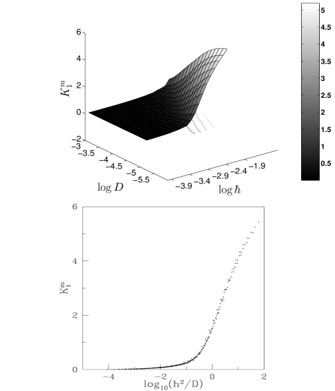
Figure 1: Top: Maximal Kullback-Liebler distance $K_{1}^{m}$ as a function of $\hbar$ and $D$, for the Quantum Cat Map. Note that small values reflect strong similarity between classical and quantum evolutions. Bottom: Same data plotted in terms of a composite parameter reflecting scaling behavior.

We illustrate the technique by considering a simple but extensively studied system, the noisy quantum Cat Map Josh ; koslovsky ; pb . The classical limit displays extreme (uniformly hyperbolic) chaos, and as such the system should be a member of a distinct universality class. The uniform hyperbolicity also precludes any dependence on initial conditions. The dynamics derive from the kicked oscillator Hamiltonian ford

$$H=p^{2}/2\mu+\epsilon q^{2}/2\sum_{s=-\infty}^{\infty}\delta(s-t/T).$$ (5)

restricted to the torus $0\leq q<a$, $0\leq p<b$, with the parameter constraints $Tb/\mu a=1$ and $-\epsilon Ta/b=1$. The chaos here results not from the non-linearity of the Hamiltonian but from the choice of (re-injected) boundary conditions. As such, the general equation Eq. (1) does not apply. However, the first quantum correction to the classical propagator for this system (for the the Fourier-transformed distribution) is of order $\hbar k$ for the Fourier mode $k$ Josh . The quantum-classical distance for this system then behaves as $\hbar\chi$, implying that fn2 $\zeta=\hbar^{2}\chi^{2}=\hbar^{2}\Lambda D^{-1}$. The top panel of Fig. 1 shows $K^{m}_{1}$ as a function of $\hbar,D$. It is clear the distance behaves as expected. For example, as $\hbar$ is increased, larger $D$ values are needed for the quantum and classical distributions to coincide. The lower panel shows the same data, plotted as a function of the single composite variable $\zeta=\hbar^{2}/D$. The reduction of the surface in the upper panel to a single function of $\zeta$ demonstrates the scaling relationship between $\hbar,D$. The accuracy of this scaling is reflected in the lack of any discernible spread around the curve. Remarkably, the scaling extends over many orders of magnitude in both parameters $\hbar,D$ and a considerable range in $K^{m}_{1}$.

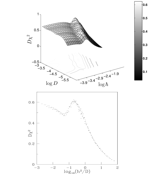
Figure 2: Top: This measure reflects the generation of fine-scale structure in the dynamics with larger values corresponding to classical dynamics. Bottom: Same data plotted in terms of a composite parameter. Note the same scaling as in Fig 1 and the coincidence of the transition region.

The functional dependence of $K^{m}_{1}$ on $\zeta$ shows a number of distinctive features. (i) $K^{m}_{1}$ is monotonic in $\zeta$, although as we argue below, there is no general reason to expect this. (ii) The quantum-classical distance is nonlinear in $\zeta$, with $K^{m}_{1}(\zeta)$ initially growing slowly as a function of $\zeta$, followed by a rapid transition at $\ln(\zeta)\approx 0$ or $\zeta\approx 1$. This boundary is consistent with previous results koslovsky ; pb ; ap . (iii) The distance $K_{1}$ is bounded due to the noise, and we see the expected saturation for higher values of $\zeta$. (iv) There appear to be distinct regimes corresponding to small (for $\zeta<1$) and large (for $\zeta>1$) quantum-classical distance. This last behavior is arguably generic as, in chaotic systems, a classical distribution develops fine-scaled structure very quickly ($\chi^{2}$ grows rapidly), increasing its entropy production rate as well as its sensitivity to external noise. For this class of systems, in the first regime ($\zeta<1$), a quantum distribution initially remains close to the classical and will also increase its entropy production rate, and consequently the rate at which it becomes a mixed state. Hence any quantum effects that develop will be suppressed by the noise and the quantum-classical distance will remain small for all times. In this regime, the environment minimizes the quantum-classical difference. In the second regime (for $\zeta>1$), the quantum distribution does not initially follow the classical distribution to finer scales, and does not become sensitive to noise. It thus remains far from classical even as the noise alters the classical system. Here, the environment exaggerates the differences between quantum and classical probability dynamics. As such, $\zeta\approx 1$ may be viewed as a ‘quantum-classical boundary’, with qualitatively different behavior on either side of it.

The general arguments above imply that similar scaling should be visible in all appropriately constructed measures of the quantum-classical distance. In Fig. 2 we show results for an alternate measure $D\chi^{2}$, which is related to the spreading of structure to finer scales. Unlike $K^{m}_{1}$ which compares classical and quantum evolution, this second measure is strictly quantum mechanical. The supremum value in time of $D\chi^{2}$ ($\equiv D\chi^{2}_{m}$) is considered with varying $\hbar,D$ and for the same time-scales as before (classically, we would get a constant physicaD ). Again, the precision and range of the scaling is remarkable. The qualitative conclusions are exactly the same as for $K^{1}_{m}(\zeta)$, with a similar rapid transition between large and small values of $D\chi^{2}_{m}$, happening again at $\zeta\approx 1$. That is, for small $\zeta$, the distribution is very sensitive to noise, changing rapidly as a function of $\zeta$ to low sensitivity. However, this curve has a distinctive dip near $\zeta\approx 1$, such that the peak is at finite $\zeta$. This has been seen previously 97_1 , and can be understood by the fact that for near-classical quantum dynamics, the quantum follows the classical distribution but carries interference fringes on top of the classical structure. As such, the quantum distribution can be more sensitive to noise than the classical counterpart. In particular, as above, $\rho_{W}\approx\rho_{c}+a\hbar\chi\rho$ where $a$ is some constant. Similarly, the quantum and classical $\chi^{2}$ are related as $\chi_{q}^{2}\approx\chi_{c}^{2}+a\hbar\chi^{3}$ so that to zeroth order $\chi_{q0}^{2}=\chi_{c}^{2}$, where the subscript on $\chi_{q}$ indicates the order. To first order, we substitute the zeroth order expression for $\chi^{3}$ to get $\chi_{q1}^{2}\approx\chi_{c}^{2}+a\hbar\chi_{c}^{3}$. Iterating this procedure, to second order we will get terms like fn3 $\chi_{q2}^{2}\approx\chi_{c}^{2}+a\hbar\chi_{c}^{3}(1+a\hbar\chi_{c})^{\frac{3}{2}}$. For small $a\hbar$ this becomes

$$\chi_{q}^{2} \approx \chi_{c}^{2}(1+a\;\hbar\chi_{c}+\frac{3}{2}a^{2}\;\hbar^{2}\chi_{c}^{2}+\frac{3}{8}a^{3}\;\hbar^{3}\chi_{c}^{3}+\ldots)$$ (6)

$$\approx \chi_{c}^{2}(1+a^{\prime}\;\zeta^{\frac{1}{2}}+b\;\zeta+c\;\zeta^{\frac{3}{2}}+\ldots)$$

where the constants $a^{\prime},b,c$ absorb all other constants and we have substituted $\hbar^{2}\chi^{2}=\zeta$. The initial effect of quantum dynamics is to reduce the value of $\chi^{2}$ and hence $a^{\prime}$ (and consequently $c$) must be negative valued constants, while $b$ is positive. For appropriate values of $a^{\prime},b,c$, Eq. (6) can indeed account for the shape of the curve seen in Fig. (2). Therefore, all measures of quantum-classical distance need not depend monotonically on the system parameters. However, the particular dependence shown is almost definitely not generic since it depends on the relevant constants being of the appropriate ratios.

These results provide definitive evidence of parameter scaling in QCT for chaotic systems, which may be used to clearly identify different regimes of quantum-classical correspondence. As such, these are the first steps towards identifying and using composite parameters in studying universal behavior in the quantum-classical transition for small $\zeta$ (the near-classical regime). The smoothness and breadth of the scaling results shown are likely to be a feature of the uniform hyperbolicity of systems like the Cat Map. Understanding how this is altered by less extreme dynamics is clearly the next step, both in terms of constructing $\zeta$ and well as exploring the dependences of computed measures on $\zeta$. In particular, a preliminary assessment of entirely different measures applied to the quantum Duffing problem indicates that similar scaling may exist there as well.

Acknowledgement - A.K.P. acknowledges with pleasure useful comments from Doron Cohen and Ivan Deutsch. The work of B.S. was supported by the National Science Foundation grant #0099431 and a grant from the City University of New York PSC-CUNY Research Award Program.

References

- (1) W. H. Zurek and J. P. Paz, Phys. Rev. Lett. 72, 2508 (1994); Physica 83 D, 300 (1995).
- (2) A. K. Pattanayak and P. Brumer, Phys. Rev. Lett. 79, 4131 (1997).
- (3) E. Ott, T.M. Antonsen and J.D. Hanson, Phys. Rev. Lett. 53, 2187 (1984).
- (4) D. Cohen, Phys. Rev. Abf 44, 2292 (1991).
- (5) A. R. Kolovsky, Phys. Rev. Lett. 76, 340 (1996).
- (6) A.K. Pattanayak, Phys. Rev. Lett. 83, 4526 (1999).
- (7) T. Bhattacharya, S. Habib, and K. Jacobs, Phys. Rev. Lett. 85, 4852 (2000).
- (8) S. Habib, K. Jacobs, H. Mabuchi, R. Ryne, K. Shizume, and B. Sundaram, Phys. Rev. Lett. 88, 040402 (2002).
- (9) A dependence of the QCT on implies such a scaling dependence exists in the parameter as well, for arbitrary . We may choose one coefficient (e.g., setting ) to determine the other two coefficients.
- (10) C. Beck and F. Schlögl, Thermodynamics of chaotic systems, (Cambridge University Press, N.Y., 1993).
- (11) A.K. Pattanayak, Physica D 148, 1 (2001).
- (12) Yuan Gu, Phys.Lett.A 149, 95 (1990); A. K. Pattanayak and P. Brumer, Phys. Rev. E56, 5174 (1997).
- (13) J. Wilkie, Ph.D. Dissertation (unpublished), University of Toronto, 1994.
- (14) J.Ford, G.Mantica and G.H.Ristow, Physica D 50, 493 (1991).
- (15) We set , and choose as discussed in fn1 above. Our figure has a logarithmic scale for , whence this choice affects only the aspect ratio of the figure.
- (16) In general, the expansion for around in terms of includes terms in arising from the higher-order terms in the relationship between and . For the argument that the relationship between and is nonlinear in , these may be neglected since they only add to the nonlinearity.