Abstract

We discuss an experiment conducted by Nesvizhevsky et al. As it is the first experiment claimed to have observed gravitational quantum states, it is imperative to investigate all alternative explanations of the result. In a student project course in applied quantum mechanics, we consider the possibility of quantummechanical effects arising from the geometry of the experimental setup, due to the ”cavity” formed. We try to reproduce the experimental result using geometrical arguments only. Due to the influence of several unknown parameters our result is still inconclusive.

1 Introduction

A wellknown property of quantum mechanics is the quantisation of the energy levels of a particle trapped in a potential well. For instance, the electromagnetic and the strong nuclear force create different kinds of potential wells and are responsible for many observed phenomena in nature, such as the structure of atoms and nuclei. This suggests that a splitting of the energy levels should also be observed for particles in the Earth’s gravitational field. But, since the gravitational field is much weaker, the effect should be subtle and hard to detect.

In a letter to Nature [Nev02], Nesvizhevsky et al. claim to have observed such quantum effects of gravity acting on ultracold neutrons (UCNs). They conducted an experiment in which the UCNs were allowed to flow through a cavity with a reflecting surface below and an absorber above. By measuring the number of neutrons exiting the experimental setup, they claim to have observed discrete energy levels. However, in their argument they seemingly disregard the modification due to the absorber, stating that it is “sufficiently perfect”. Further they argue that the discretisation is related to the sudden increase of neutrons coming through at distinct widths between the reflecting surface and absorber. However, since the UCNs are restricted by both the reflecting surface and the absorber, also the geometrical effects should be considered. The results might even be explained by geometrical arguments only.

The aim with this report is to show that by only using geometrical arguments, the effects observed by the scientist at Grenoble can be explained.

2 Background

Here we give a brief review of the experiment reported in [Nev02]. A similar experiment was first suggested by V.I. Luschikov and A.I. Frank in 1978 [Fra78]. We also discuss inconsistencies of their theoretical analysis and their results, giving us some ideas of how to approach an alternative explanation.

2.1 The experiment

The experiment was performed with UCNs flowing between a reflecting surface below, and an absorber above. The absorber and the “mirror” create a slit through which the neutrons pass, eventually reaching a detector at the other end of the experimental setup (Fig. 1). UCNs are essential to the experiment since they offer many advantages. For instance, they have an energy of about $10^{-7}\ \mathrm{eV}$, corresponding to a wavelength of $\sim$500 Å or a velocity of $\sim$10 m/s, allowing them to undergo total reflection at all angles against a number of materials. The low energy also allows for high resolution, and since neutrons have a lifetime of the order of 900 s, it is possible to store them for periods of 100 s or more. This makes UCNs available and suitable for research and experiments in fundamental physics. The leading research on UCNs is conducted at LANSCE, the Los Alamos Neutron Science Center, and at ILL, the Laue Langevin Institute, the latter holds the current “worldrecord” density of 41 UCNs/cm³.

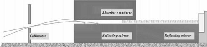
Figure 1: A schematic layout of the experiment [Nev00]. A horisontal beam of neutrons is collimated and enters the gap between the absorber and the mirror. Neutrons of certain energies eventually reach the detector on the right, while others are absorbed.

Nesvizhevsky et al. argue that when the neutrons are trapped in a potential formed by the mirror (an impenetrable ”floor”) and the Earth’s gravity there will be a discrete set of possible energy levels (Fig. 2). The four lowest energy eigenvalues are $E_{1}=1.41\ \mathrm{peV}$, $E_{2}=2.46\ \mathrm{peV}$, $E_{3}=3.32\ \mathrm{peV}$ and $E_{4}=4.08\ \mathrm{peV}$. For a theoretical treatment of this potential, see [Flu99].

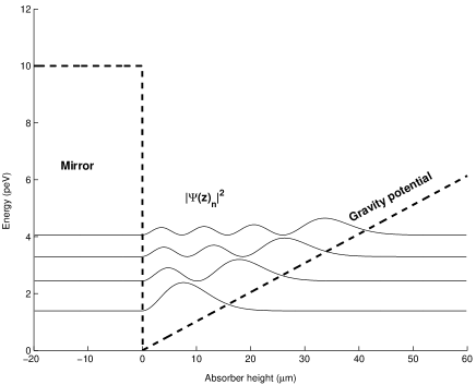
Figure 2: The energy versus the absorber height, with the four lowest energy eigenvalues indicated. The probability functions are plotted schematically. Our calculated eigenvalues are in accordance with the theoretical values in [Nev02].

The lowest eigenvalue $E_{1}$ corresponds to a classical height, $E_{1}=mgz$, of about 15 $\mu$m. This leads the group to predict that when the slitopening is less than this height no neutron transmission will occur. They argue that if the quantummechanical wavefunction has a spatial extension larger than the opening, it will not fit, and the neutrons have no chance of reaching the detector. In the experiment the group observed a stepwise increase in the number of detected neutrons as they increased the slit height. In particular they observed, as predicted, that when the slitopening was less than 15 $\mu$m no neutrons reached the detector, but that there occurred a sudden increase after 15 $\mu$m and another at about 20 $\mu$m. Their results are shown in Fig. 3.

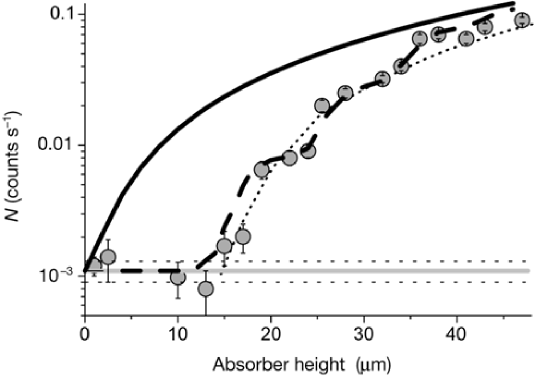
Figure 3: Neutron count versus the absorber height in the experiment of [Nev02]. The dots with error bars show the experimental data. The solid line is the expectation from a ”classical” analysis, while the dotted curve corresponds to a quantummechanical treatment with only the first state taken into account. For the dashed curve several states and level populations are considered.

The curves are from the theoretical analysis. The solid line is the fully classical treatment, where the neutron throughput does not have a lower threshold and is described by

$$N_{Classical}(z)\sim z^{1.5},$$ (1)

where $z$ is the absorber height. Thus the neutron count increases as $z^{1.5}$, since as the height is increased a larger spread of velocities of the neutrons is allowed. The dotted line is, according to [Nev02], the neutron count when only the lowest eigenstate is considered. This is merely a translation of the classical curve with the lowest threshold taken into account,

$$N_{\psi_{1}}\sim(z-z_{0})^{1.5},$$ (2)

where $z_{0}$ is the absorber height at which the slit becomes transparent to neutrons. This assumes that the neutrons behave ”classically” once allowed to penetrate the gap. The dashed line is the curve when level populations of all four lowest states were considered.

2.2 Reasons for further investigations

A first thing to point out is that, the energy eigenvalues have never been measured, i.e., all these results are entirely theoretical. So, the only data available to us are the neutron counts, $N$, at the detector as a function of the absorber height $z$.

The potential used in the analysis is $V(z)=mgz$, which is the classical gravitational potential of the Earth.

The absorber is thought to be perfect, removing the wavefunctions (i.e., the neutrons) completely when they extend into it. From a classical point of view, neutrons with different energies bounce off the mirror. The different energies will result in different heights. This is the classical explanation to why the higher states are missing. If one then looks at the true quantummechanical picture, the neutrons are now described by standing waves in the gravitational potential, and there are no ”bouncing” particles. Now the absorber must also be described by a potential and the classical argument will not be sufficient. The absorber could hence give a geometrical explanation for the quantum states.

The experimental statistics for larger slit widths is insufficient [Nev02], so we need consider, say, the two first steps, making the task of an alternative explanation a bit simpler.

3 Alternative explanations

In the first two subsections we try to recreate the energy eigenvalues obtained for a particle in the Earth’s gravitational field using only geometrical arguments. However, a more careful study of [Nev02], as well as contact with the experimental group, makes us believe that no energy eigenvalues have actually been measured. Instead of recreating the energy eigenvalues we tried to explain the jumps in the number of detected neutrons. This is presented in subsection 3.3.

3.1 Particle in a box

We start with a potential consisting of two infinite walls, this should be a fairly good approximation. The reflecting surface, the mirror, can be seen as an infinite wall but the absorber needs more consideration.

The problem is easy to solve analytically [Flu99] [Gas96], and the energies are given by

$$E_{n}=\frac{\hbar^{2}\pi^{2}n^{2}}{2ma^{2}},$$ (3)

where $a$ is the box width. Thus, the first energy eigenvalue of a neutron trapped in a box with infinite walls and a width of 15 $\mu$m is $E_{1}=0.9\ \mathrm{peV}$. The first energy eigenvalue of a neutron in the Earth’s gravitational field, $E_{1grav}=1.41\ \mathrm{peV}$ [Nev02], is in the same range. Therefore the assumption that we could approximate the experimental setup with a infinite well is not quite correct, but it gives us a hint that it might be possible to find a potential that could reproduce all the energy eigenvalues of a neutron in a ”gravitational field” with only geometrical arguments. In the next section we try to modify the infinite well with, a better approximation of the absorber.

3.2 Energy eigenvalues

The best results are obtained by using a so-called Wood-Saxon potential, to approximate the absorber. However, the only way to get the gravity potential results was to allow the Wood-Saxon potential to be very close to the gravity potential itself. This of course, was not the result we were hoping for. Consequently we were forced to extend our discussion further. As mentioned before we received more information about the experiment and therefore instead of reproducing the energy eigenvalues, we only needed to obtain the correct neutron counts and this will be described in the next section.

3.3 Neutron counts

In order to reproduce the count rate we had to consider the length (10 cm) of the experimental setup. We further assumed that a neutron traversing the experimental setup is absorbed as

$$N(x,z)=N_{max}(z)e^{-k(z)x},$$ (4)

where $N_{max}(z)$ is the neutron density at the entrance $x=0$, $x$ is the distance along the mirror, and $k(z)$ is an absorber parameter related to how much the neutron wavefunction is inside the absorber. The crucial condition that must be satisfied is of course, that when the distance $z$ is less than 15 $\mu$m no neutrons should be able to reach the detector, i.e., $N(x,z)$ must be close to zero.

In a distance of $\Delta x$, an amount of $1-A(z,\Delta x)$ neutrons will be absorbed, yielding

$$N(x_{2},z)=(1-A(z,\Delta x))N(x_{1},z).$$ (5)

Hence we get

$$A(z,\Delta x)=1-e^{-k(z)\Delta x},$$ (6)

where $A(z,\Delta x)$ is the area of the probability functions inside the absorber. The function $k(z)$ can be obtained from the experimental data with the help of Equation (4), giving

$$k(z)=-\frac{1}{L}\ln\left[\frac{N_{out}(x,z)}{N_{max}(z)}\right],$$ (7)

where $L$ is the length of the cavity. If we consider only the lowest state $\psi_{1}(z)$, we must recreate $N_{out}(z,x)$ as the dotted curve in Fig. 3. See Appendix A for a simulation considering only the first state. On the other hand, when using the four lowest states, the outcome must be the dashed line in Fig. 3. This case yields the probability function

$$|\psi|^{2}=C_{1}|\psi_{1}|^{2}+C_{2}|\psi_{2}|^{2}+C_{3}|\psi_{3}|^{2}+C_{4}|\psi_{4}|^{4},$$ (8)

with the normalisation condition

$$C_{1}+C_{2}+C_{3}+C_{4}=1.$$ (9)

Since we do not know the level population parameters $C_{i}$, we have the freedom to choose them to make our model agree with the experimental data.

3.4 Combination

There is also the possibility that the gravity potential indeed effects the quantum states of the neutrons in this experiment. However we would like to, unlike the group conducting the experiment, consider the effects from the absorber as well. This only changes the appearance of the potential in Fig. 2, but not our principle model.

4 Conclusions and further investigations

The main problem in our attempts to explain the results with a geometrical model is that $N_{max}(z)$ is unknown, depending on the spread of energies in the neutron beam. Other difficulties are finding realistic potentials describing the absorber and that, due to a lack of data, our treatment is static. The time independence will exclude important phenomena such as tunnelling effects.

Hence our results are inconclusive. We have not yet determined a potential satisfying our requirements and we await the next report from the experimental group, hoping it will contain the information we need.

We propose the following improvements of the experiment:

• Rotating the experimental setup by $90^{\circ}$ keeping everything else, especially the transverse neutron energies, constant. If the same result occurs it would indicate that the result is due only to the geometry of the experimental setup as no gravitational quantum states can form in this case.

• Increasing the length of the cavity. If the output would decrease it might confirm our theory of an absorption per unit length.

• A measurement of where the neutrons strike the detector. The probability distribution should reflect $|\psi|^{2}$ (since there is a standing neutron wave, the neutron is not falling in a classical sense).

Appendix A Simulation of a potential

We start by simulating a potential describing the absorber, considering only the lowest state. With our algorithm we obtain the first eigenfunction (Fig. 4) for $z=15\ \mu$m.

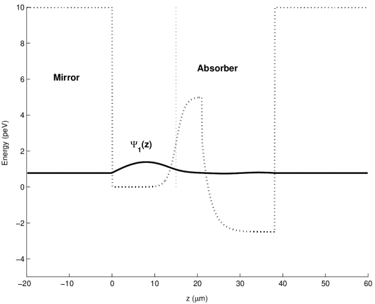
Figure 4: A simulation of a potential describing the absorber with the output of the first eigenfunction.

Then we calculate the normalised probability function and its area inside the absorber,

$$A(15\ \mu\textrm{m},\Delta x)\simeq 0.0173\ \textit{{area units}}.$$

By assuming $L=10$ cm and $N_{max}(z)=0.3$ the function $k(15\ \mu\textrm{m})$ can be determined as

$$k(15\ \mu\textrm{m})\simeq 0.54991,$$

where we have obtained $N_{out}(10\ \textrm{cm},15\ \mu\textrm{m})$ from the experimental data. Finally we can determine $\Delta x$ as

$$\Delta x\simeq 0.0320259\ \textrm{cm}.$$

Now we compare the theoretical $A(z,\Delta x)$, obtained from the experimental data, with the simulated areas which we get with our algorithm, see Table 1.

Slit width ($\mu\textrm{m}$)	Simulated area (a.u.)	Theoretical area (a.u.)
$20$	$0.0252$	$0.01245$
$30$	$0.0031$	$0.08333$

Table 1: A comparison of the areas obtained from the theory versus the simulated ones.

The simulation and comparison of the areas show the difficulties we had with our model. With the assumption that $N_{max}(z)=0.3$, our area inside the absorber decreases faster than the theoretical one when $z$ is increased. We must find a suitable potential describing the absorber so that the two areas are the same for all $z$. Also, the cutoff below $z=15\ \mathtt{\mu}$m must be satisfied.

References

- [Nev00] V. Nesvizhevsky et al., Search for quantum states of the neutron in a gravitational field : gravitational levels, Nucl. Instrum. Methods Phys. Res. 440 (2000) 754.
- [Nev02] V. Nesvizhevsky et al., Quantum states of neutrons in the Earth’s gravitational field, Nature 415 (2002) 297.
- [Flu99] S. Flügge, Practical Quantum Mechanics, Springer-Verlag, 1999.
- [Fra78] V. I. Luschikov & A. I. Frank, Quantum effects occurring when ultracold neutrons are stored on a plane, JETP Letter 28 (1978) 559.
- [Gas96] S. Gasiorowicz, Quantum Physics, John Wiley & Sons Inc., 1996.
- [Sch02] B. Schwarzschild, Ultracold Neutrons Exhibit Quantum States in the Earth’s Gravitational Field, Physics Today 55 (2002) 20.