Manipulating the shape of electronic non-dispersive wave-packets in the hydrogen atom: numerical tests in realistic experimental conditions

Abstract

We show that combination of a linearly polarized resonant microwave field and a parallel static electric field may be used to create a non-dispersive electronic wavepacket in Rydberg atoms. The static electric field allows for manipulation of the shape of the elliptical trajectory the wavepacket is propagating on. Exact quantum numerical calculations for realistic experimental parameters show that the wavepacket evolving on a linear orbit can be very easily prepared in a laboratory either by a direct optical excitation or by preparing an atom in an extremal Stark state and then slowly switching on the microwave field. The latter scheme seems to be very resistant to experimental imperfections. Once the wavepacket on the linear orbit is excited, the static field may be used to manipulate the shape of the orbit.

PACS: 05.45.+b, 32.80.Rm, 42.50.Hz

1 Introduction

Atomic wavepackets form a bridge which allows to understand the mutual relations between the classical and the quantum world [1, 2, 3]. Typically (i.e. with the notable exception of the harmonic oscillator) any initially localized wavepacket (which mimics a classical particle) will have its center of mass follow a classical trajectory at short time, but will progressively spread in time. Recent years have brought several attempts to overcome the spreading.

The wavepacket spreading is classical in character and is due to the nonlinearity of the Hamiltonian, or saying it differently, the fact that trajectories with different energies evolve with different frequencies [3]. To overcome the classical spreading of a bunch of particles, the phenomenon of nonlinear resonance can be used (e.g while guiding particles in accelerators). The idea is very simple: a classical nonlinear system periodically driven by an external perturbation displays resonances when the period of the external driving matches the period of the unperturbed motion. In a region of phase space called nonlinear resonance island, the internal motion of the system becomes locked on the external drive. This motion in the resonance island is similar to pendulum oscillations. The corresponding quantum description was first given by Berman and Zaslavsky [4] and later readressed by Henkel and Holthaus [5, 6], who also gave the semiclassical interpretation. For realistic systems, first studies involved the hydrogen atom driven by either a linearly [7, 8] or circularly [9, 10, 11] polarized microwave field. In the latter situation, a particularly simple picture may be obtained since, in the frame rotating with the microwave electric field, the Hamiltonian becomes time independent and the center of the pendulum island becomes a fixed point of the dynamics. This allows for an approximate description of the states localized near the stable fixed point using Gaussian wavepackets, termed then Trojan states [9].

Several properties of nondispersive wavepackets have been analysed recently. The mixed semiclassical/quantum description is particularly convenient. Because of the time periodicity of the driving, the Floquet theorem [12] can be used: it ensures the existence of a basis of states (the eigenstates of the Floquet Hamiltonian) which evolve periodically in time, and that any solution of the time-dependent Schrödinger equation can be expanded in a simple linear combination of these quasienergy eigenstates. If a single quasienergy eigenstate is initially localized, it will preserve this localization during the temporal evolution or, more precisely, recover it every period of the drive [10], and thus overcome the long-time spreading. From semiclassics, such states can be constructed as localized inside the nonlinear island and thus constitute nondispersive wavepackets locked on the external driving. Because they are built from two robust structures (the classical resonance island and the basis given by the Floquet theorem), the nondispersive wavepackets are robust versus any small perturbation not taken into account in the preceding approach. For example, for microwave driven atoms, the nondispersive wavepacket states are resistant to any geometrical imperfection in the field direction, amplitude or polarization, and protected from direct fast ionization by the resonance island (they can however ionize after tunneling outside the island and their lifetimes exhibit interesting fluctuations [11, 13]). Their decay due to spontaneous emission of photons has also been analysed [14, 15, 16].

These wavepacket states have most probably already been prepared in experiments studying the microwave induced ionization of hydrogen atom. Indeed, atoms were found to be relatively stable against ionization for microwave frequency close to Kepler frequency [17, 18, 19, 20]. However, those experiments were addressing different issues and, most probably, populated several Floquet states at once. For an unambiguous identification of nondispersive wavepackets, special preparation (as well as detection) schemes have to be envisioned. In fact, for wavepackets driven by a circularly polarized microwave field, such a scheme has been proposed quite early [10]. It requires the preparation of an atom in an initial Rydberg circular state, followed by a slow turn on of the circularly polarized microwave. This scheme has been simulated numerically for realistic parameters [21] but, up till now, no experimental test has been made.

It would be desirable to simplify the proposed scheme, especially to avoid the initial preparation of a circular state, which is possible but not trivial. By contrast, it is much simpler to excite a Rydberg state where the electron probability near the nucleus is important: a direct optical excitation from the ground state or a low excited state is simple and convenient. Moreover, because of the monochromatic character of the laser sources, it is rather simple to excite selectively the desired Rydberg state and not its neighbors. Thus, the simplest idea is to change the classical electron trajectory (on which the nondispersive wavepacket is built) to an elongated Kepler orbit hitting the nucleus. Such a nondispersive wavepacket can be easily achieved using a resonant microwave field linearly polarized along the degenerate Kepler orbit. There is however a undesirable side effect: the motion along the polarization axis is transversally unstable, that is any deviation from strict alignment of the electron along the microwave field will be exponentially amplified with time. This problem may be overcome by addition of a static electric field, parallel to the polarization axis as shown by us using a semiclassical approach [24]. The resulting situation is very attractive from the experimental point of view. In [24], we proposed two possible experimental schemes: either the direct optical excitation of the “linear” nondispersive wavepackets in the presence of both the linearly polarized microwave field and the stabilizing static field (scheme I) or the excitation of a convenient Stark state (in the presence of the static field only) followed by an adiabatic turn on of the microwave field (scheme II). Scheme I is simpler, but might be less convenient in a real experiment because it requires that the laser beam is sent inside the microwave cavity, which may be difficult. Scheme II requires some control on how the microwave field is turned on. Once the “linear” nondispersive wavepacket is excited by either of the two schemes, a subsequent decrease of the static field can lead to an “elliptical” nondispersive wavepacket, i.e. localized on an elliptical Kepler trajectory of arbitrary eccentricity and, in the limit of vanishing static field to a “circular” nondispersive wavepacket. The aim of this paper is to explore the feasibility of such schemes in a real experiment. We will use realistic parameters and the combination of a semiclassical approach (in order to get the orders of magnitudes and a physical picture of what is going on) and of full quantum numerical simulations (which provide accurate numbers). Such an analysis reveals also possible experimental difficulties overlooked in the semiclassical discussion.

A very similar experiment has been performed by Bromage and Stroud [22] who, starting from an extremal Stark state of the sodium atom, excited a wavepacket by applying a short electromagnetic half-cycle pulse which localized an electron on a highly eccentric orbit. After excitation, there was no mechanism to prevent the wavepacket from spreading. Nevertheless, the authors observed a few nice oscillations in the ionization signal reflecting the classical motion of the electron. Thus, it seems that only one step further is needed to obtain a nondispersive wavepacket in the laboratory. Namely the short pulse excitation should be replaced by a slow turn on of the microwave field whose presence afterwards assures the nonspreading character of the created wavepacket.

2 The quasi-energy spectrum at fixed static and microwave fields: confrontation of semiclassical and quantum results

We consider an hydrogen atom exposed to both a static electric field and a linearly polarized microwave field parallel to the static field. The Hamiltonian of the system reads (in atomic units, with the fields along the $z$ axis):

$$H=\frac{{\mathbf{p}}^{2}}{2}-\frac{1}{r}+Fz\cos(\omega t)+F_{s}z,$$ (1)

where $F$ and $\omega$ stand for the amplitude and frequency of the microwave field respectively, while $F_{s}$ is the amplitude of the static field. The system is invariant under rotation around the $z$ axis, and the angular momentum projection on this axis is consequently conserved. In the following, we will assume for simplicity $L_{z}=0.$ Similar conclusions can be reached for low values of $L_{z}.$

The Hamiltonian (1) is time-periodic; the Floquet theorem [12] implies that any solution of the Schrödinger equation can be written as a linear combination of the Floquet eigenstates. Those are time-periodic (with period $2\pi/\omega$) eigenfunctions $|\phi_{\alpha}(t)\rangle$ of the so-called Floquet Hamiltonian operator

$${\cal H}|\phi_{\alpha}(t)\rangle=\left(H-i\frac{\partial}{\partial t}\right)|\phi_{\alpha}(t)\rangle=\varepsilon_{\alpha}\ |\phi_{\alpha}(t)\rangle,$$ (2)

where $\varepsilon_{\alpha}$ are the quasienergies of the system. Thus the preparation of an atom in a single Floquet state ensures that the electronic density evolves periodically in time. However not every eigenstate $|\phi_{\alpha}(t)\rangle$ corresponds to a well localized electron propagating on a classical trajectory. To find which Floquet states are the nondispersive wavepackets, we need a semiclassical approach. In order to study the classical dynamics of such a time-dependent system, we need to define the extended phase space [23] where one deals with the additional momentum $P_{t}$ conjugate to the $t$ (time) variable. The temporal evolution is described by the Hamiltonian function ${\cal H}=H+P_{t},$ which is the classical analog of the quantum Floquet operator defined in eq. (2).

Consider a hydrogen atom illuminated by a microwave field of frequency:

$$\omega=\frac{1}{n_{0}^{3}}.$$ (3)

$n_{0}$ is the effective principal quantum number which is resonant with the external driving, that is such that the unperturbed Kepler motion has the frequency $\omega_{K}=\omega$ (in the classical language) or such that the microwave perturbation is almost resonant with the transitions to the $n_{0}^{\prime}=n_{0}\pm 1$ neighboring states (in the quantum language).

At large microwave field, the classical phase space structure may be extremely complicated with interleaved regions of chaotic and regular motion. At relatively small microwave field – the situation we are interested in – the resonance between the driving frequency and the frequency of the unperturbed motion leads to a strong perturbation of the system and the creation of a stable island in phase space centered on a periodic orbit at exactly the frequency $\omega$. There, the effect of non resonant term (which are responsible for the onset of chaos at strong field) can be safely neglected. In this so-called secular approximation, it is assumed that the motion in the resonance island is much slower than the Kepler motion itself. The Hamiltonian can be rewritten in the unperturbed action-angle coordinates $(I,\theta,L,\psi)$ which describe the classical Kepler motion. The total action $I$ is the classical equivalent of the principal quantum number (so that the Hamiltonian of the unperturbed hydrogen atom is $-1/2I^{2}.)$ The conjugate angle $\theta$ describes the motion along the classical Kepler orbit (it evolves periodically at a constant angular velocity $\omega_{K}$). The other pair of action-angle coordinates $(L,\psi)$ describes the parameters of the classical Kepler ellipse, i.e. the total angular momentum $L$ related to the eccentricity by

$$e=\sqrt{1-\frac{L^{2}}{I^{2}}},$$ (4)

and the conjugate angle $\psi$ between the major axis of the classical Kepler ellipse and the field axis. A convenient approach is to switch to the rotating frame defined by:

$$\hat{\theta}=\theta-\omega t$$ (5)

$$\hat{P}_{t}=P_{t}+\omega I$$ (6)

because $\hat{\theta}$ appears as a slowly varying variable. The secular approximation is to neglect all terms in the Hamiltonian which oscillate at the microwave frequency or its harmonics. The effective Hamiltonian function describing the motion in the stable resonant island (for details see [3, 24, 25]) thus reads:

$${\cal H}_{\mathrm{sec}} = \hat{P}_{t}-\frac{1}{2I^{2}}-\omega I-\frac{3eF_{s}I^{2}}{2}\cos\psi$$ (7)

$$+ FI^{2}\left\{-J^{\prime}_{1}(e)\cos\psi\cos\hat{\theta}+\frac{\sqrt{1-e^{2}}J_{1}(e)}{e}\sin\psi\sin\hat{\theta}\right\}$$

where $J_{1}$ and $J^{\prime}_{1}$ denotes the Bessel function and its derivative, respectively.

Having the effective Hamiltonian, the last stage is to quantize the system. The radial motion, i.e. in the $(I,\hat{\theta})$ space, effectively decouples from the slow angular motion in the $(L,\psi)$ space. In effect, one can quantize the system in the spirit of the Born-Oppenheimer approximation, i.e. first quantize the radial motion keeping the secular motion frozen [27, 25], using the results to construct an effective potential for the motion in the $(L,\psi)$ space. In the limiting case when the motion in the $(I,\hat{\theta})$ space is harmonic such a procedure was followed in [24]. This is however not suitable for very low microwave fields. We give in the appendix the derivation and results in the general case. It should also be noted that, because the Coulomb potential is an homogeneous function (of degree $-1$) of the position while both the static and the microwave field interaction Hamiltonians are homogeneous functions of degree 1, there exist a classical scaling invariance law which allows to express the classical dynamics with the scaled quantities:

$$F_{0} = Fn_{0}^{4},$$ (8)

$$F_{s,0} = F_{s}n_{0}^{4},$$ (9)

$$L_{0} = \frac{L}{n_{0}}.$$ (10)

We have chosen to perform all numerical calculations (semiclassical and quantum) for $n_{0}=60.$ This value corresponds to the principal quantum number of Rydberg states prepared in a typical experiment. The corresponding resonant microwave frequency is $1/(60)^{3}$ in atomic units, i.e. 30.48 GHz. This is in the microwave regime where efficient high-quality sources are available. The electric field amplitude such that $F_{0}=0.01$ (a typical value to be used in an experiment, see below) is $0.01/(60)^{4}$ in atomic units, i.e. 4 V/cm. Producing a static or microwave field with such an amplitude is not a problem in a real experiment.

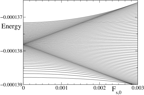
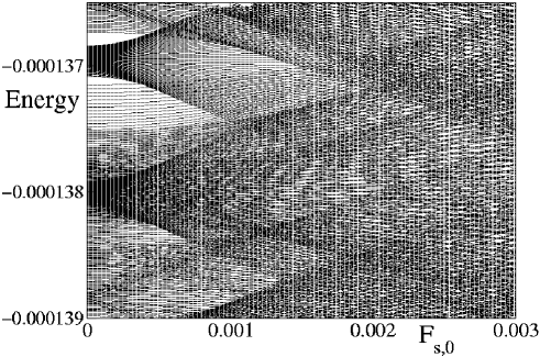
Figure 1: Quasienergy levels of the hydrogen atom exposed to parallel static and microwave fields as a function of the scaled static field $F_{s,0}$ for $n_{0}=60$ (microwave frequency 30.48 GHz) and fixed scaled microwave field amplitude $F_{0}=0.015$ (i.e. 6V/cm). The upper panel shows the levels of the $n=60$ manifold calculated using a semiclassical approach. The highest level of the manifold is the non-dispersive electronic wavepacket. For $F_{s,0}=0,$ it propagates along a circular trajectory. At increasing $F_{s,0},$ it smoothly turns into an elliptical non-dispersive wavepacket – that is a wavepacket propagating along an elliptical trajectory – and finally to a linear wavepacket propagating along the field axis. The lower panel shows the quasienergy levels obtained from an exact numerical diagonalization of the Floquet Hamiltonian. The levels belonging to the $n=60$ manifold almost coincide with the semiclassical prediction.

In Fig. 1, we show the quasienergy levels of the 60 states belonging to the resonant $n=60$ manifold as a function of the scaled static field $F_{s,0},$ for a fixed scaled microwave amplitude $F_{0}=0.015.$ For this calculation, we used the semiclassical approach described in the appendix. It is essentially identical to Fig. 2 of [24], for slightly different field values, but the general Mathieu quantization (described in the appendix) was used instead of the harmonic approximation used in [24]. The purely quantum quasienergy spectrum – obtained from numerical diagonalization of the Floquet Hamiltonian – is also shown in Fig. 1. It is remarkably similar to the semiclassical spectrum for the $n=60$ manifold. However, the total quantum spectrum is very congested, with plenty of other manifolds superimposed. These manifolds correspond to lower or higher principal quantum numbers shifted (in energy) by an integer multiple of the microwave frequency $\omega.$ It happens that, by chance, some of these manifolds overlap with the $n=60$ manifold. The most striking result is that these manifolds overlap but (almost) do not interact! Indeed, a careful inspection shows that there are no level crossings but rather very small avoided crossings (invisible at the scale of the figure). This is easily understood from the (semi)classical dynamics. Indeed, the nonlinear resonance island isolates the non-dispersive wavepackets from other states localized outside the island. In quantum mechanics, they are coupled only by tunneling, a typically very weak process responsible for the tiny avoided crossings.

The usefulness of the semiclassical approach must be emphasized. Without the guideline it provides, it would be impossible to recognize the $n=60$ manifold and identify the non-dispersive wavepackets in the mess of lower panel in Fig. 1. A further test of the accuracy of the semiclassical approximation is provided by a direct comparison of the numerical prediction for the quasienergy levels with the exact quantum levels. The difference is plotted in Fig. 2 for the upper state of the $n=60$ manifold, as a function of the scaled static field. The energy difference is plotted in units of the mean level spacing, which is here of the order of $2/n_{0}^{4}$ [10]. For all field values, it is smaller than 10% of the mean level spacing and it evolves essentially smoothly with the field. This implies that the semiclassical approximation catches most of the physics of the system. It also means that it can be used to easily find a state of interest among all energy levels obtained from a numerical diagonalization. More importantly, for $n_{0}=60,$ the energy difference between the semiclassical and quantum results is about $10^{-8}$ atomic units, corresponding to a frequency difference of 60 MHz. In a real experiment, the semiclassical prediction will thus gives a very useful indication for exciting the right spectral line.

Figure 2: Difference between the semiclassical prediction and quantum results for the energy of the non-dispersive wavepacket of the hydrogen atom in the presence of parallel microwave and static electric field, as a function of the scaled static field amplitude $F_{s,0}$. The parameters are those of figure 1, that is $n_{0}=60,F_{0}=0.015$. The energy difference $\Delta$ is plotted in units of the mean level spacing of the Floquet Hamiltonian, estimated to be equal to $2/n_{0}^{4}.$ $\Delta$ is much smaller than one, which proves the high-quality of the semiclassical approximation.

In zero static field (left of figure 1), one can see the manifold of states created in the presence of the microwave field only, with low-energy states associated with the weakest interaction with the microwave and consequently to the worst localization along the Kepler orbit (the latter being orbits mainly perpendicular to the field direction). In the middle of the manifold, one can see a local minimum spacing associated with the hyperbolic point at $(L=0,\psi=0)$, i.e. the degenerate linear Kepler orbit along the microwave field axis. As mentioned above, this motion is transversally unstable. The corresponding Floquet eigenstates are thus well localized longitudinally (they form nice wavepackets propagating back and forth) but poorly localized angularly. At the top of the manifold, there are states with maximum longitudinal localization and trajectories close to circular. Note, however, that these are $L_{z}=0$ states and that the circular trajectory is in the plane containing the quantization axis, so that the total wavefunction is localized on a sphere in the three-dimensional space, in sharp contrast with the so-called “circular” states (for pure hydrogen) which are localized on a circle perpendicular to the quantization axis or their combinations building Trojan-like [9, 10] wavepackets for circularly polarized microwave.

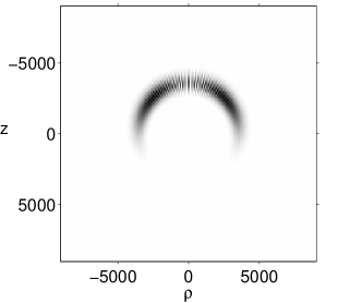
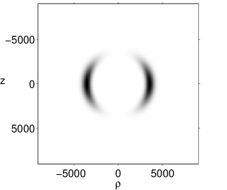
Figure 3: The wavepacket (the highest single Floquet state of the $n=60$ manifold in Fig. 1) obtained from diagonalization of the Floquet Hamiltonian for scaled microwave field amplitude $F_{0}=0.015$ and no static field $F_{s,0}=0.0$ and different phases of the microwave field (top-left $\varphi=0$, top-right $\varphi=\pi/4$, bottom-left $\varphi=\pi/2$ and bottom-right $\varphi=\pi$). The wavepacket is a torus pulsating on a sphere between the north and the south poles – the figure shows a cut along an arbitrary plane containing the $z$ axis multiplied by $\rho$ to simulate the density in cylindrical coordinates. The $\rho$ on the horizontal axis is either $x$ or $y$ or any other direction in the $xy$ plane. The scales are in atomic units.

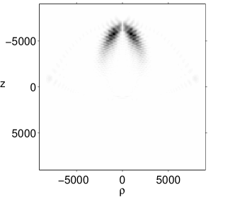
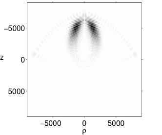
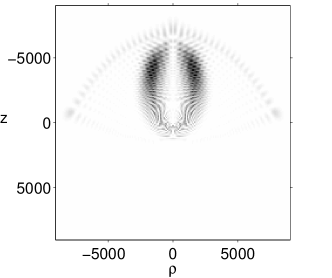
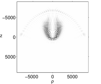
Figure 4: The wavepacket (the highest single Floquet state of the $n=60$ manifold in Fig. 1) obtained from diagonalization of the Floquet Hamiltonian for scaled microwave field amplitude $F_{0}=0.015$ and scaled static field $F_{s,0}=0.00255$ and different phases of the microwave field (top-left $\varphi=0$, top-right $\varphi=\pi/4$, middle-left $\varphi=\pi/2$, middle-right $\varphi=5\pi/8$ bottom-left $\varphi=3\pi/4$ and bottom-right $\varphi=\pi$). For this static field value, the nearby avoided crossing leads to a contamination of the wavepacket by another state. The wavepacket traces an elliptical trajectory. The scales are in atomic units.

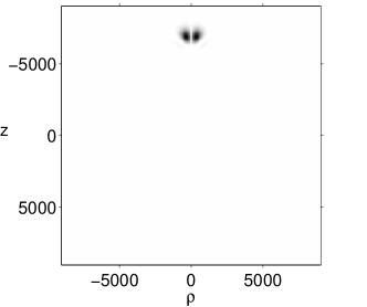
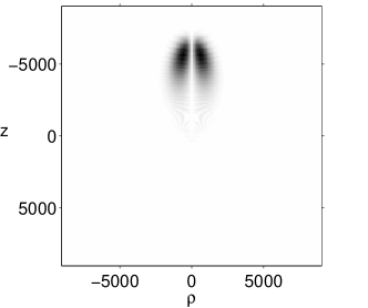
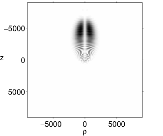
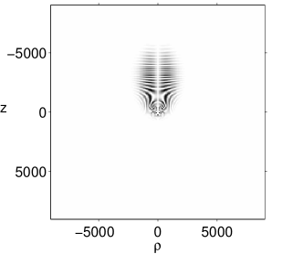
Figure 5: The wavepacket (the highest single Floquet state of the $n=60$ manifold in Fig. 1) obtained from diagonalization of the Floquet Hamiltonian for scaled microwave field amplitude $F_{0}=0.015$ and scaled static field $F_{s,0}=0.003$ and different phases of the microwave field (top-left $\varphi=0$, top-right $\varphi=\pi/4$, middle-left $\varphi=\pi/2$, middle-right $\varphi=5\pi/8$ bottom-left $\varphi=3\pi/4$ and bottom-right $\varphi=\pi$). The wavepacket follows a linear trajectory along the field axis. The scales are in atomic units.

Of special interest is the upper state of the manifold as it has maximum localization in the resonance island, but also maximum localization on the classical circular trajectory in the $(\rho,z)$ plane. Its temporal evolution over one period of the microwave field, is shown in Fig. 3. The plot is obtained from an exact numerical diagonalization of the Floquet Hamiltonian, following the techniques described in [26]. One clearly sees the nondispersive wavepacket character of this state, which is localized both in the $\rho$ and $z$ directions at all times, even extremely long (its evolution is periodic by construction). As expected, the wavepacket propagates along the circular trajectory with radius given by the Bohr orbit for $n_{0}=60$, that is roughly 3600 atomic units. In the plot, the wavepacket appears with two components symmetric with respect to the $z$ axis. Actually, the figure is a cut of the three-dimensional electronic density by a plane containing the field axis (multiplied by $\rho$ to simulate the probability density in cylindrical coordinates) and – due to the azimuthal symmetry – must appear symmetric. In the three-dimensional world, the wavepacket rather appears as a ring propagating back and forth between the north and south poles of a sphere. The fringes visible at $t=0$ and $t=\pi/\omega$ are due to interferences between ingoing and outgoing parts of the wavepacket.

When the static field is turned on, the manifold expands. One clearly sees inside the manifold the local shrinking of the mean level spacing corresponding to the hyperbolic fixed points of the transverse dynamics in the $(L,\psi)$ plane. The upper state of the manifold is associated with the elliptic (stable) fixed point with maximum effective energy in the $(L,\psi)$ plane, which is located at $\psi=\pi$ (major axis of the Kepler orbit along the field) with total angular momentum $L$ decreasing with increasing static field. Hence, this state is predicted to be a nondispersive wavepacket with optimum longitudinal localization; it evolves from a “circular” wavepacket at $F_{s}=0$ to a “linear” wavepacket above $F_{s}\simeq 0.2F$ passing through intermediate “elliptical wavepacket”. This is fully confirmed by the exact numerical diagonalization of the Floquet Hamiltonian at various static field strengths. We show in figures  4 and  5 snapshots of the electronic densities, which clearly show the evolution on the classical trajectory as well as the excellent longitudinal localization of the non-dispersive wavepackets. Note, however, at $F_{s,0}=0.00255,$ a small contamination of the wavepacket by a neighboring state (the field value is intentionally chosen in the vicinity of a very small avoided crossing) visible by a small ring of electronic density at 8000 Bohr radii.

Around $F_{s,0}=0.0028,$ the wavepacket turns into the “linear” wavepacket. This transition (actually an inverse pitchfork bifurcation where the linear trajectory turns from unstable to stable while the elliptical trajectory coalesces with the linear one and disappears) is visible in both the semiclassical and the quantum energy spectra as a local minimum in the energy level spacing. Above this bifurcation, the microwave field appears essentially as a perturbation of the static field, and the whole manifold is approximately composed of equally spaced levels, like a usual Stark manifold of the hydrogen atom.

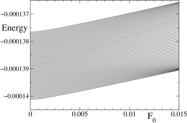
Figure 6: Quasienergy levels of the hydrogen atom exposed to parallel static and microwave fields. They are here plotted for $n_{0}=60$ – i.e. microwave frequency 30.48 GHz – static field strength $F_{s,0}=Fn_{0}^{4}=0.003$ (i.e. 1.2V/cm), as a function of the scaled microwave field amplitude $F_{0}.$ The levels of the $n=60$ manifold are calculated using the semiclassical approximation described in the appendix. The highest level of the manifold is the non-dispersive electronic wavepacket. For $F_{0}=0,$ it is the extreme blue shifted Stark state localized along the field axis. As the microwave field is increased, the electronic density progressively concentrates and builds a non-dispersive wavepacket evolving periodically along a linear Kepler trajectory.

In Fig. 6, we show another level dynamics, now at fixed scaled static field $F_{s,0}=0.003$ and increasing scaled microwave field. For clarity, only the semiclassical spectrum is shown, the exact quantum result being almost indistinguishable. At zero microwave field strength, we have a pure Stark manifold; at increasing microwave field, one first sees a quadratic (in $F_{0}$) increase of the quasienergies, in accordance with the weak-field limit discussed in the appendix followed by a linear regime (the strong-field regime discussed in the appendix). The most important information is that all levels are practically parallel in the full range, meaning that one passes very smoothly from a stationary state (at $F_{0}=0$) to a well localized non-dispersive wavepacket at $F_{0}=0.015.$ This smoothness is another illustration of the robustness of the non-dispersive wavepackets. Note that, for the highest state of the manifold, there is no angular evolution of the electronic density when the microwave field is turned on. Already at $F_{0}=0$ the extreme blue shifted Stark state is well localized along the field axis. By increasing the microwave field, one gains progressive longitudinal localization along the orbit as the resonance island in the $(I,\theta)$ plane grows.

3 Quantum dynamics with slowly changing amplitudes of static and microwave fields

From the preceding section, it is clear that the exact quantum level dynamics is extremely close to the semiclassical prediction as well as being very smooth with tiny avoided crossings only. This implies that the idea of manipulating the non-dispersive wavepackets by slowly changing the microwave or static field amplitudes is a realistic one.

Let us consider the scheme II introduced above. The first step is the direct optical excitation of a extreme blue shifted Stark state in the absence of microwave field. In the plot of Fig. 6, this is the highest state of the manifold. As its wavefunction is elongated along the field axis and has a significant value close to the nucleus, optical excitation from a low lying state is possible with high efficiency. Increasing the microwave field value is tantamount to adiabatically following the highest state of the manifold from the left to the right of Fig. 6. As the level dynamics is extremely smooth, a very efficient adiabatic transfer is likely to be possible. In order to test this hypothesis, we performed a numerical resolution of the time-dependent Schrödinger equation in the presence of a static time-independent field ($F_{0,s}=0.003$) and a microwave field with slowly increasing amplitude. We chose the following shape for the microwave field turn-on:

$$F_{0}(t)=F_{0}^{\mathrm{max}}\sin^{2}\frac{\pi t}{2T_{1}}$$ (11)

with $F_{0}^{\mathrm{max}}=0.015$ and $T_{1}=600$ microwave periods. The choice of the precise value of the switching time $T_{1}$ is by no means critical.

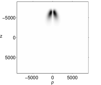
Figure 7: Preparation of a non-dispersive wavepacket of the hydrogen atom in parallel static and microwave fields. The plots show the electronic density obtained from a numerical resolution of the time-dependent Schrödinger equation at increasing microwave field strengths. Top left - the initial state (highest blue shifted state of the $n_{0}=60$ manifold); top right $F_{0}=0.000367$, middle left $F_{0}=0.0031$ - already some radial localization becomes visible; middle right $F_{0}=0.01$, bottom left $F_{0}=0.0135$ (these two ones show optimal robust localization) and bottom right $F_{0}=0.015$. The last plot shows a slight tilt indicating the vicinity of the separatrix where the linear trajectory becomes unstable.

Snapshots of the electronic density for various values of the microwave field (at the same phase $\varphi=\pi/2$ of the microwave field) are shown in Fig. 7. They show the progressive localization of the wavepacket along the classical linear trajectory. The electronic density of the Floquet state at the same field value is visually not distinguishable from the one resulting from numerical resolution of the time-dependent Schrödinger equation. For example, the electronic density at $t=T_{1},$ thus $F_{0}=0.015,$ shown in the bottom-right snapshot in Fig. 7 is almost identical to the one of the Floquet state in Fig. 5. We calculated the square overlap with the Floquet state as the microwave field increases and found it to be always of the order of 0.99 or more.

The choice of the switching time and the microwave turn-on function (11) is not crucial, but several pitfalls should be avoided:

• If the switching time is too short, the adiabatic evolution may break down resulting in the final state being contaminated by neighboring states of the same manifold. This would destroy exact periodicity of the wavepacket and weakly affect its transverse localization perpendicular to the field.

• In particular, one should be careful at the very beginning of the pulse because the wavefunction changes quite rapidly, as manifested by the transition from a quadratic to a linear dependence of the energy levels with $F_{0}.$ From that point of view, it is a good idea to make the microwave amplitude initially increase like $t^{2},$ not like $t$.

• The switching time should not be too long either, because the small avoided crossings with states belonging to other manifolds should be crossed diabatically. This is not a very severe constraint, because the avoided crossings are actually small, but switching times should not be longer than few thousand microwave periods.

• The non-dispersive wavepackets (as well as other Floquet states) are not exactly bound states, but slowly ionize. For the field strengths used here, the ionization rate is rather small, but increases in the vicinity of the avoided crossings (see [13]). Less than 1% of the electronic density is lost by ionization. However, this process is due to tunneling and consequently increases very rapidly with the field strength. It may become important at higher field values.

In practice, our numerical calculations confirm that the excitation of the linear non-dispersive wavepacket with scheme II can be done with almost 100% efficiency in a real experiment.

Figure 8: Direct optical excitation of the non-dispersive wavepacket, from the ground state of the atom. The arrow indicates the quasi-energy of the non-dispersive wavepacket propagating along the field axis. The square dipole of the transition has a rather large value, which proves the feasibility of direct optical excitation.

Alternatively, scheme I can be used for a direct optical excitation of the linear non-dispersive wavepacket, by shining a laser with proper frequency on an atom in its ground state, in the presence of the static and microwave fields. For example, Fig. 8 shows the excitation probability (or rather the square dipole matrix element) of the various Floquet states for $n_{0}=60$, $F_{0}=0.02$ and $F_{s,0}=0.006$. The linear non-dispersive wavepacket is marked with an arrow. It obviously has a significant excitation probability and we thus believe that the excitation scheme I can also be used. However, at other field values (such as $F_{0}=0.015$ and $F_{s,0}=0.003$), it may happen that several energy levels with significantly higher excitation probabilities exist at neighboring energies and may hide the state of interest. Also, because the microwave field considerable increases the effective density of states which can be optically excited, scheme I requires a better resolution for selective excitation. This resolution is in the 10-100 MHz range for $n_{0}=60.$

Once the non-dispersive wavepacket on a linear trajectory is created, the same mixed diabatic/adiabatic transfer can be used in order to transform the linear wavepacket into an elliptical or a circular non-dispersive wavepacket. The idea is to evolve from the right side to the left side of Fig. 1 by slowly switching off the static field while staying in the highest quasienergy level of the $n=60$ manifold. The situation is however here a bit more complicated because of the classical pitchfork bifurcation occurring near $F_{s,0}=0.0028$ and the corresponding shrinking of level spacing in the quasienergy spectrum. In order to maintain an adiabatic evolution – which is essential to transfer angular momentum to the wavepacket – the field must evolve rather slowly in this region. A rough estimate of the maximum velocity at which the static field can be decreased can be obtained from the minimum size of the level spacing and the use of the Landau-Zener formula. It turns out that this could lead to too long switching time and loss of signal either by transfer to other states at some avoided crossing or by ionization. A solution is to decrease the static field slowly when crossing the bifurcation and faster after. For example, we used a piecewise linear function as shown in Fig. 9: slow decrease from $F_{s,0}=0.003$ to 0.0024 in 2400 microwave cycles followed by decrease to zero in 600 periods. Snapshots of the electronic density at microwave phase $\varphi=\pi/2$ and decreasing static field are shown in Fig. 10. Again, they are almost identical to the electronic densities of the highest Floquet eigenstate, proving that the transfer is very efficient. Especially, note that at $F_{s,0}=0.00255,$ the time-dependent state does not present the extra electronic density at large distance which is visible in the Floquet eigenstate, Fig. 4, which proves that the small avoided crossing with another state is crossed sufficiently fast (diabatically) to avoid contamination.

Figure 9: By slowly decreasing the (scaled) static field amplitude as shown in this figure, the circular non-dispersive wavepacket can be prepared with an efficiency greater than 80%. The initial decrease must be slow enough to pass the bifurcation at $F_{s,0}=0.0028$ adiabatically. Once the bifurcation is passed, the decrease can be made faster.

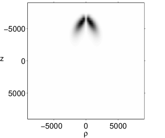
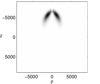
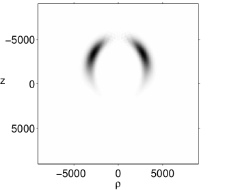
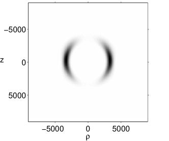
Figure 10: Manipulating the wavepacket by controlling the classical trajectory on which it is localized. Starting from the wavepacket depicted in the last frame of figure 7, the static field is turned off as described in the text. The plots show the electronic density obtained from a numerical resolution of the time-dependent Schrödinger equation. Top left $F_{s,0}=0.0027$, top right $F_{s,0}=0.00255$ (the wavepacket follows an elliptical trajectory), bottom left $F_{s,0}=0.00144$ (elliptical trajectory with low eccentricity) and bottom right $F_{s,0}=0$ - the circular trajectory.

Finally, when the static field is completely switched off, the square overlap with the desired Floquet state – a circular non-dispersive wavepacket – is slightly larger than 0.80. It proves that the scheme II that we propose is efficient although it involves several steps.

4 Conclusions

By numerical resolution of the time-dependent Schrödinger equation under realistic conditions and an analysis based on both semiclassical and exact numerical diagonalization of the Hamiltonian, we have shown how to prepare efficiently non-dispersive electronic wavepackets in the hydrogen atom which propagate either on a linear straight trajectory along the microwave field or on an elliptical trajectory of arbitrary eccentricity (the circular trajectory being the final state).

Although we concentrated on specific values of the field frequency and amplitude, the scheme is rather general and could be used for different parameters, with the following observations:

• For too low field amplitudes, the resonance island is so small that no well localized state actually exists. The rule of the thumb is that only $q$ values, see eq. (18), larger than unity should be used.

• For too large field values, the states are well localized, but ionize rather fast. Scaled microwave field amplitudes exceeding 0.04 are dangerous.

• Even if ionization remains small, it may happen for too large field values that the $n_{0}$ hydrogenic manifold is so large that it overlaps with neighboring $n_{0}\pm 1$ manifolds in the Floquet spectrum. This creates large avoided crossings which makes the adiabatic transfer impossible.

• For $n_{0}=60,$ the microwave frequency is 30 GHz and the total switching time if of the order of 120 ns. Such switching times should be feasible in a real experiment. Going to lower $n_{0}$ values would lead to higher frequency (and consequently more expensive microwave equipment) and shorter switching times. Going down to $n_{0}=30$ is thus rather a bad idea.

Excited wavepackets may be detected by employing short half-cycle pulses that lead to considerable ionization of the atom [22]. The ionization signal depends on the position of the center of the packet with respect to the nucleus at the moment when the pulse is applied (basically the ionization probability is larger the closer the center is situated with respect to the nucleus [22]). For a discussion of characteristic properties which would allow for an unambiguous characterization of the non-dispersive wavepackets, see [3].

5 Acknowledgment

Support of KBN under project 5P03B08821 (KS and JZ) is acknowledged. The additional support of the bilateral Polonium and PICS programs is appreciated. Laboratoire Kastler Brossel de l’Université Pierre et Marie Curie et de l’Ecole Normale Supérieure is UMR 8552 du CNRS. We thank IDRIS for providing us with CPU time on a NEC SX5 computer.

6 Appendix

In this appendix, we explain the semiclassical quantization procedure that allows us to obtain accurate predictions for the quasienergy levels and structures of the corresponding eigenstates of the atom in the presence of static and microwave external fields.

We begin with the effective Hamiltonian, Eq. (7). In the $(I,\hat{\theta})$ space, this Hamiltonian describes the motion in the vicinity of the fixed point at $I=n_{0}$. Expanding the Hamiltonian in powers of $\tilde{I}=I-n_{0}$ around the fixed point yields

$${\cal H}_{\mathrm{sec}}\approx\hat{P}_{t}-\frac{3}{2n_{0}^{2}}-\frac{3\tilde{I}^{2}}{2n_{0}^{4}}-\frac{3F_{s}n_{0}^{2}}{2}\sqrt{1-\frac{L^{2}}{n_{0}^{2}}}\cos\psi+F\Gamma(L,\psi)\cos[\hat{\theta}-\beta(L,\psi)].$$ (12)

The explicit expressions for $\Gamma$ and $\beta$ are as follows

$$\Gamma(L,\psi)=\sqrt{X_{1}^{2}\cos^{2}\psi+Y_{1}^{2}\sin^{2}\psi},$$ (13)

$$\tan\beta(L,\psi)=\frac{Y_{1}}{X_{1}}\tan\psi,$$ (14)

where

$$X_{1}(n_{0},L)=J^{\prime}_{1}(e)n_{0}^{2}$$ (15)

$$Y_{1}(n_{0},L)=\frac{L}{n_{0}e}J_{1}(e)n_{0}^{2}$$ (16)

with $e=\sqrt{1-L^{2}/n_{0}^{2}}$ being the eccentricity of the classical elliptical trajectory. $X_{1}$ and $Y_{1}$ are nothing but the oscillatory atomic dipoles in resonance with the external drive, along the major and minor axes of the classical Kepler ellipse, respectively.

As there is no explicit time dependence in eq. (12), the quantization of $\hat{P}_{t}$ is trivial [25, 27]. Taking into account that Floquet eigenstates have to be periodic in time, this yields $\hat{P}_{t}=k\omega$ (where $k$ is an integer number) which ensures the periodicity of the quasienergy spectrum with a period $\omega$.

The radial motion, i.e. in the $(\tilde{I},\hat{\theta})$ space, effectively decouples from the slow angular motion in the $(L,\psi)$ space [24]. In effect, one can quantize the system in the spirit of the Born-Oppenheimer approximation, i.e. first quantize the radial motion keeping the secular motion frozen [25, 27] and then switch to the quantization of the slow $(L,\psi)$ motion. The radial motion reveals a pendulum-like dynamics whose quantum eigenvalues are given by the solutions of the Mathieu equation [28]. As we are looking for solutions with maximum localization inside the resonance island, we will consider only the ground state solution of the pendulum (excited states of the pendulum describe the adjacent hydrogenic manifolds, see [27]). We obtain:

$${\cal H}_{\mathrm{eff}}=-\frac{3}{2n_{0}^{2}}-\frac{3}{8n_{0}^{4}}a_{0}(q)-\frac{3F_{s}n_{0}^{2}}{2}\sqrt{1-\frac{L^{2}}{n_{0}^{2}}}\cos\psi+k\omega,$$ (17)

where

$$q=\frac{4n_{0}^{4}F}{3}\Gamma(L,\psi)$$ (18)

is a dimensionless parameter. $a_{0}(q)$ is the Mathieu parameter corresponding to the ground state of the pendulum [28]. The last stage is to quantize the secular motion which can be done directly using the WKB rule [24, 27]

$$\frac{1}{2\pi}\oint Ld\psi=p+\frac{\mu}{4},$$ (19)

where $p$ is an integer number and $\mu$ stands for the Maslov index.

Without the static electric field, i.e. for $F_{s}=0$, it is more convenient to quantize the secular motion first (obtaining quantized values of $\Gamma$) and then switch to quantization in the $(\tilde{I},\hat{\theta})$ space. This is allowed because the entire dependence of the Hamiltonian on $L$ and $\psi$ is included in $\Gamma(L,\psi)$ [27]. In the presence of the static electric field, such a simplification is no longer possible and one has to use the whole Hamiltonian (17) to perform the semiclassical quantization in the $(L,\psi)$ space.

Although, for comparison of the semiclassical quasienergies with the quantum numerical values, we carry out calculations using the full Hamiltonian (17), it is instructive to perform further approximations and discuss weak and strong fields limit separately. For very small $F$ and moderate $n_{0}$, i.e. for $q\ll 1$, the Mathieu parameter can be approximated [28] by

$$a_{0}(q)\approx-\frac{q^{2}}{2}.$$ (20)

This is the regime corresponding to a very weak trapping pendulum potential, where the radial motion in the $(\tilde{I},\hat{\theta})$ space is basically the free motion slightly perturbed (at second order in $F$) by the potential. However even for negligible external fields, the character of the secular motion is changed completely. That is, for $F=0$ and $F_{s}=0,$ both $L$ and $\psi$ are conserved quantities (i.e. the shape and the orientation of the electronic ellipse remain unchanged) while for $F\neq 0$ or $F_{s}\neq 0,$ the motion in the $(L,\psi)$ phase space may reveal both librations (around a fixed point) and rotations as shown in Fig. 11. Contours in Fig. 11 correspond actually to the semiclassically quantized states according to the WKB prescription, eq. (19), for $n_{0}=60$. For fixed $F_{s}$ and with decreasing $F$, the fixed point on the $\psi=\pi$ axis moves from $L_{0}=L/n_{0}=1$ to $L_{0}=L/n_{0}=0$, see Fig. 11. This corresponds to an ellipse oriented along the field axis whose shape changes from a circle to a trajectory degenerated into a line. The eigenstate of the system with the contour situated in the vicinity of this fixed point possesses probability density localized around an ellipse whose eccentricity depends on $F/F_{s}$ ratio. However, there is no localization of an electron on such an elliptical trajectory because the pendulum island in the $(\tilde{I},\hat{\theta})$ space is too small to hold a semiclassical state — the density probability is equally distributed along the ellipse with a weak (periodic) time dependence.

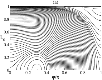
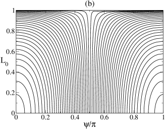
Figure 11: Structure of the $(L,\psi)$ phase space corresponding to the Hamiltonian (17) for $n_{0}=60$, $F_{s,0}=n_{0}^{4}F_{s}=10^{-6}$ and for $F_{0}=n_{0}^{4}F=10^{-4}$ [panel (a)], $F_{0}=n_{0}^{4}F=5\cdot 10^{-6}$ [panel (b)]. We use the scaled angular momentum $L_{0}=L/n_{0}$ in the plots. The ploted contours fulfill the semiclassical WKB quantization rule given by eq. (19).

In the opposite limit, i.e. for large $F$ or in the deep semiclassical limit $n_{0}\rightarrow\infty$, one may employ another asymptotic expression for the Mathieu parameter [28]

$$a_{0}(q)\approx-2|q|+2\sqrt{|q|}.$$ (21)

This corresponds to the case where the pendulum, in the $(\tilde{I},\hat{\theta})$ space, is localized near its stable equilibrium point. The equilibrium energy is $-2|q|$ while $2\sqrt{|q|}$ comes from the ground state energy of the pendulum calculated in the harmonic approximation. This is actually the approximation used in [24] where we have predicted the existence of nondispersive wavepackets in this system. The structure of the $(L,\psi)$ phase space has been presented in [24] and is very similar to that shown for the weak fields limit — e.g., there is also a fixed point located on the $\psi=\pi$ axis that changes its position when $F/F_{s}$ varies. The state in the vicinity of this fixed point corresponds to a well defined elliptical trajectory. However, in the present case, there is also localization of the electron on the trajectory because the island in the $(\tilde{I},\hat{\theta})$ space is large enough to support quantum eigenstates. This allows us to build the nondispersive wavepackets that are analyzed in the present article.

References

- [1] A. Bergou and B. G. Englert, J. Mod. Opt. 45, 701 (1998).
- [2] G. Alber and P. Zoller, Phys. Rep. 199, 231 (1991).
- [3] A. Buchleitner, D. Delande, and J. Zakrzewski, Phys. Rep. (2002) in press.
- [4] G. P. Berman and G. M. Zaslavsky, Phys. Lett. A 61, 295 (1977).
- [5] J. Henkel and M. Holthaus, Phys. Rev. A45, 1978 (1992).
- [6] M. Holthaus, Chaos, Solitons and Fractals 5, 1143 (1995).
- [7] D. Delande and A. Buchleitner, Adv. At. Mol. Opt. Phys. 35, 85 (1994).
- [8] A. Buchleitner and D. Delande, Phys. Rev. Lett. 75, 1487 (1995).
- [9] I. Bialynicki-Birula, M. Kaliński, and J. H. Eberly, Phys. Rev. Lett. 73, 1777 (1994).
- [10] D. Delande, J. Zakrzewski, and A. Buchleitner, Europhys. Lett. 32, 107 (1995).
- [11] J. Zakrzewski, D. Delande, and A. Buchleitner, Phys. Rev. Lett. 75, 4015 (1995).
- [12] J. H. Shirley, Phys. Rev. 138, B979 (1965).
- [13] J. Zakrzewski, D. Delande, and A. Buchleitner, Phys. Rev. E 57, 1458 (1998).
- [14] Z. Bialynicka-Birula and I. Bialynicki-Birula, Phys. Rev. A, 56, 3629 (1997).
- [15] D. Delande and J. Zakrzewski, Phys. Rev. A 58, 466 (1998).
- [16] K. Hornberger and A. Buchleitner, Europhys. Lett. 41, 383 (1998).
- [17] J. E. Bayfield, G. Casati, I. Guarneri, and D. W. Sokol, Phys. Rev. Lett. 63, 364 (1989).
- [18] E. J. Galvez et al., Phys. Rev. Lett. 61, 2011 (1988).
- [19] M. L. W. Bellermann, P. M. Koch, D. Mariani, and D. Richards, Phys. Rev. Lett. 76, 892 (1996).
- [20] M. W. Noël, M. W. Griffith, and T. F. Gallagher, Phys. Rev. A 62, 063401 (2000).
- [21] J. Zakrzewski and D. Delande, J. Phys. B 30, L87 (1997).
- [22] J. Bromage and C. R. Stroud, Jr., Phys. Rev. Lett. 83, 4963 (1999).
- [23] A. J. Lichtenberg and M. A. Liberman, Regular and Chaotic Dynamics, 2nd ed. Springer, New York, 1992.
- [24] K. Sacha, J. Zakrzewski and D. Delande, Europ. Phys. J. D, 1, 231 (1998).
- [25] K. Sacha, J. Zakrzewski, and D. Delande, Ann. Phys. 283, 141 (2000).
- [26] A. Buchleitner, D. Delande, and J. C. Gay, J. Opt. Soc. Am. B 12, 505 (1995).
- [27] A. Buchleitner, K. Sacha, D. Delande and J. Zakrzewski, Europ. Phys. J. D 5, 145 (1999).
- [28] in Handbook of Mathematical Functions, (M. Abrammowitz and I. A. Stegun Eds.) Dover, New York, 1972.