The classical limit for a class of quantum baker’s maps

Abstract

We show that the class of quantum baker’s maps defined by Schack and Caves have the proper classical limit provided the number of momentum bits approaches infinity. This is done by deriving a semi-classical approximation to the coherent-state propagator.

I Introduction

The introduction of ‘toy’ mappings which demonstrate essential features of nonlinear dynamics has led to many insights in the field of classical chaos. A well-known example is the so-called baker’s transformation Lichtenberg1992a . Interest in this mapping stems from its straightforward characterization in terms of a Bernoulli shift on binary sequences. It seems natural to consider a quantum counterpart to the baker’s map for the investigation of quantum chaos. Unfortunately, there is no unique quantization procedure, and hence, we must embrace the possibility of different quantum maps limiting to the same classical baker’s transformation.

Balazs and Voros Balazs1989a were first to conceive a quantum version of the baker’s map. This was done with the help of the discrete quantum Fourier transform. Subsequently, improvements to the Balazs-Voros quantization were made by Saraceno Saraceno1990a , an optical analogy was found hannay , a canonical quantization was devised Rubin1998a ; lesniewski , and quantum computing realizations have been proposed schack ; brun . A quantum baker’s mapping on the sphere has also been defined Pakonski1999a . More recently, an entire class of quantum baker’s maps was proposed by Schack and Caves using qubits Schack2000a . The Balazs-Voros quantization is but one member of this class.

The classical limit of the Schack-Caves quantizations is the subject of this article. We explicitly derive a semi-classical approximation for the propagator in the coherent state basis. This enables us to give conditions upon which the Schack-Caves quantizations will behave as the classical baker’s transformation in the limit $\hbar\rightarrow 0$. We find that, provided the number of momentum qubits approaches infinity, the semi-classical propagator takes the form

$$\langle b|\hat{B}|a\rangle\approx\sqrt{\frac{\partial^{2}W}{\partial a\partial b^{*}}}\exp\Big{[}W(b^{*},a)/2\hbar\Big{]}\exp\Big{[}-\big{(}|a|^{2}+|b|^{2}\big{)}/4\hbar\Big{]}$$

where $|a\rangle$ and $|b\rangle$ are coherent states on the torus, and $W(b^{*},a)$ is a classical generating function. Similar propagators have been encountered before using spin coherent states Kus1993a ; Scott2001a , but all may be thought of as variants of those derived long ago by Van Vleck Van1928a and Gutzwiller Gutzwiller1967a . Semi-classical propagators play an important role in the path-integral formulation of quantum mechanics Feynman and the related theory of periodic orbit quantization Brack . The latter has been investigated thoroughly for the Balazs-Voros quantum baker’s map ozorio ; eckhardt ; saraceno ; dittes ; laksh ; luz ; kaplan ; toscano ; tanner .

In deriving a semi-classical approximation only for the one-step propagator, we avoid complications which will arise after many iterations of the mapping. For long time scales, simple quantum-to-classical correspondences will break down inoue and one must incorporate the theories of decoherence Zurek ; Giulini ; Habib or continuous measurement Bhatt ; Scott2000a . The classical limit of the Schack-Caves quantization has already been investigated Soklakov2000a in this light using a decoherent histories approach Griffiths1984a ; Omnes1988a ; Gell1993a . However only a special case ($\theta=0$ in our notation) was considered. We proceed under an assumption that provided our one-step propagator agrees with the baker’s transformation in the semi-classical limit $\hbar\rightarrow 0$, decoherence will restore quantum-to-classical correspondences for long time scales.

The paper is organized as follows. In Section II, we introduce the baker’s map, both in classical and quantal form. Coherent states for a toroidal phase space are also introduced. In Section III our core results are presented. Here we derive semi-classical approximations to the coherent-state propagator and give conditions for when the Schack-Caves quantizations have the proper classical limit. Finally, in Section IV, we summarize our findings.

II A Class of Quantum Baker’s Maps

The baker’s map is a standard example in chaotic dynamics. It is a mapping of the unit square onto itself in the form

$$q_{n+1} = 2q_{n}-\lfloor 2q_{n}\rfloor$$ (1)

$$p_{n+1} = \left(p_{n}+\lfloor 2q_{n}\rfloor\right)/2$$ (2)

where $q,p\in[0,1)$, $\lfloor x\rfloor$ is the integer part of $x$, and $n$ denotes the $n$-th iteration of the map. Geometrically, the map stretches the unit square by a factor of two in the $q$ direction, squeezes by a factor of a half in the $p$ direction, and then stacks the right half onto the left.

The map’s action may be rewritten in terms of the complex variable $a\equiv q+ip$,

$$a_{n+1}^{\phantom{*}}=\frac{5}{4}a_{n}^{\phantom{*}}+\frac{3}{4}a_{n}^{*}+\left(\frac{i}{2}-1\right)\lfloor a_{n}^{\phantom{*}}+a_{n}^{*}\rfloor\equiv b_{n}^{\phantom{*}}(a_{n}^{\phantom{*}},a_{n}^{*}).$$ (3)

A generating function for this mapping (up to an arbitrary constant) is

$$W(b^{*},a)=\frac{1}{10}\left(3b^{*2}+8ab^{*}-3a^{2}\right)+\frac{4}{5}\left(1+\frac{i}{2}\right)\left(a+ib^{*}-\frac{1}{2}\right)\lfloor a+a^{*}\rfloor$$ (4)

assuming $a+a^{*}$ is non-integer. The classical baker’s map may then be rederived via the relations

$$\frac{\partial W}{\partial b^{*}}=b\qquad\qquad\frac{\partial W}{\partial a}=a^{*}.$$ (5)

Interest in the baker’s map is due mainly to the simplicity of its symbolic dynamics. If each point of the unit square is identified through its binary representation, $q=0\cdot s_{1}s_{2}\ldots=\sum_{k=1}^{\infty}s_{k}2^{-k}$ and $p=0\cdot s_{0}s_{-1}\ldots=\sum_{k=0}^{\infty}s_{-k}2^{-k-1}$ ($s_{i}\in\{0,1\}$), with a bi-infinite symbolic string

$$s=\ldots s_{-2}s_{-1}s_{0}\bullet s_{1}s_{2}s_{3}\ldots$$ (6)

then the action of the baker’s map is to shift the position of the dot by one point to the right,

$$s\rightarrow s^{\prime}=\ldots s_{-2}s_{-1}s_{0}s_{1}\bullet s_{2}s_{3}\ldots.$$ (7)

For a quantum mechanical version of the map, we work in the $D$-dimensional Hilbert space, ${\cal H}_{D}$, spanned by either the position states $|q_{j}\rangle$, with eigenvalues $q_{j}=(j+\beta)/D$, or momentum states $|p_{k}\rangle$, with eigenvalues $p_{k}=(k+\alpha)/D$ ($j,k=0\ldots D-1$). The constants $\alpha,\beta\in[0,1)$ determine the periodicity of the space: $|q_{j+D}\rangle=e^{-2\pi i\alpha}|q_{j}\rangle$, $|p_{k+D}\rangle=e^{2\pi i\beta}|p_{k}\rangle$. Such double periodicity identifies ${\cal H}_{D}$ with a toroidal phase space. The vectors of each basis are orthonormal $\langle q_{j}|q_{j^{\prime}}\rangle=\delta_{j,j^{\prime}}$, $\langle p_{k}|p_{k^{\prime}}\rangle=\delta_{k,k^{\prime}}$ and the two bases are related via the finite Fourier transform

$$\langle q_{j}|\hat{F}_{D}|q_{k}\rangle\equiv\langle q_{j}|p_{k}\rangle=\frac{1}{\sqrt{D}}e^{\frac{i}{\hbar}q_{j}p_{k}}.$$

For consistency of units, we must have $2\pi\hbar D=1$.

The first work on a quantum baker’s map was done by Balazs and Voros Balazs1989a . Their expression for the map was given in the form

$$\hat{B}=\hat{F}^{-1}_{D}\left(\begin{array}[]{cc}\hat{F}_{D/2}&0\\ 0&\hat{F}_{D/2}\end{array}\right)$$ (8)

where $\hat{F}_{D/2}$ is the finite Fourier transform acting on half of the Hilbert space. Later Saraceno Saraceno1990a improved certain symmetry characteristics of the map using anti-periodic boundary conditions ($\alpha=\beta=1/2$). Finally, taking again the anti-periodic Hilbert space, Schack and Caves Schack2000a introduced a whole class of quantum baker’s maps for dimensions $D=2^{N}$.

For these cases, we can model our space as the product of $N$ qubits with a binary expansion association

$$|q_{j}\rangle=|x_{1}\rangle\otimes|x_{2}\rangle\otimes\cdots\otimes|x_{N}\rangle\qquad x_{l}\in\{0,1\}$$ (9)

where $j$ has the binary expansion

$$j=x_{1}\ldots x_{N}\cdot 0=\sum_{l=1}^{N}x_{l}2^{N-l}\qquad\text{and}\qquad q_{j}=\frac{j+1/2}{D}.$$ (10)

Next we rewrite the quantum Fourier transform as

$$|p_{k}\rangle=\hat{F}_{D}|q_{k}\rangle=\frac{1}{\sqrt{2^{N}}}\sum_{x_{1},\ldots,x_{N}}|x_{1}\rangle\otimes|x_{2}\rangle\otimes\cdots\otimes|x_{N}\rangle\,e^{2\pi iyx/2^{N}}$$ (11)

where $y=y_{1}\ldots y_{N}\cdot 1=k+1/2$ and $x=x_{1}\ldots x_{N}\cdot 1=j+1/2$.

The connection with the classical baker’s map comes from its symbolic dynamics. In the quantum case, a string is created through the partial Fourier transform $\hat{G}_{n}$. It is an operator which Fourier transforms the $N-n$ least significant qubits of a state

$$\hat{G}_{n}\Big{(}|x_{1}\rangle\otimes\cdots\otimes|x_{n}\rangle\otimes|a_{1}\rangle\otimes\cdots\otimes|a_{N-n}\rangle\Big{)}\,\equiv\,|x_{1}\rangle\otimes\cdots\otimes|x_{n}\rangle\otimes\frac{1}{\sqrt{2^{N-n}}}\sum_{x_{n+1},\ldots,x_{N}}|x_{n+1}\rangle\otimes\cdots\otimes|x_{N}\rangle e^{2\pi iax/2^{N-n}}$$ (12)

where $a$ and $x$ are defined through the binary expansions $a=a_{1}\ldots a_{N-n}\cdot 1$ and $x=x_{n+1}\ldots x_{N}\cdot 1$. In the limiting cases, we have $\hat{G}_{0}=\hat{F}_{D}$ and $\hat{G}_{N}=i\hat{1}$.

The analogy to the classical case is made clear through the definition

$$|a_{N-n}\ldots a_{1}\bullet x_{1}\ldots x_{n}\rangle\equiv\hat{G}_{n}\Big{(}|x_{1}\rangle\otimes\cdots\otimes|x_{n}\rangle\otimes|a_{1}\rangle\otimes\cdots\otimes|a_{N-n}\rangle\Big{)}.$$ (13)

These states form an orthonormal basis and are localized in both position and momentum. They are strictly localized in a position region of width $1/2^{n}$ centered at $0\cdot x_{1}\ldots x_{n}1$, and are roughly localized in a momentum region of width $1/2^{N-n}$ centered at $0\cdot a_{1}\ldots a_{N-n}1$.

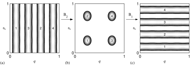
Figure 1: The Husimi function for each partially Fourier transformed state (13) when $N=2$, and, (a) $n=2$, (b) $n=1$ and (c) $n=0$.

Using this notation, Schack and Caves defined a whole class of quantum baker’s maps $\hat{B}_{n}$ ($n=1,\ldots,N$)

$$\hat{B}_{n}\,\equiv\,\hat{G}^{\phantom{-1}}_{n-1}\circ\hat{G}^{-1}_{n}\;=\sum_{\begin{array}[]{c}\scriptstyle x_{1},\dots,x_{n}\\ \scriptstyle a_{1},\dots,a_{N-n}\end{array}}|a_{N-n}\dots a_{1}x_{1}\bullet x_{2}\dots x_{n}\rangle\langle a_{N-n}\dots a_{1}\bullet x_{1}x_{2}\dots x_{n}|.$$ (14)

The Balazs-Voros-Saraceno quantum baker’s map is recovered when $n=1$. In the language of Eq. (6), we see that each quantum baker’s map takes a state localized at $1a_{N-n}\ldots a_{1}\bullet x_{1}\ldots x_{n}1$ to a state localized at $1a_{N-n}\ldots a_{1}x_{1}\bullet x_{2}\ldots x_{n}1$. The decrease in the number of position bits and increase in momentum bits enforces a stretching and squeezing of phase space in a manner resembling the classical baker’s map. In figures 1(a), (b) and (c), we have plotted the Husimi function (defined below) for the partially Fourier transformed states (13) when $N=2$, and $n=2$, 1 and 0, respectively. The quantum baker’s map is simply a one-to-one mapping of one basis to another.

It will be useful to rewrite our baker’s map in the position basis. To do this, we first use (12) and (13) to rewrite Eq. (14) as

$$\hat{B}_{n} = \frac{\sqrt{2}}{2^{N-n+1}}\sum_{\begin{array}[]{c}\scriptstyle x_{1},\dots,x_{n}\\ \scriptstyle a_{1},\dots,a_{N-n}\end{array}}\sum_{\begin{array}[]{c}\scriptstyle z_{1},\dots,z_{N-n+1}\\ \scriptstyle y_{1},\dots,y_{N-n}\end{array}}|\bullet x_{2}\dots x_{n}z_{1}\dots z_{N-n+1}\rangle\langle\,\bullet\,x_{1}\dots x_{n}y_{1}\dots y_{N-n}|$$

$$\qquad\times\exp\left[\frac{\pi i}{2^{N-n}}\Big{(}(j+1/2)(l+1/2)+2^{N-n}x_{1}(l+1/2)-2(j+1/2)(k+1/2)\Big{)}\right]$$

where

$$j=\sum_{k=1}^{N-n}a_{k}2^{N-n-k}\text{,}\quad k=\sum_{k=1}^{N-n}y_{k}2^{N-n-k}\quad\text{and}\quad l=\sum_{k=1}^{N-n+1}z_{k}2^{N-n+1-k}.$$

Next, using (9), (13) and the notation $q_{j}=(j+1/2)/D$, $q_{k}=(k+1/2)/D$, etc, we arrive at the quantum baker’s map in the position basis

$$\hat{B}_{n} = \frac{\sqrt{2}}{2^{N-n+1}}\>\>\sum_{x_{1}=0}^{1}\>\>\>\sum_{j,k=0}^{2^{N-n}-1}\>\>\>\sum_{l=0}^{2^{N-n+1}-1}\>\>\>\sum_{m=0}^{2^{n-1}-1}$$ (20)

$$\qquad\times\quad\Big{|}q_{l}+q_{m}2^{N-n+1}-2^{-n}\Big{\rangle}\Big{\langle}q_{k}+x_{1}/2+q_{m}2^{N-n}-2^{-n-1}\Big{|}$$

$$\qquad\qquad\times\quad\exp\left[i\pi D2^{n}\left(q_{j}q_{l}+2^{-n}x_{1}q_{l}-2q_{j}q_{k}\right)\right].$$

Note that it is possible to sum over the index $j$ at this point. However the above representation proves to be most convenient when performing our semi-classical analysis.

We will now introduce coherent states for ${\cal H}_{D}$ Jin1985a ; Leboeuf1990a ; Nonnenmacher1998a :

$$|a\rangle \equiv \frac{1}{\cal N}\left(\frac{2}{D}\right)^{1/4}\sum_{\mu=-\infty}^{\infty}\sum_{j=0}^{D-1}\exp\left[-\frac{\pi D}{2}\left(|a|^{2}-a^{2}\right)-\pi D\left(q_{j}-a+\mu\right)^{2}+i\pi\mu\right]|q_{j}\rangle$$ (21)

$$= \frac{1}{\cal N}\left(\frac{2}{D}\right)^{1/4}\;\sum_{j=0}^{D-1}\exp\left[-\frac{\pi D}{2}\left(|a|^{2}+a^{2}\right)-\pi D\left(q_{j}^{2}-2q_{j}a\right)\right]\theta_{0}\big{[}iD(q_{j}-a)\big{|}iD\big{]}|q_{j}\rangle$$ (22)

where $a\equiv q+ip$ and $\theta_{0}$ is called a theta function akhiezer

$$\theta_{0}\big{[}z\big{|}\tau\big{]}\equiv\sum_{\mu=-\infty}^{\infty}\exp\big{[}i\pi\big{(}\tau\mu^{2}+(2z+1)\mu\big{)}\big{]}.$$ (23)

The coherent states obey $|a\pm 1\rangle=-\exp[\pm\pi iDp]|a\rangle$, $|a\pm i\,\rangle=-\exp[\mp\pi iDq]|a\rangle$, and are simply the standard (Weyl group) coherent states that have been (anti-) periodicized and then projected onto ${\cal H}_{D}$. The normalization factor takes the form

$${\cal N}^{2}=\theta_{0}\big{[}qD\big{|}iD/2\big{]}\theta_{0}\big{[}pD\big{|}iD/2\big{]}=1+O(1/D)\qquad(D\text{ even})$$ (24)

and henceforth, will be set to unity. Finally, the Husimi function for our toroidal phase space is defined as $|\langle\psi|a\rangle|^{2}$.

III The Semi-Classical Propagator

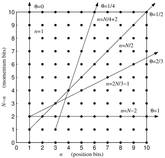
Our goal in this section is to explicitly calculate the semi-classical propagator in the coherent state basis. That is, we wish to obtain the leading term in an asymptotic expansion of the matrix element $\langle b|\hat{B}_{n}|a\rangle$ as $D\rightarrow\infty$. Observe from Eq. (14) that in this limit, the total number of position and momentum bits $N$ necessarily become infinite. However one has considerable freedom of choice on how this may occur (see Fig. 2). We wish to consider cases where the relative number of position and momentum bits approach infinity at different rates. To this end, we take the number of position bits to be in the explicit form $n=n(N)\equiv\theta N+s$, where $0\leq\theta\leq 1$ is rational and $s$ takes integer values. For ease of reading, we also introduce the constant $\phi=1-\theta$ such that the number of momentum bits $N-n=\phi N-s$. We will also now identify the different quantum baker’s maps through the new parameters, $\hat{B}_{\theta,s}\equiv\hat{B}_{n}$. The parameter $\theta$ ($\phi$) may be interpreted as the fraction of qubits allocated to the position (momentum) register as the total number of qubits $N$, is increased. In the analysis which follows we must consider the two cases $\theta=0$ and $\theta=1$ separately. The former contains the original Balazs-Voros-Saraceno quantization ($n=s=1$) and will be investigated first. The second parameter $s$, describes an initial offset between the number of position and momentum qubits and has no semi-classical effect when $\theta<1$. We will find, however, that $s$ becomes important when $\theta=1$.

Figure 2: Different possible ways of taking the classical limit for the quantum baker’s map.

III.1 Case $\theta=0$.

In this case the number of position bits remains constant $n=s\geq 1$ as we let $D\rightarrow\infty$. Using (20) and (21) our matrix element becomes

$$\langle b|\hat{B}_{0,s}|a\rangle = SD^{-3/2}\>\sum_{\mu,\nu=-\infty}^{\infty}\>\>\>\sum_{x_{1}=0}^{1}\>\>\>\sum_{j,k=0}^{D/S-1}\>\>\>\sum_{l=0}^{2D/S-1}\>\>\>\sum_{m=0}^{S/2-1}\>\>\>$$ (25)

$$\exp\bigg{[}-\frac{\pi D}{2}\Big{(}|a|^{2}+|b|^{2}-a^{2}-b^{*2}\Big{)}+i\pi(\mu-\nu)-\pi D\Big{(}q_{k}+x_{1}/2+(Dq_{m}-1/2)/S-a+\mu\Big{)}^{2}$$

$$-\;\pi D\Big{(}q_{l}+2(Dq_{m}-1/2)/S-b^{*}+\nu\Big{)}^{2}+i\pi SD\Big{(}q_{j}q_{l}+x_{1}q_{l}/S-2q_{j}q_{k}\Big{)}\bigg{]}$$

where $S\equiv 2^{s}$. To further the calculation, we now use variants of the Poisson summation formula to replace each sum with $D$ in the upper limit, by an integral e.g.

$$\sum_{\alpha=-\infty}^{\infty}\int_{0}^{1/S}\exp\Big{[}2\pi i(Dx-1/2)\alpha\Big{]}f(x)dx=\frac{1}{D}\int_{0}^{1/S}\sum_{j=-\infty}^{\infty}\delta\Big{(}x-(j+1/2)/D\Big{)}f(x)dx=\frac{1}{D}\sum_{j=0}^{D/S-1}f(q_{j}).$$ (26)

The result is

$$\langle b|\hat{B}_{0,s}|a\rangle = SD^{3/2}\mathop{\sum_{\mu,\nu,\alpha}^{\infty}}_{\beta,\gamma=-\infty}\>\>\>\sum_{x_{1}=0}^{1}\>\>\>\sum_{m=0}^{S/2-1}\>\>\>\int_{0}^{1/S}dx\int_{0}^{1/S}dy\int_{0}^{2/S}dz$$ (27)

$$\exp\bigg{[}-\frac{\pi D}{2}\Big{(}|a|^{2}+|b|^{2}-a^{2}-b^{*2}\Big{)}+i\pi(\mu-\nu-\alpha-\beta-\gamma)$$

$$-\;\pi D\Big{(}y+x_{1}/2+m/S-a+\mu\Big{)}^{2}-\pi D\Big{(}z+2m/S-b^{*}+\nu\Big{)}^{2}$$

$$+\;i\pi SD\Big{(}xz+x_{1}z/S-2xy\Big{)}+2i\pi D\left(x\alpha+y\beta+z\gamma\right)\bigg{]}.$$

We are now ready to make a semi-classical approximation to our matrix element. More precisely, we will make a saddle-point approximation to the triple integral above. Only near a saddle-point will contributions from such an integral cancel the prefactor $D^{3/2}$ and lead to an $O(1)$ contribution for the matrix element. The saddle-point approximation can be written down immediately using well-known formulae found in any standard text wong . However the limits in the above integrals are finite; therefore, the saddle point will not make a contribution in all cases. We need to consider this possibility carefully if we are to recover the classical baker’s map. Hence, we will treat each one-dimensional integral separately and use the method of steepest descents.

Consider first the $y$ integration (with $x$ a parameter) by defining

$$I_{1}\equiv\int_{0}^{1/S}dy\>\exp\big{[}-\pi Df(y)\big{]}$$ (28)

where

$$f(y) \equiv (y-A)^{2}+2i(Sx-\beta)y$$ (29)

$$A \equiv a-x_{1}/2-m/S-\mu.$$ (30)

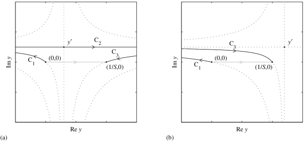
Figure 3: Steepest descent paths for $f(y)$. The original integration path along the real line (gray) is deformed to one where $\,\text{Im}\,f(y)=\text{constant}$ (black).

An asymptotic calculation of this integral is enabled by deforming the integration path, currently along the real line, to one in the complex plane where $\,\text{Im}\,f(y)=\text{constant}$. Two important cases are drawn in Fig. 3. The first (a) occurs when the saddle point (defined through $f^{\prime}(y^{\prime})=0$)

$$y^{\prime}=A-iSx+i\beta$$ (31)

satisfies $0<\,\text{Re}\,y^{\prime}<1/S$. In this case, the steepest descent path is one which first travels along the hyperbola $C_{1}$ from $0$ to $-\infty+i\,\text{Im}\,y^{\prime}$, then along the hyperbolic asymptote $C_{2}$ to $\infty+i\,\text{Im}\,y^{\prime}$, and finally back to $1/S$ via another hyperbola $C_{3}$. Hence an asymptotic expansion for the integral $I_{1}$ will be the sum of three parts, each associated with a different contour $C_{1}$, $C_{2}$ or $C_{3}$ in the complex plane. Note that along the contours $C_{1}$ and $C_{3}$, the kernel attains its maximum at the end points $0$ and $1/S$, respectively. Consequently, the leading term in an asymptotic expansion takes the form

$$\frac{-1}{\pi Df^{\prime}(c)}\exp\big{[}-\pi Df(c)\big{]}\big{[}1+O(1/D)\big{]}$$ (32)

with $c=0$ or $1/S$. However the prefactor of $1/D$ in the above inhibits such terms from playing a role in the leading order approximation of our matrix element. As remarked before, we need prefactors of $D^{-1/2}$ in each approximation of the three integrals in (27) in order to obtain an $O(1)$ overall contribution for the matrix element. Hence we will simply discard the integration along contours $C_{1}$ and $C_{3}$, and make the approximation

$$I_{1} \approx \int_{-\infty+i\,\text{Im}\,y^{\prime}}^{\infty+i\,\text{Im}\,y^{\prime}}dy\>\exp\big{[}-\pi Df(y)\big{]}\qquad\text{if}\qquad 0<\,\text{Re}\,y^{\prime}<1/S$$ (33)

$$= D^{-1/2}\exp\big{[}-\pi Df(y^{\prime})\big{]}.$$ (34)

When $\,\text{Re}\,y^{\prime}<0$ or $\,\text{Re}\,y^{\prime}>1/S$ (Fig. 3(b)) the path of steepest descent no longer passes through the saddle point, and consequently, there will be no leading order contributions to the matrix element, i.e. we may set $I_{1}=0$. The third and final case occurs when $\,\text{Re}\,y^{\prime}=0$ or $1/S$. One may investigate these possibilities by taking exactly one half of (34) as the approximation for $I_{1}$. However, for simplicity, we will not deal with this case, except make the odd casual remark when needed. In summary, we take (34) as our approximation for $I_{1}$ when $0<\,\text{Re}\,y^{\prime}<1/S$, and otherwise zero.

Similarly, for the $z$ integration one has

$$I_{2} \equiv \int_{0}^{2/S}dz\>\exp\big{[}-\pi Dg(z)\big{]}$$ (35)

$$\approx D^{-1/2}\exp\big{[}-\pi Dg(z^{\prime})\big{]}\qquad\text{if}\qquad 0<\,\text{Re}\,z^{\prime}<2/S$$ (36)

with

$$g(z) \equiv (z-B)^{2}-2i(Sx/2+x_{1}/2+\gamma)z$$ (37)

$$B \equiv b^{*}-2m/S-\nu$$ (38)

and the saddle point is

$$z^{\prime}=B+iSx/2+ix_{1}/2+i\gamma.$$ (39)

Now letting $x$ vary again and setting

$$h(x) \equiv f(y^{\prime})+g(z^{\prime})-2i\alpha x$$ (40)

$$= \frac{5}{4}S^{2}x^{2}+S\Big{(}2iA-iB+x_{1}/2-2\beta+\gamma-2i\alpha/S\Big{)}x-2iA\beta-iB(x_{1}+2\gamma)+\beta^{2}+(x_{1}/2+\gamma)^{2}$$ (41)

we have the final integral

$$I_{3} \equiv \int_{0}^{1/S}dx\>\exp\big{[}-\pi Dh(x)\big{]}$$ (42)

$$\approx \sqrt{\frac{4}{5S^{2}D}}\exp\big{[}-\pi Dh(x^{\prime})\big{]}\qquad\text{if}\qquad 0<\,\text{Re}\,x^{\prime}<1/S$$ (43)

with the saddle point at

$$x^{\prime}=-\frac{2}{5S}\Big{(}2iA-iB+x_{1}/2-2\beta+\gamma-2i\alpha/S\Big{)}.$$ (44)

Now, inserting our saddle-point approximations back into (27) and setting $a\equiv a_{1}+ia_{2}$ and $b\equiv b_{1}+ib_{2}$, with a little algebra we obtain

$$\langle b|\hat{B}_{0,s}|a\rangle \approx \sqrt{\frac{4}{5}}\mathop{\sum_{\mu,\nu,\alpha}^{\infty}}_{\beta,\gamma=-\infty}\>\sum_{x_{1}=0}^{1}\>\>\sum_{m=0}^{S/2-1}\>\>\exp\bigg{[}-\frac{\pi D}{5}\Big{\{}(2a_{1}-b_{1}-x_{1}-2\mu+\nu-2\alpha/S)^{2}$$ (45)

$$+\;(a_{2}-2b_{2}+x_{1}+\beta+2\gamma)^{2}\Big{\}}+i\pi(\mu-\nu-\alpha-\beta-\gamma)+i\pi D(a_{1}a_{2}-b_{1}b_{2})$$

$$-\;\frac{2i\pi D}{5}\Big{\{}(2a_{1}-b_{1}-x_{1}-2\mu+\nu-2\alpha/S)(2a_{2}+b_{2})$$

$$-\;(a_{1}+2b_{1}-x_{1}/2-\mu-2\nu)(x_{1}+\beta+2\gamma)+\alpha(x_{1}-4\beta+2\gamma)/S\Big{\}}\bigg{]}$$

provided that all three of the inequalities

$$0 < \,\text{Re}\,x^{\prime}=\frac{2}{5S}\Big{(}2a_{2}+b_{2}-x_{1}/2+2\beta-\gamma\Big{)}<\frac{1}{S}$$ (46)

$$0 < \,\text{Re}\,y^{\prime}=\frac{1}{5}\Big{(}a_{1}+2b_{1}-x_{1}/2-\mu-2\nu\Big{)}+\frac{1}{5S}\Big{(}4\alpha-5m\Big{)}<\frac{1}{S}$$ (47)

$$0 < \frac{1}{2}\,\text{Re}\,z^{\prime}=\frac{1}{5}\Big{(}a_{1}+2b_{1}-x_{1}/2-\mu-2\nu\Big{)}-\frac{1}{5S}\Big{(}\alpha+5m\Big{)}<\frac{1}{S}$$ (48)

are satisfied. Otherwise the summand is taken to be zero.

Note that although $m$ no longer appears in the exponent, we cannot trivially evaluate the sum since not all values of $m$ will satisfy (47) and (48). Consider the cases when the approximation (45) becomes $O(1)$. That is,

$$2a_{1}-b_{1}-x_{1}-2\mu+\nu-2\alpha/S = 0$$ (49)

$$a_{2}-2b_{2}+x_{1}+\beta+2\gamma = 0.$$ (50)

Substituting (50) into (46) we obtain

$$0<a_{2}+\beta<1\qquad\text{or}\qquad 0<b_{2}-x_{1}/2-\gamma<1/2$$ (51)

and thus, the integers $\beta$ and $\gamma$ give our periodicity in the momentum direction. Hence if we assume $0<a_{2},b_{2}<1$ then we may set $\beta=\gamma=0$ in (45), making note that we are discarding exponentially small Gaussian tails. Also note from (51) that we must have $x_{1}=\lfloor 2b_{2}\rfloor$.

Now, negating (48) and adding it to (47) we immediately arrive at the inequality $-1<\alpha<1$. Hence we must set $\alpha=0$. This implies

$$\frac{2m}{S}<\frac{2}{5}\Big{(}a_{1}+2b_{1}-x_{1}/2-\mu-2\nu\Big{)}<\frac{2(m+1)}{S}$$ (52)

from (47,48), or equivalently

$$0<\frac{2}{5}\Big{(}a_{1}+2b_{1}-x_{1}/2-\mu-2\nu\Big{)}<1$$ (53)

if we now drop the summation over $m$ in (45). Hence, following a similar procedure to the above, one can substitute (49) into the new inequality (53) and deduce that under the assumption $0<a_{1},b_{1}<1$, the summand of (45) becomes $O(1)$ only when $\mu=\nu=0$. Furthermore, we will have $x_{1}=\lfloor 2a_{1}\rfloor$.

The surviving term of the summation is our semi-classical approximation for the propagator:

$$\langle b|\hat{B}_{0,s}|a\rangle = \sqrt{\frac{4}{5}}\exp\bigg{[}-\frac{\pi D}{5}\Big{\{}\big{(}2a_{1}-b_{1}-\lfloor 2a_{1}\rfloor\big{)}^{2}+\big{(}a_{2}-2b_{2}+\lfloor 2a_{1}\rfloor\big{)}^{2}$$ (54)

$$+\;i\big{(}3a_{1}a_{2}+3b_{1}b_{2}+4a_{1}b_{2}-4a_{2}b_{1}\big{)}-2i\lfloor 2a_{1}\rfloor\big{(}a_{1}+2b_{1}+2a_{2}+b_{2}-\lfloor 2a_{1}\rfloor/2\big{)}\Big{\}}\bigg{]}+o(1)$$

where we have chosen $x_{1}=\lfloor 2a_{1}\rfloor$ (and implicitly assumed $a_{1}\neq 1/2$ and $b_{2}\neq 1/2$ by ignoring cases of equality in (46-48)). All other terms in (45), being exponentially small, are discarded.

Note that the above approximation is $O(1)$ only when $b$ is the iterate of $a$ under the classical baker’s map (3). Furthermore, a little algebra reveals that our semi-classical propagator may be rewritten in the Van Vleck form

$$\langle b|\hat{B}_{0,s}|a\rangle=\sqrt{\frac{\partial^{2}W}{\partial a\partial b^{*}}}\exp\Big{[}\pi DW(b^{*},a)\Big{]}\exp\Big{[}-\pi D\left(|a|^{2}+|b|^{2}\right)/2\Big{]}+o(1)$$ (55)

where $W(b^{*},a)$ is the classical generating function (4). Hence we have shown that the class of quantum baker’s map with $\theta=0$ will approach the classical baker’s map in the limit $D\rightarrow\infty$.

III.2 Case $0<\theta<1$.

We will now consider the case $0<\theta<1$. Using (20) and (21) with $n=\theta N+s$, our matrix element is

$$\langle b|\hat{B}_{\theta,s}|a\rangle = \frac{S}{\sqrt{D}D^{\phi}}\>\sum_{\mu,\nu=-\infty}^{\infty}\>\>\>\sum_{x_{1}=0}^{1}\>\>\>\sum_{j,k=0}^{D^{\phi}/S-1}\>\>\>\sum_{l=0}^{2D^{\phi}/S-1}\>\>\>\sum_{m=0}^{SD^{\theta}/2-1}\>\>\>$$ (56)

$$\exp\bigg{[}-\frac{\pi D}{2}\Big{(}|a|^{2}+|b|^{2}-a^{2}-b^{*2}\Big{)}+i\pi(\mu-\nu)-\pi D\Big{(}\big{(}q^{\phi}_{k}-1/2S\big{)}/D^{\theta}+x_{1}/2+q^{\theta}_{m}/S-a+\mu\Big{)}^{2}$$

$$-\;\pi D\Big{(}\big{(}q^{\phi}_{l}-1/S\big{)}/D^{\theta}+2q^{\theta}_{m}/S-b^{*}+\nu\Big{)}^{2}+i\pi SD^{\phi}\Big{(}q^{\phi}_{j}q^{\phi}_{l}+x_{1}q^{\phi}_{l}/S-2q^{\phi}_{j}q^{\phi}_{k}\Big{)}\bigg{]}$$

where again $S\equiv 2^{s}$. Introducing the new summing variables $q^{\theta}_{m}\equiv q_{m}D/D^{\theta}$, $q^{\phi}_{j}\equiv q_{j}D/D^{\phi}$, etc., enables us to convert the four finite sums over $j$, $k$, $l$ and $m$, to integrals over $x$, $y$, $z$ and $t$, respectively, using formulae similar to (26). The result is

$$\langle b|\hat{B}_{\theta,s}|a\rangle = S\sqrt{D}D^{\phi}\>\mathop{\sum_{\mu,\nu,\alpha,\beta}^{\infty}}_{\gamma,\kappa=-\infty}\>\>\>\sum_{x_{1}=0}^{1}\>\>\>\int_{0}^{1/S}dx\int_{0}^{1/S}dy\int_{0}^{2/S}dz\int_{0}^{S/2}dt$$ (58)

$$\exp\bigg{[}-\frac{\pi D}{2}\Big{(}|a|^{2}+|b|^{2}-a^{2}-b^{*2}\Big{)}+i\pi(\mu-\nu-\alpha-\beta-\gamma-\kappa)$$

$$-\;\pi D\Big{(}\big{(}y-1/2S\big{)}/D^{\theta}+x_{1}/2+t/S-a+\mu\Big{)}^{2}-\pi D\Big{(}\big{(}z-1/S\big{)}/D^{\theta}+2t/S-b^{*}+\nu\Big{)}^{2}$$

$$+\;i\pi SD^{\phi}\Big{(}xz+x_{1}z/S-2xy\Big{)}+2i\pi D^{\phi}(x\alpha+y\beta+z\gamma)+2i\pi D^{\theta}t\kappa\bigg{]}$$

$$= \frac{\sqrt{D}D^{\phi}}{S}\>\mathop{\sum_{\mu,\nu,\alpha,\beta}^{\infty}}_{\gamma,\kappa=-\infty}\>\>\>\sum_{x_{1}=0}^{1}\>\>\>\int_{0}^{1}dx\int_{0}^{1}dy\int_{0}^{2}dz\int_{0}^{1/2}dt$$

$$\exp\bigg{[}-\frac{\pi D}{2}\Big{(}|a|^{2}+|b|^{2}-a^{2}-b^{*2}\Big{)}+i\pi(\mu-\nu-\alpha-\beta-\gamma-\kappa)$$

$$-\;\pi D\big{(}t+x_{1}/2-a+\mu\big{)}^{2}-\pi D\big{(}2t-b^{*}+\nu\big{)}^{2}$$

$$-\;2\pi D^{\phi}\big{(}y-1/2\big{)}\big{(}t+x_{1}/2-a+\mu\big{)}/S-2\pi D^{\phi}\big{(}z-1\big{)}\big{(}2t-b^{*}+\nu\big{)}/S$$

$$+\;i\pi D^{\phi}\big{(}xz+x_{1}z-2xy\big{)}/S+2i\pi D^{\phi}\big{(}x\alpha+y\beta+z\gamma\big{)}/S$$

$$-\;\pi D^{\phi-\theta}\big{(}y-1/2\big{)}^{2}/S^{2}-\pi D^{\phi-\theta}\big{(}z-1\big{)}^{2}/S^{2}+2i\pi SD^{\theta}t\kappa\bigg{]}$$

where we have rescaled the integration variables ($x\rightarrow x/S$, $y\rightarrow y/S$, $z\rightarrow z/S$ and $t\rightarrow tS$), then collected terms in the exponent with the same power of $D$. The terms with highest power are those containing $t$, and hence, we will consider the integration over this variable first. Define the integral

$$I_{4}\equiv\int_{0}^{1/2}dt\>\exp\Big{[}-\pi D(t-A)^{2}-\pi D(2t-B)^{2}-2\pi D^{\phi}tC+2i\pi SD^{\theta}t\kappa\Big{]}$$ (59)

where the constants are

$$A \equiv a-x_{1}/2-\mu$$ (60)

$$B \equiv b^{*}-\nu$$ (61)

$$C \equiv (y-1/2)/S+2(z-1)/S.$$ (62)

We now wish to derive the contribution from $I_{4}$ which gives the leading order approximation to our matrix element. This is done by taking a path of steepest descent for the function $f(t)\equiv(t-A)^{2}+(2t-B)^{2}$. Note that when $\phi=1$ the third term of the exponent in (59) also becomes dominant and must be incorporated into $f(t)$. Hence the need to consider this case separately in the previous section.

As before, we may discard all parts of our integration contour, except the segment $(-\infty+i\,\text{Im}\,t^{\prime},\infty+i\,\text{Im}\,t^{\prime})$ which passes through the saddle point

$$t^{\prime}=\frac{A+2B}{5}.$$ (63)

It is only this contribution which will cancel the prefactor $\sqrt{D}D^{\phi}$ in (58) to give an $O(1)$ overall contribution to the matrix element. Hence we make the approximation

$$I_{4} \approx \int_{-\infty+i\,\text{Im}\,t^{\prime}}^{\infty+i\,\text{Im}\,t^{\prime}}dt\>\exp\Big{[}-\pi D(t-A)^{2}-\pi D(2t-B)^{2}-2\pi D^{\phi}tC+2i\pi SD^{\theta}t\kappa\Big{]}$$ (65)

$$= \frac{1}{\sqrt{5D}}\exp\bigg{[}-\frac{\pi D}{5}(2A-B)^{2}-\frac{2\pi D^{\phi}}{5}(A+2B)C+\frac{2i\pi D^{\theta}}{5}(A+2B)S\kappa$$

$$+\;\frac{\pi D^{\phi-\theta}}{5}C^{2}-\frac{\pi D^{\theta-\phi}}{5}S^{2}\kappa^{2}-\frac{2i\pi}{5}CS\kappa\bigg{]}$$

if $0<\,\text{Re}\,t^{\prime}<1/2$, and otherwise zero.

Substituting this approximation back into (58) and simplifying we obtain

$$\langle b|\hat{B}_{\theta,s}|a\rangle \approx \frac{D^{\phi}}{\sqrt{5}S}\>\mathop{\sum_{\mu,\nu,\alpha,\beta}^{\infty}}_{\gamma,\kappa=-\infty}\>\>\>\sum_{x_{1}=0}^{1}\>\>\>\int_{0}^{1}dx\int_{0}^{1}dy\int_{0}^{2}dz$$ (66)

$$\exp\bigg{[}-\frac{\pi D}{2}\Big{(}|a|^{2}+|b|^{2}-a^{2}-b^{*2}\Big{)}+i\pi(\mu-\nu-\alpha-\beta-\gamma)-\frac{\pi D}{5}\big{(}2A-B\big{)}^{2}$$

$$+\;\frac{2\pi D^{\phi}}{5S}\big{(}2A-B\big{)}\big{(}2y-z\big{)}+\frac{i\pi D^{\phi}}{S}\big{(}xz+x_{1}z-2xy\big{)}+\frac{2i\pi D^{\phi}}{S}\big{(}x\alpha+y\beta+z\gamma\big{)}$$

$$-\;\frac{\pi D^{\phi-\theta}}{5S^{2}}\big{(}2y-z\big{)}^{2}-\frac{2i\pi}{5}\big{(}y+2z\big{)}\kappa+\frac{2i\pi D^{\theta}}{5}\big{(}A+2B\big{)}S\kappa-\frac{\pi D^{\theta-\phi}}{5}S^{2}\kappa^{2}\bigg{]}.$$

The dominant terms in the exponent which contain the integration variables, are now those with $D^{\phi}$ as a prefactor. These terms do not define a saddle point, but instead, a line. Hence, it is advantageous to first decouple $x$, $y$ and $z$ in these terms using the following transformation

$$\left[\begin{array}[]{l}u\\ v\\ w\end{array}\right]=\left[\begin{array}[]{rrr}1&-2&1\\ 1&2&-1\\ 0&1&2\end{array}\right]\left[\begin{array}[]{l}x\\ y\\ z\end{array}\right]$$ (67)

where the integration region $(x,y,z)\in[0,1]\times[0,1]\times[0,2]$ is transformed to some parallel-piped $\Omega$.

After making this transformation, Eq. (66) may be rewritten in the form

$$\langle b|\hat{B}_{\theta,s}|a\rangle\approx\frac{D^{\phi}}{10\sqrt{5}S}\mathop{\sum_{\mu,\nu,\alpha,\beta}^{\infty}}_{\gamma,\kappa=-\infty}\>\>\sum_{x_{1}=0}^{1}\>\>\mathop{\int\!\!\!\!\int\!\!\!\!\int}_{\Omega}du\,dv\,dw\,\exp\bigg{[}-\frac{\pi D^{\phi}}{S}g(u)-\frac{\pi D^{\phi}}{S}h(v)-\frac{\pi D^{\phi-\theta}}{20S^{2}}(u-v)^{2}\bigg{]}F(w)$$ (68)

where

$$g(u) \equiv -\frac{i}{4}u^{2}-(E+i\alpha)u$$ (69)

$$h(v) \equiv \frac{i}{4}v^{2}+(E-i\alpha)v$$ (70)

$$E \equiv -\frac{1}{5}\big{(}2A-B\big{)}+\frac{i}{5}\big{(}x_{1}/2-2\beta+\gamma\big{)}\equiv E_{1}+iE_{2}$$ (71)

and

$$F(w) \equiv \exp\bigg{[}-\frac{\pi D}{2}\Big{(}|a|^{2}+|b|^{2}-a^{2}-b^{*2}\Big{)}+i\pi(\mu-\nu-\alpha-\beta-\gamma)-\frac{\pi D}{5}\big{(}2A-B\big{)}^{2}$$ (72)

$$+\;\frac{2i\pi D^{\theta}}{5}\big{(}A+2B\big{)}S\kappa-\frac{\pi D^{\theta-\phi}}{5}S^{2}\kappa^{2}+\frac{2i\pi}{5S}\Big{(}D^{\phi}(x_{1}+\beta+2\gamma)-S\kappa\Big{)}w\bigg{]}.$$

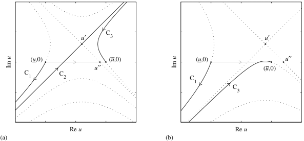
Figure 4: Steepest descent paths for $g(u)$.

We have now arrived at a form where we can consider steepest descent paths for the integration variables $u$ and $v$. Starting our program with the function $g(u)$ and writing $u$ in terms of its real and imaginary parts $u=u_{1}+iu_{2}$, ones finds that the two hyperbolic asymptotes

$$u_{1}-u^{\prime}_{1} = u_{2}-u^{\prime}_{2}$$ (73)

$$u_{1}-u^{\prime}_{1} = -u_{2}+u^{\prime}_{2}$$ (74)

are the steepest descent paths which pass through the saddle point

$$u^{\prime}=u_{1}^{\prime}+iu_{2}^{\prime}=2(iE-\alpha).$$ (75)

However, only the first (73) can be used as an integration contour, since $\exp\left[-\pi D^{\phi}\,\text{Re}\,g(u)/S\right]\rightarrow\infty$ on the other. Cases for when this asymptote (denoted by $C_{2}$) is required to form part of the integration contour, and when it is not, are plotted in figures 4(a) and (b), respectively. Here the integration limits are denoted by the real numbers $\underline{u}$ and $\overline{u}$, and need not be known explicitly for the moment. Note that $C_{2}$ is included in the contour only when the intercept of the second asymptote (74) with the real line, denoted by $u^{\prime\prime}$, is between these limits. That is

$$\underline{u}<u^{\prime\prime}=u^{\prime}_{1}+u^{\prime}_{2}=2(E_{1}-E_{2}-\alpha)<\overline{u}.$$ (76)

The importance of this inequality is not clear yet. We shall return to it after transforming back to our $x$, $y$ and $z$ variables.

The analysis of $h(v)$ is very similar. In this case one finds that our steepest descent path will travel along the asymptote

$$v_{1}-v^{\prime}_{1}=-v_{2}+v^{\prime}_{2}$$ (77)

and hence, through the saddle point

$$v^{\prime}=v_{1}^{\prime}+iv_{2}^{\prime}=2(iE+\alpha)$$ (78)

only when

$$\underline{v}<v^{\prime\prime}=v^{\prime}_{1}-v^{\prime}_{2}=2(\alpha-E_{1}-E_{2})<\overline{v}.$$ (79)

But what are our integration limits $\underline{u}$, $\overline{u}$, $\underline{v}$ and $\overline{v}$? Unfortunately, given the nature of the variable change, their values differ as one integrates over the volume element $\Omega$. Therefore, it is convenient to convert back to our original variables $x$, $y$ and $z$ which have independent limits. We know that whenever the point $(u^{\prime\prime},v^{\prime\prime},w)$ belongs to our integration region $\Omega$, the two contours (73) and (77) will be included in our integration path of steepest descent. Therefore, by inverting our transformation (67), we obtain

$$\left.\begin{array}[]{lll}u^{\prime\prime}&=&2(E_{1}-E_{2}-\alpha)\\ v^{\prime\prime}&=&2(\alpha-E_{1}-E_{2})\\ w&=&w\end{array}\right.\Rightarrow\left.\begin{array}[]{lll}x^{\prime\prime}&=&-2E_{2}\\ y^{\prime\prime}&=&\frac{4}{5}(\alpha-E_{1})+\frac{1}{5}w\\ z^{\prime\prime}&=&-\frac{2}{5}(\alpha-E_{1})+\frac{2}{5}w\end{array}\right.$$ (80)

and hence, the condition $(u^{\prime\prime},v^{\prime\prime},w)\in\Omega$ is equivalent to

$$0< x^{\prime\prime} <1$$ (81)

$$0< y^{\prime\prime} <1$$ (82)

$$0< z^{\prime\prime} <2.$$ (83)

Inequalities (82) and (83) may be rewritten as

$$\alpha-E_{1}< w <5+\alpha-E_{1}$$ (84)

$$-4(\alpha-E_{1})< w <5-4(\alpha-E_{1})$$ (85)

which asserts that

$$\underline{w}<w<\overline{w}$$ (86)

where $\underline{w}\equiv\max\{\alpha-E_{1},-4(\alpha-E_{1})\}$ and $\overline{w}\equiv 5+\min\{\alpha-E_{1},-4(\alpha-E_{1})\}$. The requirement that $\underline{w}<\overline{w}$ implies

$$-1<\alpha-E_{1}<1.$$ (87)

Having learned all we can from the method of steepest descents about the restrictions placed upon our integration parameters, we may proceed with the saddle-point approximation of (68). This is done by discarding all contours which do not make a contribution to the leading order approximation of our matrix element (e.g. for $u$, we discard $C_{1}$ and $C_{3}$ in Fig. 4). Hence

$$\langle b|\hat{B}_{\theta,s}|a\rangle \approx \frac{D^{\phi}}{10\sqrt{5}S}\mathop{\sum_{\mu,\nu,\alpha,\beta}^{\infty}}_{\gamma,\kappa=-\infty}\>\>\sum_{x_{1}=0}^{1}\>\>\>\int_{u^{\prime}-\infty e^{i\pi/4}}^{u^{\prime}+\infty e^{i\pi/4}}du\>\>\>\int_{v^{\prime}-\infty e^{-i\pi/4}}^{v^{\prime}+\infty e^{-i\pi/4}}dv\>\>\>\int_{\underline{w}}^{\overline{w}}dw$$ (89)

$$\exp\bigg{[}-\frac{\pi D^{\phi}}{S}g(u)-\frac{\pi D^{\phi}}{S}h(v)-\frac{\pi D^{\phi-\theta}}{20S^{2}}(u-v)^{2}\bigg{]}F(w)$$

$$= \frac{1}{5}\sqrt{\frac{4}{5}}\mathop{\sum_{\mu,\nu,\alpha,\beta}^{\infty}}_{\gamma,\kappa=-\infty}\>\>\sum_{x_{1}=0}^{1}\>\>\int_{\underline{w}}^{\overline{w}}dw\>\>\exp\bigg{[}-\frac{\pi D}{2}\Big{(}|a|^{2}+|b|^{2}-a^{2}-b^{*2}\Big{)}$$

$$+\;i\pi(\mu-\nu-\alpha-\beta-\gamma)-\frac{\pi D}{5}\big{(}2A-B\big{)}^{2}-\frac{4\pi D^{\phi}}{S}E\alpha-\frac{4\pi D^{\phi-\theta}}{5S^{2}}\alpha^{2}$$

$$+\;\frac{2i\pi D^{\theta}}{5}\big{(}A+2B\big{)}S\kappa-\frac{\pi D^{\theta-\phi}}{5}S^{2}\kappa^{2}+\frac{2i\pi}{5S}\Big{(}D^{\phi}(x_{1}+\beta+2\gamma)-S\kappa\Big{)}w\bigg{]}.$$

Notice that we have actually made a saddle-point approximation about a line parametrized by $w$, over which, we still need to integrate. Currently there are no restrictions placed upon $\kappa$. However the integral over $w$ will be $O(D^{-\phi})$ unless $\kappa=D^{\phi}(x_{1}+\beta+2\gamma)/S$. We may set $\kappa$ to this value by noting that we are only shifting the saddle point $t^{\prime}$ by the imaginary amount $i\pi(x_{1}+\beta+2\gamma)$ (see Eq. (59)), and thus, our approximation of $I_{4}$ (65) is unchanged.

Hence, putting $\kappa=D^{\phi}(x_{1}+\beta+2\gamma)/S$ and integrating over $w$, we arrive at

$$\langle b|\hat{B}_{\theta,s}|a\rangle \approx \frac{1}{5}\sqrt{\frac{4}{5}}\mathop{\sum_{\mu,\nu,\alpha,\beta}^{\infty}}_{\gamma=-\infty}\>\>\sum_{x_{1}=0}^{1}\>\big{(}\overline{w}-\underline{w}\big{)}\exp\bigg{[}-\frac{\pi D}{5}\Big{\{}(2a_{1}-b_{1}-x_{1}-2\mu+\nu)^{2}$$ (90)

$$+\;(a_{2}-2b_{2}+x_{1}+\beta+2\gamma)^{2}\Big{\}}+i\pi(\mu-\nu-\alpha-\beta-\gamma)+i\pi D(a_{1}a_{2}-b_{1}b_{2})$$

$$-\;\frac{2i\pi D}{5}\Big{\{}(2a_{1}-b_{1}-x_{1}-2\mu+\nu)(2a_{2}+b_{2})$$

$$-\;(a_{1}+2b_{1}-x_{1}/2-\mu-2\nu)(x_{1}+\beta+2\gamma)\Big{\}}-\frac{4\pi D^{\phi}}{S}E\alpha-\frac{4\pi D^{\phi-\theta}}{5S^{2}}\alpha^{2}\bigg{]}$$

provided that all three of the inequalities

$$0 < x^{\prime\prime}=\frac{2}{5}\Big{(}2a_{2}+b_{2}-x_{1}/2+2\beta-\gamma\Big{)}<1$$ (91)

$$0 < 2\,\text{Re}\,t^{\prime}=\frac{2}{5}\Big{(}a_{1}+2b_{1}-x_{1}/2-\mu-2\nu\Big{)}<1$$ (92)

$$-1 < \alpha+\frac{1}{5}\Big{(}2a_{1}-b_{1}-x_{1}-2\mu+\nu\Big{)}<1$$ (93)

are satisfied. Otherwise the summand is taken to be zero.

Again, in a similar fashion to the previous section, we note that if the above approximation is to become $O(1)$, we must set $2a_{1}-b_{1}-x_{1}-2\mu+\nu=0$ and $a_{2}-2b_{2}+x_{1}+\beta+2\gamma=0$. Consequently, under the assumption $0<a_{1},a_{2},b_{1},b_{2}<1$, the above three inequalities will now require us to set $\mu=\nu=\alpha=\beta=\gamma=0$ and $x_{1}=\lfloor 2a_{1}\rfloor$. Furthermore, we are assuming $a_{1}\neq 1/2$ and $b_{2}\neq 1/2$ by ignoring cases of equality in (91-93).

Thus, by discarding all exponentially small terms, we arrive at the semi-classical propagator

$$\langle b|\hat{B}_{\theta,s}|a\rangle = \sqrt{\frac{4}{5}}\bigg{(}1-\frac{1}{5}\big{|}2a_{1}-b_{1}-\lfloor 2a_{1}\rfloor\big{|}\bigg{)}\exp\bigg{[}-\frac{\pi D}{5}\Big{\{}\big{(}2a_{1}-b_{1}-\lfloor 2a_{1}\rfloor\big{)}^{2}+\big{(}a_{2}-2b_{2}+\lfloor 2a_{1}\rfloor\big{)}^{2}$$ (95)

$$+\;i\big{(}3a_{1}a_{2}+3b_{1}b_{2}+4a_{1}b_{2}-4a_{2}b_{1}\big{)}-2i\lfloor 2a_{1}\rfloor\big{(}a_{1}+2b_{1}+2a_{2}+b_{2}-\lfloor 2a_{1}\rfloor/2\big{)}\Big{\}}\bigg{]}+o(1)$$

$$= \sqrt{\frac{4}{5}}\exp\bigg{[}-\frac{\pi D}{5}\Big{\{}\big{(}2a_{1}-b_{1}-\lfloor 2a_{1}\rfloor\big{)}^{2}+\big{(}a_{2}-2b_{2}+\lfloor 2a_{1}\rfloor\big{)}^{2}$$

$$+\;i\big{(}3a_{1}a_{2}+3b_{1}b_{2}+4a_{1}b_{2}-4a_{2}b_{1}\big{)}-2i\lfloor 2a_{1}\rfloor\big{(}a_{1}+2b_{1}+2a_{2}+b_{2}-\lfloor 2a_{1}\rfloor/2\big{)}\Big{\}}\bigg{]}+o(1).$$

Both forms, (95) and (95), are equally valid since their difference is exponentially small (although the first (95) may prove to be more accurate). Comparing (95) to (54), we see that for $0<\theta<1$, the semi-classical propagator also takes the Van Vleck form (55). Furthermore, the classical baker’s map will be recovered in the limit $D\rightarrow\infty$.

III.3 Case $\theta=1$.

After the rousing success of the previous calculations, it is tempting to conclude that the classical baker’s map will always be restored in the limit $D\rightarrow\infty$. Unfortunately, when $\theta=1$ ($\phi=0$), certain assumptions made previously will prove incorrect. In particular, in Eq. (66), we have assumed that $D^{\phi}$ terms will dominate; however this clearly cannot now be the case. In this section we show that such differences cripple any hope that the classical baker’s map will be recovered for all possible classical limits.

When $\theta=1$ the number of momentum bits $r\equiv-s\geq 0$ remains constant. Using (20) and (21), with $n=N-r$ and $R\equiv 2^{r}$, our matrix element is

$$\langle b|\hat{B}_{1,-r}|a\rangle = \frac{1}{\sqrt{D}R}\>\sum_{\mu,\nu=-\infty}^{\infty}\>\>\>\sum_{x_{1}=0}^{1}\>\>\>\sum_{j,k=0}^{R-1}\>\>\>\sum_{l=0}^{2R-1}\>\>\>\sum_{m=0}^{D/(2R)-1}\>\>\exp\bigg{[}-\frac{\pi D}{2}\Big{(}|a|^{2}+|b|^{2}-a^{2}-b^{*2}\Big{)}+i\pi(\mu-\nu)$$ (97)

$$-\;\pi D\Big{(}Rq_{m}+x_{1}/2-a+\mu+\big{(}k+1/2-R/2\big{)}/D\Big{)}^{2}-\pi D\Big{(}2Rq_{m}-b^{*}+\nu+\big{(}l+1/2-R\big{)}/D\Big{)}^{2}$$

$$+\;\frac{i\pi}{R}\Big{\{}\big{(}j+1/2\big{)}\big{(}l+1/2\big{)}+Rx_{1}\big{(}l+1/2\big{)}-2\big{(}j+1/2\big{)}\big{(}k+1/2\big{)}\Big{\}}\bigg{]}$$

$$= \frac{\sqrt{D}}{R^{2}}\sum_{\mu,\nu,\kappa=-\infty}^{\infty}\>\>\>\sum_{x_{1}=0}^{1}\>\>\>\sum_{j,k=0}^{R-1}\>\>\>\sum_{l=0}^{2R-1}\>\>\int_{0}^{1/2}dt\>\>\exp\bigg{[}-\frac{\pi D}{2}\Big{(}|a|^{2}+|b|^{2}-a^{2}-b^{*2}\Big{)}+i\pi(\mu-\nu-\kappa)$$

$$-\;\pi D\big{(}t+x_{1}/2-a+\mu\big{)}^{2}-\pi D\big{(}2t-b^{*}+\nu\big{)}^{2}-\frac{\pi}{D}\big{(}k+1/2-R/2\big{)}^{2}-\frac{\pi}{D}\big{(}l+1/2-R\big{)}^{2}$$

$$+\;\frac{2i\pi D}{R}t\kappa-2\pi\big{(}t+x_{1}/2-a+\mu\big{)}\big{(}k+1/2-R/2\big{)}-2\pi\big{(}2t-b^{*}+\nu\big{)}\big{(}l+1/2-R\big{)}$$

$$+\;\frac{i\pi}{R}\Big{\{}\big{(}j+1/2\big{)}\big{(}l+1/2\big{)}+Rx_{1}\big{(}l+1/2\big{)}-2\big{(}j+1/2\big{)}\big{(}k+1/2\big{)}\Big{\}}\bigg{]}$$

where we have converted the sum over $m$ to an integral over $t$ using the same technique in the previous sections.

Now defining the integral

$$I_{5}\equiv\int_{0}^{1/2}dt\;\exp\Big{[}-\pi Df(t)-2\pi\big{(}t-A\big{)}\big{(}k+1/2-R/2\big{)}-2\pi\big{(}2t-B\big{)}\big{(}l+1/2-R\big{)}\Big{]}$$ (98)

where

$$f(t) \equiv \big{(}t-A\big{)}^{2}+\big{(}2t-B\big{)}^{2}-2it\kappa/R$$ (99)

$$A \equiv a-x_{1}/2-\mu$$ (100)

$$B \equiv b^{*}-\nu$$ (101)

one finds the saddle point

$$t^{\prime}=\frac{A+2B}{5}+\frac{i\kappa}{5R}$$ (102)

and hence, the approximation

$$I_{5} \approx \int_{-\infty+i\,\text{Im}\,t^{\prime}}^{\infty+i\,\text{Im}\,t^{\prime}}dt\;\exp\Big{[}-\pi Df(t)-2\pi\big{(}t-A\big{)}\big{(}k+1/2-R/2\big{)}-2\pi\big{(}2t-B\big{)}\big{(}l+1/2-R\big{)}\Big{]}$$ (104)

$$= \frac{1}{\sqrt{5D}}\;\exp\bigg{[}-\frac{\pi D}{5}\big{(}2A-B\big{)}^{2}+\frac{2i\pi D}{5R}\big{(}A+2B\big{)}\kappa-\frac{\pi D}{5R^{2}}\kappa^{2}+i\pi\kappa$$

$$+\;\frac{2\pi}{5}\big{(}2A-B\big{)}\big{(}2k-l+1/2\big{)}-\frac{2i\pi}{5R}\big{(}k+2l+3/2\big{)}\kappa+\frac{\pi}{5D}\big{(}k+2l+3/2-5R/2\big{)}^{2}\bigg{]}$$

provided that $0<\,\text{Re}\,t^{\prime}<1/2$, and otherwise zero.

Apart from the last term in the exponent, Eq. (104) is simply the well-known formula for a saddle-point approximation found in any standard text. We will now drop this $1/D$ term, along with all others in (97), to obtain the approximation

$$\langle b|\hat{B}_{1,-r}|a\rangle \approx \frac{1}{\sqrt{5}R^{2}}\sum_{\mu,\nu,\kappa=-\infty}^{\infty}\>\>\>\sum_{x_{1}=0}^{1}\>\>\>\sum_{j,k=0}^{R-1}\>\>\>\sum_{l=0}^{2R-1}\>\>\exp\bigg{[}-\frac{\pi D}{5}\Big{\{}\big{(}2a_{1}-b_{1}-x_{1}-2\mu+\nu\big{)}^{2}$$ (105)

$$+\;\big{(}a_{2}-2b_{2}+\kappa/R\big{)}^{2}\Big{\}}+i\pi(\mu-\nu)+i\pi D(a_{1}a_{2}-b_{1}b_{2})$$

$$-\;\frac{2i\pi D}{5}\Big{\{}\big{(}2a_{1}-b_{1}-x_{1}-2\mu+\nu\big{)}\big{(}2a_{2}+b_{2}\big{)}-\big{(}a_{1}+2b_{1}-x_{1}/2-\mu-2\nu\big{)}\kappa/R\Big{\}}$$

$$+\;\frac{2\pi}{5}\big{(}2A-B\big{)}\big{(}2k-l+1/2\big{)}-\frac{2i\pi}{5R}\big{(}k+2l+3/2\big{)}\kappa$$

$$+\;\frac{i\pi}{R}\Big{\{}\big{(}j+1/2\big{)}\big{(}l+1/2\big{)}+Rx_{1}\big{(}l+1/2\big{)}-2\big{(}j+1/2\big{)}\big{(}k+1/2\big{)}\Big{\}}\bigg{]}$$

if

$$0<2\,\text{Re}\,t^{\prime}=\frac{2}{5}\Big{(}a_{1}+2b_{1}-x_{1}/2-\mu-2\nu\Big{)}<1\\$$ (106)

and otherwise zero.

As in the previous cases, under the assumption $0<a_{1},b_{1}<1$, we may use (106) to set $\mu=\nu=0$ and $x_{1}=\lfloor 2a_{1}\rfloor$. Thus, we arrive at the following semi-classical approximation for our propagator

$$\langle b|\hat{B}_{1,-r}|a\rangle = \frac{1}{\sqrt{5}R^{2}}\sum_{\kappa=-\infty}^{\infty}\>\>\>\sum_{j,k=0}^{R-1}\>\>\>\sum_{l=0}^{2R-1}\>\>\exp\bigg{[}-\frac{\pi D}{5}\Big{\{}\big{(}2a_{1}-b_{1}-\lfloor 2a_{1}\rfloor\big{)}^{2}+\big{(}a_{2}-2b_{2}+\kappa/R\big{)}^{2}$$ (107)

$$+\;i\big{(}3a_{1}a_{2}+3b_{1}b_{2}+4a_{1}b_{2}-4a_{2}b_{1}\big{)}-2i\kappa\big{(}a_{1}+2b_{1}-\lfloor 2a_{1}\rfloor/2\big{)}/R-2i\lfloor 2a_{1}\rfloor\big{(}2a_{2}+b2\big{)}\Big{\}}$$

$$+\;\frac{2\pi}{5}\big{(}2a-b^{*}-\lfloor 2a_{1}\rfloor\big{)}\big{(}2k-l+1/2\big{)}-\frac{2i\pi}{5R}\big{(}k+2l+3/2\big{)}\kappa$$

$$+\;\frac{i\pi}{R}\Big{\{}\big{(}j+1/2\big{)}\big{(}l+1/2\big{)}+R\lfloor 2a_{1}\rfloor\big{(}l+1/2\big{)}-2\big{(}j+1/2\big{)}\big{(}k+1/2\big{)}\Big{\}}\bigg{]}+o(1)$$

Note that the summation index $\kappa$ remains unconstrained. Consequently, additional probabilistic ‘humps’ emerge at locations other than those specified by the classical baker’s map. In fact, in the region $0<b_{1},b_{2}<1$, there will be $2R$ humps at the positions $(b_{1},b_{2})=(2a_{1}-\lfloor 2a_{1}\rfloor,(a_{2}+\kappa/R)/2)$ where $-a_{2}R<\kappa<2R-a_{2}R$.

Consider the simplest case $r=0$. Our semi-classical propagator is then

$$\langle b|\hat{B}_{1,0}|a\rangle = \sqrt{\frac{4}{5}}\sum_{\kappa=0}^{1}\>\>\exp\bigg{[}-\frac{\pi D}{5}\Big{\{}\big{(}2a_{1}-b_{1}-\lfloor 2a_{1}\rfloor\big{)}^{2}+\big{(}a_{2}-2b_{2}+\kappa\big{)}^{2}+i\big{(}3a_{1}a_{2}+3b_{1}b_{2}+4a_{1}b_{2}-4a_{2}b_{1}\big{)}$$ (108)

$$-\;2i\kappa\big{(}a_{1}+2b_{1}-\lfloor 2a_{1}\rfloor/2\big{)}-2i\lfloor 2a_{1}\rfloor\big{(}2a_{2}+b_{2}\big{)}\Big{\}}+i\pi\big{(}\lfloor 2a_{1}\rfloor-\kappa\big{)}\bigg{]}$$

$$\cos\bigg{[}\frac{i\pi}{5}\big{(}2a-b^{*}-\lfloor 2a_{1}\rfloor\big{)}+\frac{\pi}{2}\big{(}\lfloor 2a_{1}\rfloor+1/2\big{)}-\frac{2\pi}{5}\kappa\bigg{]}+o(1)$$

defining two humps: one at a position specified by the classical baker’s map, $(b_{1},b_{2})=(2a_{1}-\lfloor 2a_{1}\rfloor,(a_{2}+\lfloor 2a_{1}\rfloor)/2)$, with an asymptotic size of

$$\big{|}\langle b(a)|\hat{B}_{1,0}|a\rangle\big{|}^{2}=\frac{4}{5}\cos^{2}\Big{[}\frac{\pi}{2}\big{(}a_{2}-1/2\big{)}\Big{]}+o(1)$$ (109)

and another at $(b_{1},b_{2})=(2a_{1}-\lfloor 2a_{1}\rfloor,(a_{2}+1-\lfloor 2a_{1}\rfloor)/2)$ with the size

$$\big{|}\langle b(a)|\hat{B}_{1,0}|a\rangle\big{|}^{2}=\frac{4}{5}\sin^{2}\Big{[}\frac{\pi}{2}\big{(}a_{2}-1/2\big{)}\Big{]}+o(1).$$ (110)

One interpretation of these equations could be that a stochastic mapping is implied in the classical limit: a point at $(a_{1},a_{2})$ has the probability $\cos^{2}[\pi(a_{2}-1/2)/2]$ of obeying the classical baker’s map, and probability $\sin^{2}[\pi(a_{2}-1/2)/2]$ of ending up at $(2a_{1}-\lfloor 2a_{1}\rfloor,(a_{2}+1-\lfloor 2a_{1}\rfloor)/2)$. Notice that there is now a smooth transition of probabilities as one crosses the lines $a_{2}=0,1$.

Consider the size of our probabilistic humps in the general case. If we set $(b_{1},b_{2})=(2a_{1}-\lfloor 2a_{1}\rfloor,(a_{2}+\kappa/R)/2)$, with $\kappa$ fixed, then

$$\langle b(a)|\hat{B}_{1,-r}|a\rangle=\sqrt{\frac{4}{5}}\>\exp\bigg{[}\displaystyle\frac{i\pi D}{2R}\Big{(}2a_{1}\kappa+R\lfloor 2a_{1}\rfloor a_{2}-\lfloor 2a_{1}\rfloor\kappa\Big{)}\bigg{]}\Psi_{\kappa}(a)+o(1)$$ (111)

where

$$\Psi_{\kappa}(a)=\frac{1}{2R^{2}}\>\>\>\sum_{j=0}^{R-1}\>\>\frac{\cos^{2}\big{[}\pi Ra_{2}\big{]}}{\sin\Big{[}\pi\Big{(}a_{2}-(j+1/2)/R\Big{)}\Big{]}\sin\Big{[}\displaystyle\frac{\pi}{2}\Big{(}a_{2}-\lfloor 2a_{1}\rfloor+\kappa/R-(j+1/2)/R\Big{)}\Big{]}}.$$ (112)

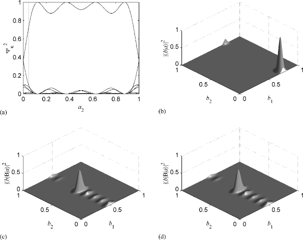
Figure 5: (a) The probabilities $\Psi_{\kappa}^{2}$ when $r=2$. The Husimi functions of (b) the initial state $|a\rangle$ ($a=3/4+i/20$), (c) its mapping $\hat{B}|a\rangle$, and (d) our semi-classical approximation (107), when $r=2$ and $N=8$. The humps have the height $\frac{4}{5}\Psi_{\kappa}^{2}$ with $a_{2}=1/20$ (gray line in (a)).

The probability associated with each hump is given by $\Psi_{\kappa}^{2}$, with $\sum_{\kappa=0}^{2R-1}\Psi_{\kappa}^{2}=1$, and is plotted for $r=2$ in Fig. 5(a). The curve with the largest probabilities is that associated with the ‘correct’ hump prescribed by the classical baker’s map ($\kappa^{\prime}=\lfloor 2a_{1}\rfloor R$). It takes maximum values of unity whenever $a_{2}=(m+1/2)/R$ ($0<m<R-1$), and as the number of momentum bits ($r=\log_{2}R$) becomes large, $\Psi_{\kappa^{\prime}}^{2}\rightarrow 1$ for all $0<a_{2}<1$. Hence, as expected, we are left with a single hump located at the correct position. This agrees with the $0<\theta<1$ case. In figures 5(c) and (d), we have drawn the function $|\langle b|\hat{B}|a\rangle|^{2}$ and its semi-classical approximation (107), respectively, when $a=3/4+i/20$, $r=2$ and $N=8$. For such a large dimension, $D=2^{8}$, our semi-classical approximation becomes almost identical to the exact matrix element. One may also view our semi-classical propagator as an approximation to the Husimi function for the mapped state $\hat{B}|a\rangle$.

IV Conclusion

In this paper, we have derived the semi-classical form of the Schack-Caves quantum baker’s maps, taking into consideration the different possible ways of obtaining the classical limit. We have shown that whenever the number of momentum bits becomes infinite in the limit $\hbar\rightarrow 0$, the quantum propagator in the coherent-state basis takes the Van Vleck form (55). Therefore, we conclude that the classical baker’s transformation is restored for all such cases. In the case where the number of momentum bits is held constant, the classical limit is not that of the baker’s transformation, but a stochastic variant. It may be possible one day to explore this discrepancy experimentally with the help of a quantum computer schack ; brun . As a final note, we remark that although our semi-classical formula (55) espouses a certain familiarity, we should not be presumptuous about its generality. One should, in general, expect extra phases in the exponent (see Baranger et al Baranger ). This has already been found in a spherical geometry for the case of the kicked top Kus1993a .