Understanding Quantum Superarrivals using the Bohmian model

Abstract

We investigate the orgin of “quantum superarrivals” in the reflection and transmission probabilities of a Gaussian wave packet for a rectangular potential barrier while it is perturbed by either reducing or increasing its height. There exists a finite time interval during which the probability of reflection is larger (superarrivals) while the barrier is lowered compared to the unperturbed case. Similarly, during a certain interval of time, the probability of transmission while the barrier is raised exceeds that for free propagation. We compute particle trajectories using the Bohmian model of quantum mechanics in order to understand how this phenomenon of superarrivals occurs.

PACS number(s): 03.65.Bz

A number of interesting investigations have been reported on wave-packet dynamics[1] including, in particular, recent studies on issues such as the observation of revivals of wave packets[2]. Of late, we had pointed out a hitherto unexplored effect[3] considering the time dependent reflection probability of a Gaussian wave packet reflected from a perturbed potential barrier. By reducing the height of the barrier to zero in a short span of time during which there is a significant overlap of it with the wave packet, we observed that the reflection probability is larger compared to the case of reflection from a static barrier for a small but finite interval of time. This phenomenon is what we have called “Quantum Superarrivals”. The speed with which the effect due to reducing the barrier height propagates across the wavefunction was noticed to be depending on the rate at which the barrier height is reduced. We also found the magnitude of superarrivals to be proportional to the rate of reduction of the potential barrier. We argued that superarrivals occur because of the “objective reality” of a wave function acting as a “field” which mediates across it the propagation of a physical disturbance, viz. perturbation of the potential barrier.

The aim of this paper is to further generalize the phenomenon of superarrivals and also to understand how superarrivals occur. We begin by first showing that superarrivals also indeed occur in the transmission probability when the barrier height is raised from zero to some value (this is complementary to the superarrival phenomenon occuring for the reflected wave packet). We then compute particle trajectories using the Bohm model. We derive a quantitative estimate of the magnitude of superarrivals using the Bohmian trajectories. We show that it is possible to obtain a deeper insight into the nature of superarrivals using such computed trajectories of individual particles. We illustrate this by considering the case of a wave packet which is reflected from the perturbed barrier. Similar analysis can be done for the transmitted wave packet.

Let us first briefly recapitulate the essential features of quantum superarrivals. Consider a Gaussian wave packet peaked at $x_{0}$ with half width $\sigma$. It moves to the right and strikes a potential barrier of width $w$ centred at a point $x_{c}$. A detector placed at a point $x^{\prime}$ far left of $x_{0}$ measures the time-dependent reflection probability by counting the reflected particles arriving there up to various instants for both the case of a static barrier, and also when the barrier is perturbed by reducing its height to zero linearly in time. At any instant before the asymptotic value of the reflection probability is attained, the time evolving reflection probability in the region $-\infty<x\leq x\prime$ is given by

$$\left|R(t)\right|^{2}=\int^{x\prime}_{-\infty}\left|\psi\left(x,t\right)\right|^{2}dx$$ (1)

We denote the reflected probability for the static and the perturbed cases as $R_{s}(t)$ and $R_{p}(t)$ respectively. In [3] we computed these probabilities versus time for various values of $\epsilon$ which is the time span over which the barrier height goes to zero (implying different rates of reduction of the potential barrier). We observed that $R_{p}(t)>R_{s}(t)$ during the time interval $t_{d}<t<t_{c}$. If $t_{p}$ is the instant at which the perturbation starts, $t_{c}$ the instant when the static and the perturbed curves cross each other, and $t_{d}$ the time from which the curve corresponding to the perturbed case starts deviating from that in the unperturbed case, we found that $t_{c}>t_{d}>t_{p}$.

Let us now consider the case when initially there is no barrier, and the wave packet is allowed to propagate freely towards the right. A second detector placed far away at $x^{\prime\prime}$ records the time-dependent transmission probability $T_{s}(t)$ (counting the transmitted particles up to various instants of time). If a barrier is raised in the path of the wave packet, a portion of it will be reflected back. We denote by $T_{p}(t)$ the transmitted probability in this case. At any instant before the asymptotic value of the transmission probability ($=1$ since there is no absorption) is attained, the time evolving transmission probability in the region $x^{\prime\prime}\leq x\leq\infty$ is given by

$$\left|T(t)\right|^{2}=\int_{x^{\prime\prime}}^{\infty}\left|\psi\left(x,t\right)\right|^{2}dx$$ (2)

We compute the values of $T_{s}(t)$ and $T_{p}(t)$ using the same method of numerically integrating the time dependent Schrodinger equation as used in [3], which was first developed in [4]. The following values for the parameters are chosen for our computations (in units of $\hbar=1$ and $m=1/2$): $x_{0}=-0.3$, $\sigma=0.05/\sqrt{2}$, $x_{c}=0$, $w=0.016$, $x^{\prime}=-0.5$, $x^{\prime\prime}=0.5$ and $t_{p}=8\times 10^{-4}$. It should be emphasized that the observation of the phenomenon of superarrivals does not hinge upon the choice of these particular values of the parameters. Indeed, the quantitative dependence of superarrivals on the parameter values have been studied in [3] where it was shown that superarrivals in reflection persist for a sufficiently wide range of values of these parameters. We choose one particular set of values for the computations used in this paper since our aim here is primarily to investigate the origin of superarrivals.

The potential barrier is raised from $V=0$ to $V=2E$ (where $E$ is the energy of the incident wave packet) linearly in time $\epsilon$. In Figure 1 we plot the computed values of $T_{s}(t)$ and $T_{p}(t)$ for different values of $\epsilon$. The numbers denoting various instants of time in this as well as the subsequent figures are in units of the time steps used in the numerical algorithm. For example, $t=8\times 10^{-4}$ corresponds to $400$ time steps. It is seen that superarrivals are also exhibited in the transmitted wave packet.

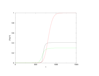
FIG. 1.: The transmission probability $|T(t)|^{2}$ is plotted for various values of $\epsilon$. The top curve reaches value $1$ asymptotically and corresponds to the zero barrier case. The next two curves with ($\epsilon=10$) and ($\epsilon=40$) respectively, represent the transmission probabilities for the rising barriers.

Superarrivals can be quantitatively defined by a parameter $\eta$ given by

$$\eta=\frac{I_{p}-I_{s}}{I_{s}}$$ (3)

where the quantities $I_{p}$ and $I_{s}$ are defined with respect to $\Delta t=t_{c}-t_{d}$ during which superarrivals occur. For the case of superarrivals in the reflected probability,

$$I_{p}=\int_{\Delta t}\left|R_{p}(t)\right|^{2}dt$$ (4)

$$I_{s}=\int_{\Delta t}\left|R_{s}(t)\right|^{2}dt$$ (5)

Replacing the static and perturbed reflected probabilities by $T_{s}(t)$ and $T_{p}(t)$ respectively, one can obtain the corresponding expression of $\eta$ for the case of the transmitted wave packet.

It has been observed[3] that both $\Delta t$ and superarrivals given by $\eta$ depend on the instant $t_{p}$ around which the barrier is perturbed. The magnitude of superarrivals is appreciable only in cases where the wave packet has some significant overlap with the barrier while it is being perturbed. The magnitude of superarrivals falls off with increasing $\epsilon$, for the reflected as well as the transmitted wave packets. Another interesting observation is about information transfer from the perturbing barrier to the detector. We defined signal velocity

$$v_{e}=\frac{D}{t_{d}-(t_{p}-\frac{\epsilon}{2})}$$ (6)

measuring how fast the influence of barrier perturbation travels across the wave packet. We found that $v_{e}$ is again proportional to $\epsilon$ as was the case with $\eta$. These features lead one to argue that the wave packet acts as a carrier (objective field-like behaviour) through which information about the barrier perturbation propagates with a velocity that is proportional to the “disturbance” (measured in terms of the rate of barrier reduction) imparted to the packet by the barrier.

Now, in order to understand how superarrivals originate, we use the concept of particle trajectories in terms of the Bohm model (BM). We recall that BM provides an ontological and a self-consistent interpretation of the formalism of quantum mechanics[6, 7]. Predictions of BM are in agreement with that of standard quantum mechanics. In BM a wave function $\psi$ is taken to be an incomplete specification of the state of an individual particle. An objectively real “position” coordinate (“position” existing irrespective of any external observation) is ascribed to a particle apart from the wave function. Its “position” evolves with time obeying an equation that can be justified in the following way from the Schroedinger equation (considering the one dimensional case)[7]

$$i\hbar{\partial\psi\over\partial t}=H\psi\equiv-{\hbar^{2}\over 2m}{\partial^{2}\psi\over\partial x^{2}}+V(x)\psi$$ (7)

by writing

$$\psi=Re^{iS/\hbar}$$ (8)

and using the continuity equation

$${\partial\over\partial x}(\rho v)+{\partial\rho\over\partial t}=0$$ (9)

with the probability distribution $\rho(x,t)$ being given by

$$\rho=|\psi|^{2}.$$ (10)

It is important to note that $\rho$ in BM is ascribed an ontological significance by regarding it as representing the probability density of “particles” occupying actual positions and the velocity $v$ is interpreted as an ontological (premeasurement) velocity. On the other hand, in the standard interpretation, $\rho$ is interpreted as the probability density of finding particles around specific positions and there is no concept of an ontological velocity. Integrating Eq.(9) by using Eqs.(7), (8) and (10) and requiring that $v$ should vanish when $\rho$ vanishes leads to the Bohmian equation of motion where the particle velocity $v(x,t)$ is given by

$$v\equiv{dx\over dt}={1\over m}{\partial S\over\partial x}$$ (11)

The particle trajectory is thus deterministic and is obtained by integrating the velocity equation for a given initial position.

Another perspective on the notion of particle trajectories in BM is obtained by decomposing the Schrodinger equation in terms of two real equations for the modulus $R$ and the phase $S$ of the wave function $\psi$[6]

$${\partial S\over\partial t}+{(\vec{\nabla}S)^{2}\over 2m}-{\hbar^{2}\over 2m}{\nabla^{2}R\over R}+V=0$$ (12)

$${\partial R^{2}\over\partial t}+\vec{\nabla}.\biggl{(}{R^{2}\vec{\nabla}S\over m}\biggr{)}=0$$ (13)

and by indentifying

$$Q(x,t)=-{\hbar^{2}\over 2m}{\nabla^{2}R\over R}$$ (14)

as the “quantum potential”[6]. The equation of motion of a particle along its trajectory can now be written in a form analogous to Newton’s second law

$${d\over dt}(m\dot{\vec{X}})=-\vec{\nabla}(V+Q)|_{X}$$ (15)

(with $d/dt=\partial/\partial t+\dot{\vec{X}}.\vec{\nabla}$) where the particle is subjected to a quantum force $-\vec{\nabla}Q$ in addition to the classical force $-\vec{\nabla}V$. The effective potential on the particle is $(Q+V)$. We plot the profile of $Q$ versus $x$ at various instants of time near the potential barrier (when its height is reduced) in Figure 2. It is then transparent how the perturbation of the classical potential $V$ affects $Q$ away from the vicinity of the boundary of $V$. This in turn accounts for the sharp turn experienced by those particles which contribute towards superarrivals (as we shall see explicitly later).

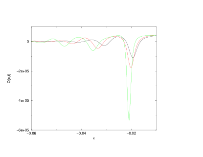
FIG. 2.: Snapshots of the quantum potential $Q(x,t)$ are plotted versus $x$ at various instants of time. The potential barrier is located in the region $-0.008<x<0.008$. Barrier perturbation is from $t=400$ to $t=410$. The full, dashed and dotted curves represent $Q$ at times $t=420$, $425$ and $430$ respectively. The wells in the quantum potential move towards the left with time and reflect incoming particles away from the vicinity of the classical barrier. This explains why certain particles arrive at the detector earlier than they would have done if reflected from a static barrier.

We compute the Bohmian trajectories for a given set of initial positions with a Gaussian distribution corresponding to the initial wave packet. This procedure is carried out for both the cases of lowering and raising the barrier. Since our purpose is to obtain conceptual clarity of the phenomenon of superarrivals, it suffices to illustrate our scheme through the example of superarrivals in the reflection probability when the barrier is reduced. All the qualitative as well as quantitative features of superarrivals are similar in the case where one observes the transmitted probabilty from a rising barrier. Thus, henceforth we consider only the former case in the following discussion.

The following approach is used to study superarrivals in terms of the Bohmian trajectories. First, a particular value of the barrier reduction rate, or $\epsilon$ is chosen. We then choose a range of initial positions for which the trajectory arrival times at the detector lie between $t_{d}$ and $t_{c}$ (i.e., we select only those trajectories which contribute to superarrivals). We consider $N$ such trajectories whose initial positions form a Gaussian distribution. Let us denote one such trajectory by $S_{ip}$ having the initial position $x_{i}$ and the arrival time $t_{ip}$. Taking the static case, the trajectory $S_{i}$ for that initial position $x_{i}$ is computed. Let the corresponding arrival time be $t_{i}$. A supearrival parameter $\beta_{i}$ for the $i$-th Bohmian trajectory is then defined as

$$\beta_{i}={t_{i}-t_{ip}\over t_{i}}$$ (16)

which provides a measure of superarrivals for a particular value of initial position. Next we define an average value

$$\tilde{\beta}={\sum_{i}\beta_{i}\over N}$$ (17)

which provides a quantitative estimate of superarrivals obtained through Bohmian trajectories.

Our results show that the arrival time $t_{ip}$ for the perturbed case is sensitive to the value of initial position $x_{i}$. We have checked that for a particular initial position, $t_{i}$ exceeds $t_{ip}$ for only those trajectories which contribute to superarrivals. This is a distinct feature associated with the superarrivals that can be identified in terms of the Bohmian trajectories. We plot a set of Bohmian trajectories in Figure 3. Note that the trajectories of the particles corresponding to the perturbed case take a sharp turn and arrive at the detector earlier than they would have for a static barrier. Any abrupt perturbation of the potential barrier has thus a global effect on the wave function and affects the values of the quantum potential $Q(x,t)$ at various points. Then, through the Bohmian equation of motion the velocities of the incident particles get correspondingly affected much before reaching the vicinity of the potential barrier. Superarrivals originate from those particles in the perturbed case which reach the detector earlier than those corresponding to the same initial positions in the static case. This accounts for why a detector records more counts in the perturbed case during a particular time interval as compared to that in a static situation. The origin of superarrivals can thus be understood in this way by using the Bohmian trajectories.

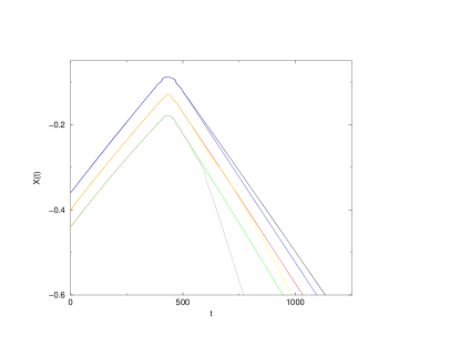
FIG. 3.: Bohmian trajectories for particles originating from the same initial positions get reflected differently from the static and the perturbed barriers. The trajectories undergo sharper turns when the barrier is perturbed and arrive the the detector earlier than they would have done for the static barrier case. The barrier is placed at $x=-0.008$ to $x=0.008$. Perturbation takes place from $t=400$ to $t=410$.

The effect of altering the barrier perturbation time $\epsilon$ on the magnitude of superarrivals $\tilde{\beta}$ can be studied by computing $\tilde{\beta}$ for various values of $\epsilon$. We display the results of this study in Figure 4. Note that the the magnitude of superarrivals decreases monotonically with increasing $\epsilon$, or decreasing rate of perturbation. This effect was also observed in [3] where we obtained a similar behaviour for the superarrival parameter $\eta$. The similarity of these two results obtained through entirely different techniques reinforces our contention about the dynamical nature of superarrivals originating from a “disturbance” provided by the lowering of potential barrier, which propagates across the wave function with a definite speed.

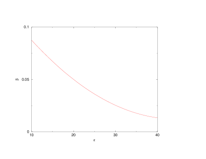
FIG. 4.: The Bohmian superarrival parameter $\tilde{\beta}$ is plotted versus $\epsilon$.

To conclude, in this paper we have explored further the nature and origin of quantum superarrivals manifested in terms of enhanced reflection and transmission probabilities of wave packets from a perturbed potential barrier which is respectively lowered or raised. We have shown how the concept of particle trajectories obtained from the Bohm model enables one to have an insight into the phenomenon of quantum superarrivals. This analysis substantiates our earlier contention[3] that superarrivals arise from a dynamical disturbance provided by the perturbed barrier which propagates across the wave packet (which acts like a “physically real field”) with a definite speed and affects the “particles”. Such time dependent quantum phenomena could be useful in furnishing examples of the conceptual utility of the Bohm model from a perspective different from other examples studied recently [9] for this purpose.

D. Home thanks John Corbett for useful suggestions. Md. Manirul Ali acknowledges the grant of a research fellowship from Council of Scientific and Industrial Research, India.

REFERENCES

- [1] D. M. Greenberger, Physica B 151, 374 (1988); M.V. Berry, J. Phys. A 29, 6617 (1996); M.V. Berry and S. Klein, J. Mod. Opt. 43, 2139 (1996); D.L. Aronstein and C.R. Stroud, Phys. Rev. A 55, 4526 (1997); F. Lillo and R. N. Mantegna, Phys. Rev. Lett. 84, 1061 (2000); G. Kalbermann, J. Phys. A 34, 3841 (2001); G. Kalbermann, quant-ph/0203036.
- [2] See, for instance, A. Venugopalan and G.S. Agarwal, Phys. Rev. A 59, 1413 (1999); F.B.J. Buchkremer, R. Dumke, H. Levsen, G. Birkl and W. Ertmer, Phys. Rev. Lett. 85, 3121 (2000); H. Mack, M. Bienert, F. Haug, F. S. Straub, M. Freyberger and W. P. Schleich, quant-ph/0204040.
- [3] S. Bandyopadhyay, A. S. Majumdar and D. Home, Phys. Rev. A 65, 052718 (2002).
- [4] A. Goldberg, H. M. Schey and J. L. Schwartz, Am. J. Phys. 35, 177 (1967).
- [5] D.Bohm, Phys. Rev. 85, 166 (1952); D.Bohm and B.J.Hiley, “The Undivided Universe”, (Routledge, London, 1993).
- [6] P.R.Holland, “The Quantum Theory of Motion”, (Cambridge University Press, London, 1993).
- [7] E.J. Squires, in “Bohmian Mechanics and Quantum Theory: An Appraisal”, Eds. J.T. Cushing, A. Fine and S. Goldstein (Kluwer, Dordrecht, 1996), pp. 131-140.
- [8] J. G. Muga and C. R. Leavens, Phys. Rep. 338, 353 (2000), and references therein; G. Gruebl and K. Rheinberger, quant-ph/0202084.
- [9] P. Ghose, A. S. Majumdar, S. Guha and J. Sau, Phys. Lett. A 290, 205 (2001); A. S. Majumdar and D. Home, Phys. Lett. A 296, 176 (2002).