Generation of maximum spin entanglement induced by a cavity field
in quantum-dot systems

Abstract

Equivalent-neighbor interactions of the conduction-band electron spins of quantum dots in the model of Imamoḡlu et al. [Phys. Rev. Lett. 83, 4204 (1999)] are analyzed. An analytical solution and its Schmidt decomposition are found and applied to evaluate how much the initially excited dots can be entangled with the remaining dots if all of them are initially disentangled. It is demonstrated that perfect maximally entangled states (MESs) can only be generated in systems of up to six dots with a single dot initially excited. It is also shown that highly entangled states, approximating the MESs with good accuracy, can still be generated in systems of odd numbers of dots with almost half of them excited. A sudden decrease of entanglement is observed on increasing the total number of dots in a system with a fixed number of excitations.

I Introduction

Since the seminal papers of Obermayer, Teich, and Mahler Obe88 , there has been growing interest in the quantum-information properties of quantum dots (QDs) in the quest to implement quantum-dot scalable quantum computers QD-QC ; Loss98 ; QD-spin . Those high expectations are justified to some extent by recent experimental advances in the coherent observation and manipulation of quantum dots Bon98 ; Oos98 , including spectacular demonstrations of the quantum entanglement of excitons in a single dot Chen00 or quantum-dot molecule Bay01 , and observations of Rabi oscillations of excitons in single dots Kam01 . Among various models of quantum computers based on localized electron spins of quantum dots as qubits Loss98 ; QD-spin , the scheme of Imamoḡlu et al. Ima99 is the first, where the interactions between the qubits are mediated by a cavity field. This approach combines the advantages of long-distance optically controlled couplings with long-decoherence times of the spin degrees of freedom. Here, we analyze quantum entanglement in the Imamoḡlu et al. model.

During the last decade, it has been highlighted that quantum entanglement, being at the heart of quantum mechanics, is also a powerful resource for quantum communication and quantum-information processing. Quantum entanglement in interacting systems is a common phenomenon. It is obvious that any interacting many-body system with defined qubits, if set in a properly chosen state, will evolve through states with entangled qubits. Surprisingly, quantitative descriptions of the entanglement dynamics in multiparticle systems are by no means satisfactory yet multipart . Nevertheless, in a special case of bipartite entanglement, a number of measures have been introduced and studied Ben96 ; Ved97 ; Woo98 . For example, entanglement of a bipartite system in a pure state, described by the density matrix $\hat{\rho}_{AB}=(|\psi\rangle\langle\psi|)_{AB}$, can be measured by the von Neumann entropy Ben96 ; Ved97

$$E[\hat{\rho}_{AB}]=-{\rm Tr}\{\hat{\rho}_{A}\log_{2}\hat{\rho}_{A}\}=-{\rm Tr}\{\hat{\rho}_{B}\log_{2}\hat{\rho}_{B}\}$$ (1)

of the reduced density matrix $\hat{\rho}_{A}={\rm Tr}_{B}\{\hat{\rho}_{AB}\}$ or, equivalently, $\hat{\rho}_{B}={\rm Tr}_{A}\{\hat{\rho}_{AB}\}$. The entanglement of formation of a mixed state of a bipartite system is often measured by the so-called concurrence proposed by Hill and WoottersWoo98 . Concurrence has been applied to study entanglement in various models conc including equivalent-neighbor systems Koa00 ; Wang01 . The following two aspects of entanglement are especially important: (i) coherent manipulation of entanglement and (ii) generation of maximum entanglement. The possibility of coherent and selective control of entanglement in a quantum-dot system was analyzed by Imamoḡlu et al. Ima99 . Here, we would like to focus on the latter topic, i.e., the generation of the maximally entangled states (MESs) of quantum dots in the model of Imamoḡlu et al. Ima99 . MESs are necessary for the majority of quantum information-processing applications. Otherwise, for example, direct application of partly entangled states for teleportation will result in unfaithful transmission, while superdense coding with partly entangled states will cause noise in the resulting classical channel.

The paper is organized as follows. In Sec. II, we describe an equivalent-neighbor quantum-dot model and give its analytical solution. In Sec. III, we analyze the possibilities of generation of the MESs or their good approximations for different initial conditions of the number of excitations and the total number of dots in the system.

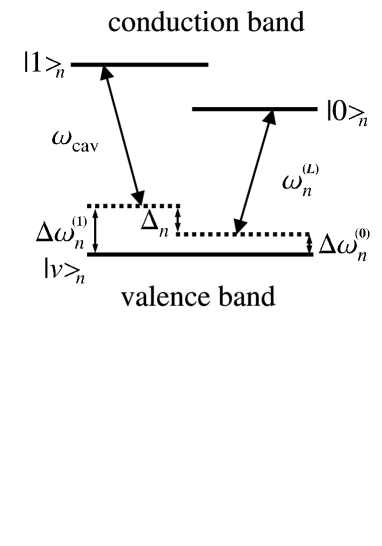
Figure 1: Three-level atom in $V$ configuration as a model of a semiconductor dot with the conduction-band spin states $|1\rangle_{n}$ (spin up) of energy ${\cal E}_{n}^{(1)}$ and $|0\rangle_{n}$ (spin down) of energy ${\cal E}_{n}^{(0)}$ , and the effective valence-band state $|v\rangle_{n}$ of energy ${\cal E}_{n}^{(v)}$ in the $n$th dot. Key: $\omega_{{\rm cav}}$, frequency of the common cavity mode; $\omega_{n}^{(L)}$, frequency of the classical laser field addressed at the $n$th dot; $\hbar\Delta\omega_{n}^{(1)}={\cal E}_{n}^{(1)}-{\cal E}_{n}^{(v)}-\hbar\omega_{{\rm cav}}$, $\hbar\Delta\omega_{n}^{(0)}={\cal E}_{n}^{(0)}-{\cal E}_{n}^{(v)}-\hbar\omega_{n}^{(L)}$, and $\Delta_{n}=\Delta\omega_{n}^{(1)}-\Delta\omega_{n}^{(0)}$ are detunings.

II Quantum-dot model and its solution

We will apply the model of Imamoḡlu et al. Ima99 to describe strong equivalent-neighbor couplings of quantum-dot spins through a single-mode microcavity field. The dots are placed inside a microdisk, put into a microcavity tuned to frequency $\omega_{{\rm cav}}$, and illuminated selectively by laser fields of frequencies $\omega_{n}^{(L)}$. Each of $N$ dots with a single electron in the conduction band is modeled by a three-level atom as shown in Fig. 1. The total Hamiltonian for $N$ three-level quantum dots interacting with $N+1$ quantized fields reads

$$\hat{H} = \hat{H}_{QD}+\hat{H}_{F}+\hat{H}_{\rm int},$$ (2)

$$\hat{H}_{QD} = \sum_{n}({\cal E}_{n}^{(0)}\hat{\sigma}_{n}^{00}+{\cal E}_{n}^{(1)}\hat{\sigma}_{n}^{11}+{\cal E}_{n}^{(v)}\hat{\sigma}_{n}^{vv}),$$

$$\hat{H}_{F} = \hbar\omega_{{\rm cav}}\hat{a}_{{\rm cav}}^{{\dagger}}\hat{a}_{{\rm cav}}+\sum_{n}\hbar\omega_{n}^{(L)}(\hat{a}_{n}^{(L)})^{{\dagger}}\hat{a}_{n}^{(L)},$$

$$\hat{H}_{\rm int} = \sum_{n}\hbar g_{n}^{v0}[\hat{a}_{n}^{(L)}\hat{\sigma}_{n}^{0v}+(\hat{a}_{n}^{(L)})^{{\dagger}}\hat{\sigma}_{n}^{v0}]$$

$$+\sum_{n}\hbar g_{n}^{v1}(\hat{a}_{{\rm cav}}\hat{\sigma}_{n}^{1v}+\hat{a}_{{\rm cav}}^{{\dagger}}\hat{\sigma}_{n}^{v1}),$$

where $\hat{H}_{QD}$ and $\hat{H}_{F}$ are the free Hamiltonians of the quantum dots and the fields, respectively; $\hat{H}_{\rm int}$ is the interaction Hamiltonian; $\hat{a}_{\rm cav}$ and $\hat{a}^{{\dagger}}_{\rm cav}$ are the annihilation and creation operators of the cavity mode, respectively; $\hat{a}^{(L)}_{n}$ and $(\hat{a}^{(L)}_{n})^{{\dagger}}$ are the corresponding operators for the laser modes; $\hat{\sigma}_{n}^{xy}$ is the $n$th dot operator given by $\hat{\sigma}_{n}^{xy}=|x\rangle_{nn}\langle y|$; ${\cal E}_{n}^{(x)}$ is the energy of level $|x\rangle_{n}$ ($x=0,1,v$); the $n$th dot levels $|0\rangle_{n}$ and $|v\rangle_{n}$ are coupled by dipole interactions with a strength of $g_{n}^{v0}$; analogously, $g_{n}^{v1}$ is the coupling strength between levels $|1\rangle_{n}$ and $|v\rangle_{n}$. There is no direct coupling between levels $|0\rangle_{n}$ and $|1\rangle_{m}$ in either the same ($n=m$) or different dots ($n\neq m$). The Hamiltonian (2) simply generalizes, to $N$ dots and $N+1$ fields, models of a three-level atom (dot) interacting with two modes of radiation fields widely discussed in the literature (see, e.g., 3plus2 ). By applying an adiabatic elimination method, Imamoḡlu et al. derived the effective interaction Hamiltonian describing the evolution of the conduction-band spins of $N$ quantum dots coupled by a microcavity field in the form Ima99

$$\hat{H}_{{\rm eff}} = \!\frac{\hbar}{2}\sum_{n\neq m}\kappa_{nm}(t)[{\hat{\sigma}}_{n}^{+}{\hat{\sigma}}_{m}^{-}e^{i(\Delta_{n}-\Delta_{m})t}$$ (3)

$$~{}~{}~{}~{}~{}~{}~{}~{}~{}~{}~{}~{}~{}~{}~{}~{}+{\hat{\sigma}}_{n}^{-}{\hat{\sigma}}_{m}^{+}e^{-i(\Delta_{n}-\Delta_{m})t}]$$

in terms of the Pauli spin creation ${\hat{\sigma}}_{n}^{+}$ and annihilation ${\hat{\sigma}}_{n}^{-}$ operators acting on the conduction-band spin states of the $n$th dot. The effective two-dot coupling strength between the spins of the $n$th and $m$th dots is given by $\kappa_{nm}(t)=g_{n}(t)g_{m}(t)/\Delta_{n}$, where the effective single-dot coupling of the $n$th spin to the cavity field is $g_{n}(t)=g_{n}^{v0}g_{n}^{v1}|E^{(L)}_{n}(t)|/\Delta\omega_{n}$ with $\Delta\omega_{n}$ being the harmonic mean of $\Delta\omega_{n}^{(1)}$ and $\Delta\omega_{n}^{(0)}$. For simplicity, the laser fields are assumed to be strong and treated classically as described by the complex amplitudes $E^{(L)}_{n}(t)$. The Hamiltonian (3) was derived by applying adiabatic eliminations of the valence-band states $|v\rangle_{n}$ and cavity mode $\hat{a}_{{\rm cav}},$ which are valid under the assumptions of negligible coupling strength, cavity decay rate, and thermal fluctuations in comparison to $\hbar\Delta_{n}$ and $\hbar\Delta\omega_{n}^{(x)}$ ($x=0,1$) and the energy difference ${\cal E}_{n}^{(1)}-{\cal E}_{n}^{(0)}$ (see Fig. 1). Moreover, the valence-band levels $|v\rangle_{n}$ were assumed to be far off resonance. Although the Hamiltonian (3) describes apparently direct spin-spin interactions, the real physical picture is different: Quantum-dot spins are coupled only indirectly via the cavity and laser fields.

Imamoḡlu et al. Ima99 applied their model for quantum computing purposes by implementing the conditional phase-flip and controlled-NOT (CNOT) operations between two arbitrary dots addressed selectively by laser fields to satisfy the condition $\Delta_{n}=\Delta_{m}$. Here, we are interested in a realization of an equivalent-neighbor model scalable for a large number of dots (even for more than 100 Ima99 ). This goal can readily be achieved by assuming that all dots are identical and illuminated by a single-mode stationary laser field of frequency $\omega_{n}^{(L)}\equiv\omega^{(L)}$, which implies $\kappa_{nm}(t)=\kappa=\,$const. In fact, the condition of equivalent-neighbor interactions can also be assured for nonidentical dots by adjusting the laser-field frequencies $\omega_{n}^{(L)}$ to get the same detuning $\Delta_{n}=\,$const, and by choosing the proper laser intensities $|E^{(L)}_{n}|^{2}$ to obtain the effective coupling constants of $g_{n}(t)=\,$const or, equivalently, $\kappa_{nm}(t)=\,$const for every pair of dots. Thus, Eq. (3) can be reduced to the effective equivalent-neighbor $N$-dot Hamiltonian as

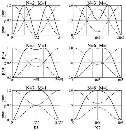
Figure 2: Evolution of the quantum entanglement of $E^{N1}(t)$ (solid) and the Schmidt coefficients of $P_{0}^{N1}(t)$ (dashed) and $P_{1}^{N1}(t)$ (dot-dashed curves) for systems of $N=2,\cdots,8$ quantum dots with only one ($M=1$) of them initially excited. Figure illustrates that the exact maximally entangled states can be generated in systems of $N$ up to 6 dots only.

$$\hat{H}_{\rm eff}=\frac{\hbar\kappa}{2}\sum_{n\neq m}\left({\hat{\sigma}}_{n}^{+}{\hat{\sigma}}_{m}^{-}+{\hat{\sigma}}_{n}^{-}{\hat{\sigma}}_{m}^{+}\right)$$ (4)

where $\kappa$ is the coupling constant. The system described by Eq. (4) is sometimes referred to as the spin-$1/2$ van der Waals model Dek79 , the infinitely coordinated system Bot82 , the Lipkin or Lipkin-Meshkov-Glick model Lip65 , or just the equivalent-neighbor model Liu90 . Let us assume that the initial state describing a system of $M$ ($M=0,\cdots,N$) dots initially excited (i.e., with conduction-band spins up) and $N-M$ dots in the ground state (conduction-band spins down) is given as

$$|\psi(0)\rangle = \{|1\rangle^{\otimes M}\}_{A}\{|0\rangle^{\otimes(N-M)}\}_{B}$$ (5)

$$\equiv |\underbrace{11\cdots 1}_{M}\rangle_{A}|\underbrace{00\cdots 0}_{N-M}\rangle_{B}.$$

Then, we find the solution of the Schrödinger equation of motion for the model (4) in the form

$$|\psi(t)\rangle = \sum_{m=0}^{M^{\prime}}C_{m}^{NM}(t){\{|1\rangle^{\otimes(M-m)}|0\rangle^{\otimes m}\}}_{A}$$ (6)

$$~{}~{}~{}~{}~{}~{}~{}~{}~{}~{}~{}~{}\otimes{\{|1\rangle^{\otimes m}|0\rangle^{\otimes(N-M-m)}\}}_{B},$$

where $M^{\prime}=\min(M,N-M)$. The states in curly brackets $\{|1\rangle^{\otimes(n-m)}|0\rangle^{\otimes m}\}$ denote the sum of all $n$-dot states with $(n-m)$ excitations. For example, ${\{|1\rangle^{\otimes 2}|0\rangle^{\otimes 2}\}}$ stands for $|0011\rangle+|0101\rangle+|0110\rangle+|1001\rangle+|1010\rangle+|1100\rangle$. The number of states in the superposition $\{|1\rangle^{\otimes(n-m)}|0\rangle^{\otimes m}\}$ (or equivalently $\{|1\rangle^{\otimes m}|0\rangle^{\otimes(n-m)}\}$) is equal to the binomial coefficient $\textstyle{n\choose m}$. Thus, for given $N$ and $M$, the solution (6) contains $\textstyle{N\choose M}$ terms. The energy of the QD system described by Eq. (4) is conserved; thus all the superposition states in Eq. (6) have the same number $M$ of excitations. We find the time-dependent superposition coefficients in Eq. (6) as

$$C_{m}^{NM}(t) = \sum_{n=0}^{M^{\prime}}b_{nm}^{NM}\exp\big{\{}i[n(N+1-n)$$ (7)

$$~{}~{}~{}~{}~{}~{}~{}~{}~{}~{}~{}~{}~{}~{}~{}~{}-M(N-M)]\kappa t\big{\}}$$

in terms of

$$b_{nm}^{NM} = \sum_{k=0}^{m}(-1)^{k}{m\choose k}{N-2k\choose M-k}^{-1}$$ (8)

$$~{}~{}~{}\times\left[{N+1-2k\choose n-k}-2{N-2k\choose n-k-1}\right],$$

where $\textstyle{x\choose y}$ are binomial coefficients. Our solution can be represented in a biorthogonal form via the Schmidt decomposition

$$|\psi(t)\rangle=\sum_{m=0}^{M^{\prime}}\sqrt{P_{m}^{NM}(t)}|\phi_{m}(t)\rangle_{A}\otimes|\varphi_{m}(t)\rangle_{B},$$ (9)

where $|\phi_{m}(t)\rangle_{A}$ and $|\varphi_{m}(t)\rangle_{B}$ are the orthonormal basis states of subsystems $A$ and $B$, respectively. We find that the real and positive Schmidt coefficients can be related to the squared module of superposition coefficients (7) as follows:

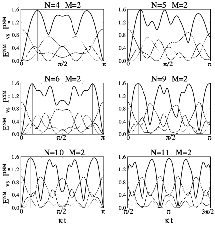
Figure 3: Evolution of the entanglement of $E^{N2}(t)$ (solid) and all Schmidt coefficients $P_{0}^{N2}(t)$ (dashed), $P_{1}^{N2}(t)$ (dot-dashed), and $P_{2}^{N2}(t)$ (dotted curves), in systems with two ($M=2$) dots initially excited.

$$P_{m}^{NM}(t)={M\choose m}{N-M\choose m}|C_{m}^{NM}(t)|^{2},$$ (10)

while the phases of $C_{m}^{NM}(t)$ are absorbed into the definition of the basis states $|\phi_{m}(t)\rangle_{A}$ and $|\varphi_{m}(t)\rangle_{B}$. The Schmidt coefficients are normalized to unity. The evolutions of all $P_{m}^{NM}$ for systems with single and two excitations are given in Figs. 2 and 3, respectively. We observe that the evolution of Schmidt coefficients is periodic with the period of $\kappa T=2\pi/N$ for systems with a single ($M=1$ or, equivalently, $M=N-1$) excitation (Fig. 2), and $\pi$ periodical ($2\pi$ periodical) for systems of even (odd) numbers of dots with higher numbers of excitations (see Fig. 3). For brevity, only half of the period is depicted in the right-hand panels of Fig. 3.

III Entanglement in quantum-dot systems

We address the following questions: How much can the initially excited dots (say, subsystem $A$) be entangled with the remaining dots (subsystem $B$) in the equivalent-neighbor system of initially all disentangled dots if the evolution is governed by Hamiltonian (4)? And whether the maximally entangled states can be generated exactly or, at least, approximately in systems of an arbitrary number $N$ of dots while $M$ of them are excited.

With the help of an explicit form of the Schmidt decomposition, it is convenient to calculate the entanglement (1) via the Shannon entropy

$$E^{NM}(t) \equiv E[|\psi(t)\rangle\langle\psi(t)|]$$ (11)

$$= -\sum_{m=0}^{M^{\prime}}P_{m}^{NM}(t)\log_{2}P_{m}^{NM}(t)$$

of the Schmidt coefficients given for our system by (10). By applying Eq. (11), we can determine the maximum entanglement given by $E^{NM}_{\max}(t)\equiv\max_{t}E^{NM}(t)$, which can periodically be generated during the evolution of $N$-dot system with $M$ excitations. The coefficients (10), as well as (7), possess the symmetry of $P_{m}^{NM}(t)=P_{m}^{N,N-M}(t)$, which implies equal evolutions of entanglement

$$E^{NM}(t)=E^{N,N-M}(t)$$ (12)

in the $N$-dot systems with $M$ and $N-M$ excitations. Figure 4 shows this symmetry in a special case for maximum entanglement of $\max_{t}E^{NM}(t)=\max_{t}E^{N,N-M}(t)$.

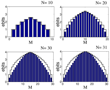
Figure 4: Maximum entanglement $E_{\max}^{NM}=\max_{t}E^{NM}(t)$ (solid bars), measured in ebits, as a function of the excitation number $M$ generated in systems of $N=10,20,30$ and 31 dots. The empty staircase corresponds to entanglement of $E_{\rm MES}^{NM}$ for the MESs. The figure illustrates that the highest entanglement, closest to $E_{\rm MES}^{NM}$, can be generated in systems with $M=[N/2]$ excitations. On decreasing $M$ or ($N-M$), the entanglement decreases. The discrepancy between $E_{\max}^{NM}$ and $E_{\rm MES}^{NM}$ becomes more pronounced with increasing $N$ especially for $0<M\ll[N/2]$.

To solve the second problem proposed at the beginning of this section, we have to determine the quantum correlations of the maximally entangled state of two subsystems having $d$ equally weighted terms in its Schmidt decomposition. According to the theorem of Bennett et al. Ben96 , the MES has $\log_{2}d$ ebits of entanglement, where $d$ is the Hilbert space dimension of the smaller subsystem. Thus, in our case, the MES of the subsystem $A$ consisting of $M$ dots and the subsystem $B$ of $N-M$ dots has

$$E_{{\rm MES}}^{NM}=\log_{2}[\min(M,N-M)+1]$$ (13)

ebits of entanglement. In particular, the MES in the $N$-dot system with a single initial excitation has only 1 ebit independent of $N$. The empty staircase in Fig. 4 and solid lines in Fig. 5 correspond to $E_{{\rm MES}}^{NM}$. To show a deviation of a given state from the MES, it is convenient to use the relative (or scaled) entanglement defined to be

$$e^{NM}_{\max}\equiv\frac{E^{NM}_{\max}}{E^{NM}_{{\rm MES}}}=\max_{t}\frac{E^{NM}(t)}{E^{NM}_{\rm MES}}.$$ (14)

In the simplest nontrivial case, for $M=1$, the Schmidt coefficients reduce to

$$P_{1}^{N1}(t)=4{{\frac{(N-1)}{N^{2}}}}\sin^{2}\left(\frac{N}{2}\kappa t\right)$$ (15)

and $P_{0}^{N1}(t)=1-P_{1}^{N1}(t)$, which enable a direct calculation of the entanglement $E^{N1}(t)$ with the help of Eq. (11). The evolutions of entanglement and the Schmidt coefficients of $P_{m}^{N1}(t)$ for $m$=0,1, are depicted in Fig. 2. The quantum-dot systems evolve into the MESs at evolution times that are the roots of the equation

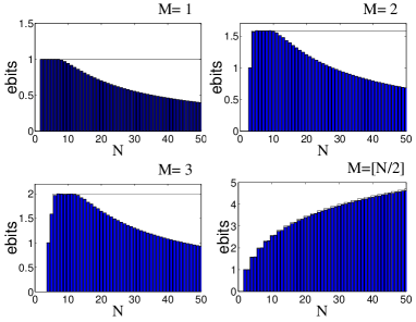
Figure 5: Maximum entanglement $E_{\max}^{NM}$ as a function of the total number $N$ of dots generated in systems with $M$=1,2,3, and $[N/2]$ excitations. The solid lines and empty staircase correspond to $E_{\rm MES}^{NM}$. On the scale of the figure, an apparent plateau occurs for $N$ smaller than some critical value $N_{M}$. For $N$ higher than $N_{M}$ and fixed $M$, a monotonic decrease of the maximum entanglement is clearly visible. One concludes that arbitrary high entanglement can be achieved by increasing $N$ and keeping half $M=[N/2]$ of the system excited.

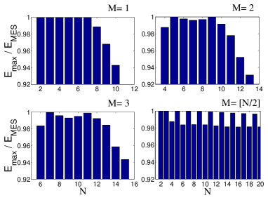
Figure 6: The same as in Fig. 5 but for the relative maximum entanglement $e_{\max}^{NM}=E_{\max}^{NM}/E_{\rm MES}^{NM}$. The figure shows that the apparent plateau for finite $M$ actually occurs for $M=1$ only. The first and second highest maxima of entanglement correspond to $N$ equal to $2M+1$ and $2M+5$, respectively.

$$0=\dot{E}^{NM}(t) = 2\kappa{{\frac{N-1}{N}}}\sin(N\kappa t)$$ (16)

$$\times \!\!\log_{2}\left[{{\frac{N^{2}}{4(N-1)}}}\csc^{2}\left({{\frac{N}{2}}}\kappa t\right)-1\right].$$

Thus, we get

$$\kappa t^{\prime}={{\frac{2}{N}}}{\rm arccsc}\left({{\frac{2}{N}}}\sqrt{2(N-1)}\right)$$ (17)

and $\kappa t^{\prime\prime}=\pi/N$. We find that the maximum entanglement, equal to ${E}^{N1}(t^{\prime})=1$ ebit, can be achieved at evolution times $t^{\prime}$ for $N\leq 6$ only. For $N>6$, a real solution for $t^{\prime}$ does not exist. Another explanation of this result, as illustrated in Fig. 2, can be given as follows: The maximum entanglement corresponds to the Schmidt coefficients mutually equal or, in general, the least different. But the MES corresponds solely to the former case. As seen in Fig. 2, the condition $P_{0}^{N1}(t^{\prime})=P_{1}^{N1}(t^{\prime})$ is strictly satisfied for $N\leq 6$. The entanglement for $N>6$ reaches its maximum at evolution times $t^{\prime\prime}$. This maximum value is given by

$${E}^{N1}(t^{\prime\prime}) = {{\frac{2}{N^{2}}}}\big{\{}N^{2}\log_{2}N-(N-2)^{2}\log_{2}(N-2)$$ (18)

$$~{}~{}~{}~{}~{}-2(N-1)\log_{2}[4(N-1)]\big{\}},$$

which is less than unity and monotonically decreases with increasing $N$ as clearly illustrated in Figs. 5 and 6 for $M$=1. Thus, the perfect MESs cannot be generated in systems of $N>6$ dots. Nevertheless, a good approximation of the MESs can also be obtained for $N=7$. On the scale of Fig. 2, $\max_{t}E^{7,1}(t)=E^{7,1}(\pi/7)=0.9997$ is close to unity since $P_{0}^{N1}(\pi/7)$ and $P_{1}^{N1}(\pi/7)$ are almost the same. It is worth noting that a critical value of $N=6$ was also found, although in the different context of the pairwise entanglement measured by the concurrence Woo98 , for an equivalent-neighbor model of entangled webs in Ref. Koa00 . In comparison, a critical value of $N=6$ for the concurrence in the equivalent-neighbor isotropic or anisotropic Heisenberg models was not observed (see, e.g., Wang01 ). Similarly, generation of the MESs in an equivalent-neighbor quantum-dot model of Reina et al. was discussed only in two special cases of the Bell ($N$=2) and Greenberger-Horne-Zeilinger (GHZ) ($N$=3) entangled states Rei00 . Thus, no critical behavior of entanglement as a function of $N$ was reported there.

The case for $M=1$ is the only one where the general formula (10) for the Schmidt coefficients simplifies to a compact form for arbitrary evolution times. Thus, for clarity, we present mainly numerical results for $M\geq 2$. For example, Fig. 3 illustrates that the exact MESs cannot be generated in systems with $M=2$ excitations at any evolution time. This conclusion can be drawn from the observation that $P_{m}^{N2}(t)$ for $m$=0,1,2 do not cross simultaneously at any times in the period. Nevertheless, the MESs can be approximated with good precision. The highest possible entanglement, corresponding to the least mutually different $P_{m}^{N2}$, is observed for $N=5$ and 9, where the relative entanglement deviates from unity at the order of $10^{-5}$ and $10^{-4}$, respectively (see Fig. 6 for $M$=2). The states generated in $N$-dot systems with three excitations can be entangled up to $e^{7,3}_{\max}=0.9996$ (first) and $e^{11,3}_{\max}=0.9990$ (second maximum) for the relative entanglement (see Fig. 6 for $M$=3). It is interesting to compare the relative entanglement of $e^{NM}_{\max}$, depicted in Fig. 6, with the “absolute” entanglement of $E^{NM}_{\max}$ presented in Fig. 5. By analyzing the numerical data given, in part, in Fig. 6, we find the following rule: The maximally or almost maximally entangled states can be generated in systems of $N=2M+1$ dots with $M$ excitations. Slightly worse entanglement can be achieved in systems of $N=2M+5$ dots with $M$ excitations. Thus, systems composed of odd rather than even numbers of dots enable generation of the entangled states better approximating the MESs for $M>1$. This is clearly illustrated in Fig. 6 for $M=[N/2]$, i.e., the integer part of $N/2$. We observe that the system of odd and large numbers ($N>2M+5$ for $M>1$) of dots is the most entangled at evolution times $\kappa t=(1+2k)\pi$ for $k=0,1,...$ (see, e.g., Fig. 3 for $N$=11). In this special case, the Schmidt coefficients can be written compactly via

$$\left|C_{m}^{NM}\left(\frac{\pi}{\kappa}\right)\right|=2^{m}m!(N-2M)\frac{(N-2m-2)!!}{N!!}.$$ (19)

For $\kappa t=k\pi$ and even $N$, in contrast to odd $N$, the entanglement vanishes. The maximum entanglement of $E^{NM}_{\max}$ for $N>N_{M}\equiv 2M+5-\delta_{1M}$ can be well fitted by the inverse of linear functions as shown in Fig. 7.

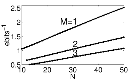
Figure 7: The inverse of the maximum entanglement, $(E_{\max}^{NM})^{-1}$ (dots) measured in ebits^-1, and its approximation (solid lines) as a function of $N>2M+5$ generated in systems with $M=1,2,3$ excitations.

IV Conclusion

We studied the evolution of the conduction-band spins of quantum dots in the model of Imamoḡlu et al. Ima99 . We found the analytical solution and its Schmidt decomposition for the equivalent-neighbor model and applied them in our study of bipartite entanglement in quantum-dot systems with arbitrary numbers of dots and their excitations. We have raised and solved the problem to what extent the initially excited dots can be entangled with the remaining dots if all of them are initially disentangled in the equivalent-neighbor energy-conserving model. We have shown that the perfect maximally entangled states can only be generated in systems of $N=2,\cdots,6$ dots with a single dot initially excited. Nevertheless, highly entangled states, being excellent approximations of the MESs, can periodically be generated in systems of odd numbers $N$ of dots with the number $M$ of excitations equal to $M=(N-1)/2$ (leading to the best approximation) and $M=(N-5)/2$ (giving a slightly worse approximation). If we increase $N$ beyond $N_{M}=2M+5-\delta_{1M}$, the entanglement decreases monotonically as described by the inverse of linear functions.

published in the Physical Review A 65 (2002) 062321 and selected to Virtual J. Nanoscale Sci. Tech. (http://www.vjnano.org/nano/) 6 (2002) Issue 1; Virtual J. Quantum Information (http://www.vjquantuminfo.org) 2 (2002) Issue 7.

References

- (1) K. Obermayer, W. G. Teich, and G. Mahler, Phys. Rev. B 37, 8096 (1988); 37, 8111 (1988).
- (2) A. Barenco et al., Phys. Rev. Lett. 74, 4083 (1995); H. Matsueda and S. Takeno, IEICE Trans. Fundamentals E79-A, 1707 (1996); H. Matsueda, Superlattices Microstr. 24, 423 (1998); G. D. Sanders et al., Phys. Rev. A 60, 4146 (1999); E. Biolatti et al., Phys. Rev. Lett. 85, 5647 (2000).
- (3) D. Loss and D. P. DiVincenzo, Phys. Rev. A 57, 120 (1998); G. Burkard et al., Phys. Rev. B 59, 2070 (1999).
- (4) S. N. Molotkov, JETP Lett. 64, 237 (1996); S. Bandyopadhyay, Phys. Rev. B 61, 13 813 (2000); T. Ohshima, Phys. Rev. A 62, 062316 (2000); J. Levy, . 64, 052306 (2001).
- (5) N. H. Bonadeo et al., Science 282, 1473 (1998).
- (6) T. H. Oosterkamp et al., Nature (London) 395, 873 (1998).
- (7) G. Chen et al., Science 289, 1966 (2000).
- (8) M. Bayer et al., Science 291, 451 (2001).
- (9) T. H. Stievater et al., Phys. Rev. Lett. 87, 133603 (2001); H. Kamada et al., . 87, 246401 (2001).
- (10) A. Imamoḡlu et al., Phys. Rev. Lett. 83, 4204 (1999); Fortschr. Phys. 48, 987 (2000).
- (11) M. Murao et al., Phys. Rev. A 57, R4075 (1998); A. Thapliyal, 59, 3336 (1999); C. H. Bennett et al., . 63, 012307 (2000); W. Dür et al., Phys. Rev. Lett. 83, 3562 (1999); N. Linden et al., . 83, 243 (1999); H. A. Carteret et al., Found. Phys. 29, 527 (1999).
- (12) C. H. Bennett et al., Phys. Rev. A 53, 2046 (1996).
- (13) V. Vedral et al., Phys. Rev. Lett. 78, 2275 (1997); V. Vedral and M. B. Plenio, Phys. Rev. A 57, 1619 (1998).
- (14) S. Hill and W. K. Wootters, Phys. Rev. Lett. 78, 5022 (1997); W. K. Wootters, . 80, 2245 (1998).
- (15) W. K. Wootters, e-print quant-ph/0001114; K. M. O’Connor and W. K. Wootters, Phys. Rev. A 63, 052302 (2001); D. Gunlycke et al., 64, 042302 (2001); M. C. Arnesen, S. Bose, and V. Vedral, Phys. Rev. Lett. 87, 017901 (2001).
- (16) M. Koashi, V. Bužek, and N. Imoto, Phys. Rev. A 62, 050302 (2000).
- (17) X. Wang and K. Mølmer, Eur. Phys. J. D 18, 385 (2002).
- (18) J. H. Reina et al., Phys. Rev. A 62, 012305 (2000).
- (19) C. C. Gerry and J. H. Eberly, Phys. Rev. A 42, 6805 (1990); M. Alexanian and M. Bose, . 52, 2218 (1995); Y. Wu, . 54, 1586 (1996).
- (20) R. Dekeyser and M. H. Lee, Phys. Rev. B 19, 265 (1979); 43, 8123 (1991); 43, 8131 (1991).
- (21) R. Botet et al., Phys. Rev. Lett. 49, 478 (1982).
- (22) H. J. Lipkin, N. Meshkov, and A. J. Glick, Nucl. Phys. 62, 188 (1965).
- (23) J.-M. Liu and G. Müller, Phys. Rev. A 42, 5854 (1990); Phys. Rev. B 44, 12 020 (1991).