Nonclassical statistics of intracavity coupled $\chi^{(2)}$ waveguides: the quantum optical dimer

Abstract

A model is proposed where two $\chi^{(2)}$ nonlinear waveguides are contained in a cavity suited for second-harmonic generation. The evanescent wave coupling between the waveguides is considered as weak, and the interplay between this coupling and the nonlinear interaction within the waveguides gives rise to quantum violations of the classical limit. These violations are particularly strong when two instabilities are competing, where twin-beam behavior is found as almost complete noise suppression in the difference of the fundamental intensities. Moreover, close to bistable transitions perfect twin-beam correlations are seen in the sum of the fundamental intensities, and also the self-pulsing instability as well as the transition from symmetric to asymmetric states display nonclassical twin-beam correlations of both fundamental and second-harmonic intensities. The results are based on the full quantum Langevin equations derived from the Hamiltonian and including cavity damping effects. The intensity correlations of the output fields are calculated semi-analytically using a linearized version of the Langevin equations derived through the positive-$P$ representation. Confirmation of the analytical results are obtained by numerical simulations of the nonlinear Langevin equations derived using the truncated Wigner representation.

PACS: 42.50.Dv, 42.50.Lc, 42.65.Sf, 42.65.Wi

I Introduction

The $\chi^{(2)}$ nonlinear materials have been the subject of various investigations in recent years. Using a cavity setup the weak nonlinearities can be resonantly amplified, and complex spatiotemporal behavior has been predicted from a classical point of view [1]. Moreover, due to the quantum fluctuations of light many interesting non-classical effects have been reported, such as squeezed light [2] and sub-Poissonian light [3], both theoretically [4, 5] and experimentally [6, 7]. The interplay between the classical spatial instabilities and the quantum fluctuations in the system has been investigated intensively lately [1], a study devoted to characterizing the mode interaction on the quantum level.

We consider the case of second-harmonic generation (SHG), where the photons of the pump field (fundamental photons) are up-converted in pairs to second-harmonic photons of the double frequency. The model we propose in this paper consists of two quadratically nonlinear waveguides placed in a cavity that resonates both the fundamental and second-harmonic, and we take linear coupling between the waveguides into account. In a sense this is the simplest mode coupling model obtainable. The question is how the coupling between the waveguides affects the cavity dynamics, and in particular we shall focus on the nonclassical behavior of the system.

The name proposed for this model, the quantum optical dimer, originates from the numerous investigations made about discrete site coupling in various systems, such as condensed matter physics and biology, see Ref.[8] for a general treatment of discrete systems. Thus, the name dimer implies that coupling between two discrete sites are being taken into account. For a single waveguide (or site) we shall use the name monomer, a case corresponding here to a bulk nonlinear medium and neglecting diffraction.

It has been shown that in the SHG quantum optical monomer excellent squeezing of the output fields is possible close to a self-pulsing instability [5], and nonclassical effects in SHG have been verified experimentally [7], and even shown to persist above the threshold of the instability [9]. Also in the presence of diffraction strong correlations exist between different spatial modes in the presence of a spatial instability [10], including strong correlations between the fundamental field and the generated second-harmonic field as well as spatial multimode nonclassical light.

As we shall show the quantum optical dimer also displays strong nonclassical correlations in the intensity correlations, and that the linear coupling across the waveguides plays a decisive role. The model has three types of transitions, bistability, self-pulsing and a symmetric to asymmetric transition. It is remarkable that particularly strong nonclassical correlations are observed when two of these instabilities compete. Specifically, when taken close to a self-pulsing or bistable regime the symmetric to asymmetric transition has nearly perfect twin-beam behavior, so the difference of the fundamental intensities displays almost no fluctuations. The twin-beam correlations were first shown in the optical parametric oscillator (OPO) [11, 12], where the signal and idler photons of the twin-fields are generated simultaneously from the pump field, and the intensity difference shows correlations below the classical limit. However, the twin-beam effect observed in the dimer originates from photons created in different waveguides with only the coupling to link them. Thus, the photons are strictly speaking not twins, but merely “brothers”. The twin-beam effect is also observed near bistable turning points where complete noise suppression is observed in the sum of the fundamental intensities, the strongest violations occurring in the limit where the fundamental input coupling loss rate is much larger than the second-harmonic one. That bistability gives rise to highly nonclassical effects turns out to also hold for the SHG monomer, and has to our knowledge not been observed before; usually the self-pulsing transition has been used to observe violations of the classical limit, which we also observe in the dimer. The bistable transition has previously been observed to produce nonclassical states in other systems, such as dispersive and absorptive optical bistability [5, 13] and Raman lasers [14].

A closely related optical model is spatially coupled lasers [15], where a single laser medium is pumped by two beams spatially separated. Waveguiding is achieved by thermal lensing, in which the temperature dependent refractive index of the laser medium creates a guiding effect, and the coupling strength is controlled by the distance between the pump profiles. The quantum noise induced correlations in these systems have not yet been reported to beat the standard quantum limit when Kerr type nonlinearities are considered [16, 17], except when the coupling arises solely due to initially correlated noise terms of the pumps [18].

The cavityless setup of coupled $\chi^{(2)}$ waveguides has previously been investigated, both from a classical and a quantum mechanical point of view. In the classical model of waveguide arrays, the focus of attention has been on soliton behavior originating from the coupling [19], whereas the cavityless dimer was shown to produce chaotic states away from the integrable limit (where second-harmonic coupling is neglected) [20]. The quantum behavior of the cavityless dimer has been investigated by the group of Perina et al. (for a review see Ref. [21]) giving the name “nonlinear coupler” to the model. They have investigated both co- and counter-propagating input fields in parametric oscillation and, e.g., the transfer of quantum states from one waveguide to the other.

The model presented here is also closely related to the dynamics of coupled atomic and molecular Bose-Einstein condensates (BECs) [22, 23], where the photoassociation of an atomic condensate may produce a molecular condensate with an atom-molecule interaction that is reminiscent of the interaction between the fundamental and second-harmonic photons in SHG [24]. The opposite process where the photo dissociation of a molecular BEC creates an atomic BEC has been shown to produce squeezed states [25], a model which has the quantum optical equivalent in the OPO. If an analogy should be drawn between the quantum optical dimer presented here and BEC it would consist of placing two such coupled molecular-atomic BECs in separate quantum wells. Thus, evanescent tunneling of the wave functions between the wells would introduce the dimer coupling, similar to what is done in Ref. [26] for a normal BEC.

We should finally stress that the cavity setup discussed in the present work gives rise to two major differences to the work in cavityless waveguides as well as for the BEC. First of all the cavity introduces losses in the model through the input mirror, and secondly external pump fields appear in the equations acting as forcing terms.

The paper is structured as follows. In Sec. II the model is introduced, and the stochastic Langevin equations are derived from the full boson operator Hamiltonian. Also, we discuss the allowed values of the coupling constants. In Sec. III the linear stability of the Langevin equations are investigated, and the bifurcation scenario of the model is discussed. In Sec. IV we discuss the framework for the two-time photon number correlations of the output fields, and the semi-analytical spectral variances are derived in the linearized limit. Section V is devoted to the results of the analytical calculations as well as the numerical simulations. A summary is made in Sec. VI where we also discuss the results obtained. Appendix A shows details about the derivation of the quasi-probability distribution equations used to connect the master equation for the quantum Hamiltonian with the classical looking stochastic Langevin equations. The numerical methods are discussed in App. B.

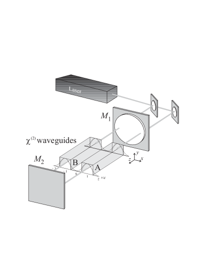
FIG. 1.: The setup. Two nonlinear waveguides A and B inside a cavity pumped by a classical field.

II The model

We consider the setup shown in Fig. 1. Two $\chi^{(2)}$ nonlinear waveguides are contained in a cavity with a high reflection input mirror $M_{1}$ and a fully reflecting mirror $M_{2}$ at the other end. The cavity is pumped at the frequency $\omega_{1}$ and through the nonlinear interaction in the waveguides photons of the frequency $\omega_{2}=2\omega_{1}$ are generated; this is the process of second-harmonic generation. The cavity supports a discrete number of longitudinal modes, and we will consider the case where only two of these modes are relevant, namely the mode $\omega_{1,{\mathrm{c}av}}$ closest to the fundamental-harmonic (FH) frequency and $\omega_{2,{\mathrm{c}av}}$ closest to the second-harmonic (SH) frequency. Using the mean field approximation the $z$-direction, in which the pump beam propagates, is averaged out. This approach is justified as long as the losses and detunings are small, and we furthermore assume perfect phase matching. The waveguiding implies that diffraction in the transverse plane may be neglected. Let $\hat{A}_{1}(t)$ and $\hat{B}_{1}(t)$ ($\hat{A}_{2}(t)$ and $\hat{B}_{2}(t)$) denote the FH (SH) intracavity boson operators of waveguide A and B, respectively. They are normalized so they obey the following equal time commutation relations

$$[\hat{O}_{i}(t),\hat{O}_{j}^{\dagger}(t)]=\delta_{ij},\quad i,j=1,2,\quad\hat{O}=\hat{A},\hat{B},$$ (1)

while $[\hat{A}_{j}(t),B^{\dagger}_{j}(t)]=0$. The system is modelled through the Hamiltonian

$$\hat{H}=\hat{H}^{\mathrm{s}ys}_{A}+\hat{H}^{\mathrm{s}ys}_{B}+\hat{H}_{AB},$$ (2)

where the system Hamiltonians in the frame rotating with the pump frequency are given by

$$\hat{H}^{\mathrm{s}ys}_{O} = -\hbar\delta_{1}\hat{O}_{1}^{\dagger}\hat{O}_{1}-\hbar\delta_{2}\hat{O}_{2}^{\dagger}\hat{O}_{2}+\frac{i\hbar\kappa}{2}({\hat{O}^{\dagger 2}_{1}}\hat{O}_{2}-\hat{O}_{1}^{2}\hat{O}_{2}^{\dagger})$$ (4)

$$+i\hbar({\mathcal{E}}_{{\mathrm{p}},O}\hat{O}_{1}^{\dagger}-{\mathcal{E}}_{{\mathrm{p}},O}^{*}\hat{O}_{1}),\quad O=A,B.$$

The detunings from the cavity resonances are given by $\delta_{j}=\omega_{j}-\omega_{j,\mathrm{c}av}$, $\kappa$ is proportional to the $\chi^{(2)}$ nonlinearity and ${\mathcal{E}}_{{\mathrm{p}},O}$ are the external pump fields at the FH frequency of the individual waveguides [27], here treated as classical fields. The coupling between the waveguides is modelled as overlapping tails of evanescent waves so it may be assumed weak, implying we can describe it as a linear process

$$\hat{H}_{AB}=\hbar J_{1}(\hat{A}_{1}\hat{B}_{1}^{\dagger}+\hat{B}_{1}\hat{A}_{1}^{\dagger})+\hbar J_{2}(\hat{A}_{2}\hat{B}_{2}^{\dagger}+\hat{B}_{2}\hat{A}_{2}^{\dagger}).$$ (5)

$J_{1}$ and $J_{2}$ are the cross-waveguide coupling parameters of the FH and SH, respectively. The time evolution of the reduced system density matrix operator $\hat{\rho}$ in the Schrödinger picture is then given by the master equation [28, 29]

$$\frac{\partial\hat{\rho}}{\partial t}=-\frac{i}{\hbar}[\hat{H},\hat{\rho}]+(\hat{L}_{1,A}+\hat{L}_{2,A}+\hat{L}_{1,B}+\hat{L}_{2,B})\hat{\rho}.$$ (6)

The continuum of modes outside the cavity is modelled as a heat bath in thermal equilibrium, and the coupling to these modes has been included through the Liouvillian terms

$$\hat{L}_{j,O}\hat{\rho} = \gamma_{j}\left([\hat{O}_{j},\hat{\rho}\hat{O}_{j}^{\dagger}]+[\hat{O}_{j}\hat{\rho},\hat{O}_{j}^{\dagger}]\right)$$ (8)

$$+\gamma_{j}\bar{n}^{\mathrm{t}h}_{j}\left([\hat{O}_{j}\hat{\rho},\hat{O}_{j}^{\dagger}]+[\hat{O}_{j}^{\dagger},\hat{\rho}\hat{O}_{j}]\right).$$

These terms describe the losses of the fields through photons escaping the cavity, and simultaneously they model fluctuations entering the cavity through the input mirror, a consequence of the dissipation-fluctuation theorem [30]. The loss rates of the input coupling mirror are given by $\gamma_{j}$, whereas the terms $\bar{n}^{\mathrm{t}h}_{j}=(e^{\hbar\omega_{j}/k_{B}T}-1)^{-1}$ are the mean number of thermal quanta in the external bath modes at $\omega_{j}$. We shall here neglect thermal fluctuations by setting the bath temperature $T=0$ yielding $\bar{n}^{\mathrm{t}h}_{j}=0$. First of all this is a good approximation for optical systems since here $\hbar\omega\gg k_{B}T$, and secondly we may hereby focus on behavior solely due to the inherent quantum fluctuations of light.

The master equation (6) is difficult to solve as it is, therefore we apply the now standard technique of expanding the density matrix in a basis of coherent states weighted by a quasi-probability distribution (QPD). The details of this quantum-to-classical description are given in App. A, and the result is a partial differential equation of the QPD. This QPD equation depends on the choice of ordering of the corresponding quantum mechanical averages. Equation (A17) is the QPD equation using the positive-$P$ distribution giving normally ordered averages, which we will use for the linearized analysis. For the numerical implementation the Wigner distribution is used to obtain Eq. (A19), in which symmetric averages are calculated.

If the QPD equations (A17) and (A19) are on the Fokker-Planck form (A28), an equivalent set of stochastic Langevin equations (A29) can be found to by using Ito rules of stochastic integration [31]. For the Wigner QPD equation (A19) this is not the case because of the third order terms, however these terms, which have been shown to model quantum jump processes [32], are generally neglected and the resulting Fokker-Planck equation turns out to be a good approximation to the original problem. Using this approximation the normalized Langevin equations for the Wigner QPD equation are

$$\dot{A}_{1} = (-1+i\Delta_{1})A_{1}+A_{1}^{*}A_{2}-iJ_{1}B_{1}+\sqrt{2}A_{{\mathrm{i}n},1}(t)$$ (10)

$$\dot{A}_{2} = (-\gamma+i\Delta_{2})A_{2}-\frac{1}{2}A_{1}^{2}-iJ_{2}B_{2}+\sqrt{2\gamma}A_{{\mathrm{i}n},2}(t)$$ (11)

$$\dot{B}_{1} = (-1+i\Delta_{1})B_{1}+B_{1}^{*}B_{2}-iJ_{1}A_{1}+\sqrt{2}B_{{\mathrm{i}n},1}(t)$$ (12)

$$\dot{B}_{2} = (-\gamma+i\Delta_{2})B_{2}-\frac{1}{2}B_{1}^{2}-iJ_{2}A_{2}+\sqrt{2\gamma}B_{{\mathrm{i}n},2}(t),$$ (13)

where the dot denotes derivation with respect to time. The fields $\{A_{j},A_{j}^{*}\}$ and $\{B_{j},B_{j}^{*}\}$ are normalized equivalent $c$-numbers to the operators $\{\hat{A}_{j},\hat{A}_{j}^{\dagger}\}$ and $\{\hat{B}_{j},\hat{B}_{j}^{\dagger}\}$. The input fields are describing the pump field entering the cavity through the input mirror as well as the noise coupled in here according to the Liouvillian terms (8)

$$F_{{\mathrm{i}n},1}(t)=\frac{E}{\sqrt{2}}+\xi_{F_{1}}(t),\quad F_{{\mathrm{i}n},2}(t)=\xi_{F_{2}}(t)$$ (15)

$$\langle\xi_{F_{i}}^{*}(t)\xi_{F_{j}}(t^{\prime})\rangle=\delta_{ij}\frac{\delta(t-t^{\prime})}{2n_{s}},$$ (16)

with $F=A,B$. All other correlations are zero. The positive-$P$ QPD equation (A17) is on Fokker-Planck form so no approximations are needed. The equivalent set of Langevin equations is given by (II) with $A_{j}^{*}\rightarrow A_{j}^{\dagger}$ and $B_{j}^{*}\rightarrow B_{j}^{\dagger}$, as well as the equations for the fields

$$\dot{A}_{1}^{\dagger} = (-1-i\Delta_{1})A_{1}^{\dagger}+A_{1}A_{2}^{\dagger}$$ (19)

$$+iJ_{1}B_{1}^{\dagger}+\sqrt{2}A^{\dagger}_{{\mathrm{i}n},1}(t)$$

$$\dot{A}_{2}^{\dagger} = (-\gamma-i\Delta_{2})A_{2}^{\dagger}-\frac{1}{2}(A_{1}^{\dagger})^{2}$$ (21)

$$+iJ_{2}B_{2}^{\dagger}+\sqrt{2\gamma}A^{\dagger}_{{\mathrm{i}n},2}(t)$$

$$\dot{B}_{1}^{\dagger} = (-1-i\Delta_{1})B_{1}^{\dagger}+B_{1}B_{2}^{\dagger}$$ (23)

$$+iJ_{1}A_{1}^{\dagger}+\sqrt{2}B^{\dagger}_{{\mathrm{i}n},1}(t)$$

$$\dot{B}^{\dagger}_{2} = (-\gamma-i\Delta_{2})B_{2}^{\dagger}-\frac{1}{2}(B_{1}^{\dagger})^{2}$$ (25)

$$+iJ_{2}A_{2}^{\dagger}+\sqrt{2\gamma}B^{\dagger}_{{\mathrm{i}n},2}(t).$$

The fields $\{A_{j},A_{j}^{\dagger}\}$ and $\{B_{j},B_{j}^{\dagger}\}$ are normalized equivalent $c$-numbers to the operators $\{\hat{A}_{j},\hat{A}_{j}^{\dagger}\}$ and $\{\hat{B}_{j},\hat{B}_{j}^{\dagger}\}$. The input fields for the positive-$P$ Langevin equations are

$$F_{{\mathrm{i}n},1}(t)=\frac{E}{\sqrt{2}}+\xi_{F_{1}}(t),\quad F^{\dagger}_{{\mathrm{i}n},1}(t)=\frac{E}{\sqrt{2}}+\xi^{\dagger}_{F_{1}}(t)$$ (27)

$$F_{{\mathrm{i}n},2}(t)=0,\quad F^{\dagger}_{{\mathrm{i}n},2}(t)=0$$ (28)

$$\langle\xi_{F_{1}}(t)\xi_{F_{1}}(t^{\prime})\rangle=\frac{F_{2}\delta(t-t^{\prime})}{2n_{s}}$$ (29)

$$\langle\xi^{\dagger}_{F_{1}}(t)\xi^{\dagger}_{F_{1}}(t^{\prime})\rangle=\frac{F_{2}^{\dagger}\delta(t-t^{\prime})}{2n_{s}},$$ (30)

with $F=A,B$, and again all other correlations are zero. The doubling of phase space associated with the positive-$P$ representation (see App. A for details) implies that $\xi_{j}^{\dagger}$ is uncorrelated to $\xi_{j}$, and also that $A_{j}$ and $A_{j}^{\dagger}$ are independent complex numbers and only on average is $A_{j}^{\dagger}=A_{j}^{*}$.

The Langevin equations have been normalized by introducing the dimensionless variables

$$\tilde{t}=\gamma_{1}t,\quad\gamma=\frac{\gamma_{2}}{\gamma_{1}},\quad\Delta_{j}=\frac{\delta_{j}}{\gamma_{1}}$$ (32)

$$A_{j}=\frac{\kappa}{\gamma_{1}}\alpha_{j},\quad B_{j}=\frac{\kappa}{\gamma_{1}}\beta_{j}$$ (33)

$$A_{{\mathrm{i}n},j}(\tilde{t})=\frac{\kappa}{\gamma_{1}^{3/2}}\alpha_{{\mathrm{i}n},j}(t),\quad B_{{\mathrm{i}n},j}(\tilde{t})=\frac{\kappa}{\gamma_{1}^{3/2}}\beta_{{\mathrm{i}n},j}(t)$$ (34)

$$\tilde{\xi}_{j}(\tilde{t})=\frac{\kappa}{\gamma_{1}^{3/2}}\xi_{j}(t),\quad E=\frac{\kappa}{\gamma_{1}^{2}}{\mathcal{E}}_{\mathrm{p}},\quad\tilde{J}_{j}=\frac{J_{j}}{\gamma_{1}},$$ (35)

and the tildes have been dropped. The fields $\alpha_{j}$ and $\beta_{j}$ are the unscaled $c$-numbers, cf. App. A. We have furthermore introduced the dimensionless quantity

$$n_{s}=\kappa^{2}/\gamma_{1}^{2}.$$ (36)

This parameter sets the level of the quantum noise, cf. Eqs. (II) and (II), and in the OPO it represents the saturation photon number to trigger the parametric oscillation.

For simplicity we have assumed real and equal pump rates in both waveguides ${\mathcal{E}}_{{\mathrm{p}},A}={\mathcal{E}}_{{\mathrm{p}},B}\equiv{\mathcal{E}}_{{\mathrm{p}}}$. The consequence is that the same input mirrors as well as intracavity paths are used for both waveguides, implying identical detunings [33] as well as losses for the FH fields and the SH fields, respectively.

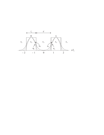
FIG. 2.: Parallel planar waveguide setup shown in the $x$-direction. The width of the waveguides is $l_{\mathrm{w}}$ and the distance between them is $d$. The transverse distributions of the lowest order modes for a realistic setup are shown calculated using a step profile of the refractive index.

The coupling strengths between the waveguides are controlled by $J_{1}$ and $J_{2}$, and it is relevant to consider what values these may take. Fig. 2 shows an instructive example, where we consider symmetric step-index parallel planar waveguides with a core (cladding) refractive index $n_{\mathrm{c}o}$ ($n_{\mathrm{c}l}$). The weakly guiding limit is assumed where $n_{\mathrm{c}o}\simeq n_{\mathrm{c}l}$. Taking the FH field of waveguide A as example, the coupling from waveguide B can be found by considering waveguide A in isolation and taking the presence of waveguide B as a weak perturbation. This approach assumes that the transverse profile $u(x)$ and propagation constant $\beta$ of the modes in the waveguides are left unchanged, and only the amplitude is modified by the perturbation. The coupling constants of the propagation equations of the waveguides are then found as [34]

$$J_{A_{1}B_{1}}=\frac{n_{\mathrm{c}o}^{2}-n_{\mathrm{c}l}^{2}}{2}\frac{k_{1}^{2}}{\beta_{A_{1}}}\int_{-d/2-l_{\mathrm{w}}}^{-d/2}dx\;u_{A_{1}}(x)u_{B_{1}}(x),$$ (37)

where $k_{1}=2\pi/\lambda_{1}$ is the vacuum wavenumber of the FH, and the mode profiles are assumed normalized so $\int_{-\infty}^{\infty}dxu^{2}(x)=1$. Thus, Eq. (37) has the dimension m^-1. Fig. 2 shows the lowest order modes of the isolated waveguides as calculated for a realistic setup. If only coupling between modes of same order is considered we have $J_{A_{1}B_{1}}=J_{B_{1}A_{1}}\equiv J_{1}^{\mathrm{p}rop}$. Applying the mean field approach [35] the coupling parameters of Eqs. (II) is then given by $J_{j}=J_{j}^{\mathrm{p}rop}L_{\mathrm{c}av}/\tau_{1}$, where $L_{\mathrm{c}av}$ is the length of the cavity, and $\tau$ is the cavity round trip time. From Eq. (35) the normalized coupling parameter is found through $\gamma_{1}=T_{1}/(2\tau)$ where $T_{1}$ is the FH intensity transmission efficiency of the input mirror, so we obtain [36]

$$\tilde{J}_{j}=J_{j}^{\mathrm{p}rop}\frac{2L_{\mathrm{c}av}}{T_{1}}.$$ (38)

As a result of these considerations we see that the SH coupling parameter generally will be lower than the FH one. This is clear from the calculated modes in Fig. 2, where the SH modes (dashed) decay faster than the FH modes (solid). However, it is impossible to generally say how much weaker and when the distance between the waveguides is decreased the coupling parameters become closer to each other. Finally, the actual values of $\tilde{J}_{j}$ are highly sensitive to the specific setup. Not only in terms of waveguide parameters (e.g., distance between guides, the modes in the guides), but also on independent parameters (cavity length, input transmission efficiency). Using parameters from realistic setups (similar to the cavity setup discussed in Ref. [37]) we easily obtained normalized coupling parameters of $O(10^{2})$, while still preserving the assumptions of weak coupling as well as the mean-field limit. Finally, when coupling between the lowest order modes is considered we have $J_{j}>0$.

III Linear stability

In this section the Langevin equations derived previously are linearized and the linear stability is investigated to obtain a bifurcation scenario in the classical limit where noise is absent ($n_{s}\rightarrow\infty$). In this limit the Langevin equations from the different representations give the same result, a natural consequence from the fact that in the classical limit the operators commute. Additionally, in Sec. IV we are going to use the linearized equations with noise to derive analytical results for the noise induced correlations. For this purpose it is more convenient to use normally ordered intracavity averages, as will be explained later, and this section will therefore only concern the positive-$P$ Langevin equations. The results of this section reveal both symmetric and asymmetric modes in the two waveguides, as well as bistable behavior and Hopf unstable solutions.

The linearization is particularly simple in the symmetric case. Here the steady states in the waveguides are identical, so the FH steady states in waveguide A and B are equal and equivalently for the SH steady states. The symmetric steady states of the waveguides can be found from the monomer equations, i.e. using the results of Ref. [38] and apply the substitution $\Delta_{j}\rightarrow\Delta_{j}-J_{j}\equiv d_{j}$. In the symmetric case the steady states are denoted ${\mathcal{A}}_{j}={\mathcal{B}}_{j}\equiv\sqrt{\bar{I}_{j}}e^{i\phi_{j}}$ giving

$$E^{2} = \bar{I}_{1}^{2}\frac{\bar{I}_{1}/4+(\gamma-d_{1}d_{2})}{d_{2}^{2}+\gamma^{2}}+\bar{I}_{1}(d_{1}^{2}+1)$$ (40)

$$\bar{I}_{2} = \bar{I}_{1}^{2}[4(d_{2}^{2}+\gamma^{2})]^{-1}$$ (41)

$$\phi_{1} = -{\mathrm{A}rg}\left(1-id_{1}+\bar{I}_{1}/[2(\gamma-id_{2})]\right)$$ (42)

$$\phi_{2} = -{\mathrm{A}rg}(-\gamma+id_{2})+2\phi_{1}.$$ (43)

We may linearize the positive-$P$ Langevin equations (II), (II) and (II) around the symmetric steady states $A_{j}=\Delta A_{j}+{\mathcal{A}}_{j}$ and $B_{j}=\Delta B_{j}+{\mathcal{A}}_{j}$ [39] to get the matrix equation

$$\Delta\dot{\mathbf{w}}={\mathbf{A}}\Delta{\mathbf{w}}+\frac{{\mathbf{B}}}{\sqrt{n_{s}}}{\mathbf{n}}(t),$$ (44)

where $\Delta{\mathbf{w}}$ is a vector of fluctuations

$$\Delta{\mathbf{w}}=\left[\Delta{A_{1}},\Delta A_{1}^{\dagger},\Delta{A_{2}},\Delta A_{2}^{\dagger},\Delta{B_{1}},\Delta B_{1}^{\dagger},\Delta{B_{2}},\Delta B_{2}^{\dagger}\right]^{T},$$ (45)

and ${\mathbf{n}}(t)$ is a vector of Gaussian white noise terms correlated as

$$\langle n_{j}(t)n_{k}(t^{\prime})\rangle=\delta(t-t^{\prime}).$$ (46)

The matrix ${\mathbf{A}}$ is block ordered into four $4\times 4$ matrices

$${\mathbf{A}}=\begin{bmatrix}{\mathbf{A}}_{m}&{\mathbf{A}}_{x}\\ {\mathbf{A}}_{x}&{\mathbf{A}}_{m}\\ \end{bmatrix},$$ (47)

with the diagonal cross-coupling matrix

$${\mathbf{A}}_{x} =\mathrm{Diag}\left[\begin{array}[]{cccc}-iJ_{1}&iJ_{1}&-iJ_{2}&iJ_{2}\\ \end{array}\right],$$ (49)

and the monomer matrix is

$${\mathbf{A}}_{m} =\begin{bmatrix}-1+id_{1}&{\mathcal{A}}_{2}&{\mathcal{A}}_{1}^{*}&0\\ {\mathcal{A}}_{2}^{*}&-1-id_{1}&0&{\mathcal{A}}_{1}\\ -{\mathcal{A}}_{1}&0&-\gamma+id_{2}&0\\ 0&-{\mathcal{A}}_{1}^{*}&0&-\gamma-id_{2}\\ \end{bmatrix}.$$ (50)

The diffusion matrix is also diagonal

$${\mathbf{D}} =\mathrm{Diag}\begin{bmatrix}{\mathcal{A}}_{2}&{\mathcal{A}}_{2}^{*}&0&0&{\mathcal{A}}_{2}&{\mathcal{A}}_{2}^{*}&0&0\\ \end{bmatrix},$$ (51)

and ${\mathbf{D}}={\mathbf{B}}^{T}{\mathbf{B}}$.

The classical stability of the system is found by solving the eigenvalue problem ${\mathbf{A}}{\mathbf{v}}=\lambda{\mathbf{v}}$, which is done in Mathematica. The analysis is characterized by two cases, either when one physical solution exists to the closed problem (40)-(41), or when the system is bistable and three physical solutions exist (in this case each solution must be analyzed individually). The stability of the steady states may now either change with the critical eigenvalue $\lambda_{j,c}$ having ${\mathrm{I}m}(\lambda_{j,c})=0$ at the critical pump value $E_{\mathrm{s}ym}$, which means that the symmetric state of the system is no longer stable. When this happens a new state with ${\mathcal{A}}_{j}\neq{\mathcal{B}}_{j}$ is stable instead, and the actual values of these new steady states are not easily calculated. We will not address the stability of the system beyond the asymmetric transition any further in this paper, however the transition to the asymmetric state will be used to look for nonclassical correlations. The other possibility is that the system changes stability with ${\mathrm{I}m}(\lambda_{j,c})\neq 0$ at the critical pump value $E_{\mathrm{S}P}$, which corresponds to a Hopf instability leading to self-pulsing temporal oscillations.

The system is well characterized by the relative loss rate $\gamma$, which in the SHG monomer was shown to determine the degree of squeezing as well as which field the best squeezing was observed [5]. Following the simple layout of the cavity shown in Fig. 1 implies that $\Delta_{1}=\Delta_{2}\equiv\Delta$ [33]. The bifurcation scenario in the $\{J_{1},\Delta\}$ space for $J_{2}=1.0$ is shown in Fig. 3, which displays a rich variety of behavior. For $\Delta<1$ bistable behavior is observed, and the upper branch may be both Hopf unstable as well as asymmetrically unstable as indicated. For $\Delta>1$ a large Hopf region is seen, while for $J_{1}$ large, asymmetric states are observed.

Setting $\gamma=1$ a similar scenario as for $\gamma=0.1$ is observed: On resonance self-pulsing symmetric states dominates, while bistable solutions may be seen for $\Delta<-1$ and asymmetric states appear when $\Delta>0$. For $\gamma=10$ the self-pulsing instability dominates and asymmetric solutions only appear when detuning is introduced and simultaneous large values of $J_{1}$ and $J_{2}$ are chosen. Bistable solutions are not seen here except for very large coupling strengths, a consequence of the criteria for bistability (Eq. (6) in Ref. [38])

$$\frac{|d_{2}|(|d_{1}|-\sqrt{3})}{\sqrt{3}|d_{1}|+1}>\gamma,\quad d_{1}d_{2}>0.$$ (52)

All these results indicate that the most diverse bifurcation scenario is when $\gamma\leq 1$.

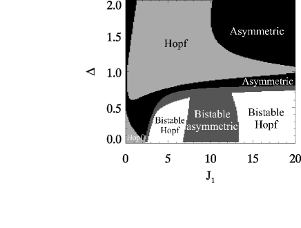
FIG. 3.: Bifurcation diagram showing the stability for $\Delta_{1}=\Delta_{2}=\Delta$, $\gamma=0.1$ and $J_{2}=1.0$. In the bistable area the stability of the upper branch is indicated.

IV Photon number spectra

The linearized Langevin equation for the positive-$P$ representation can be used to analytically calculate the spectrum of fluctuations in the stationary state, provided that the fluctuations are small. These intracavity fluctuation correlations can be directly related to the output correlations by using the input-output theory of Gardiner and Collett [40]. We will only present results in the case where the symmetric steady states are stable.

The input fields $\hat{O}_{{\mathrm{i}n},j}(t)$ coupled into the cavity through the input mirror are posing an instantaneous boundary condition for the output fields

$$\hat{O}_{{\mathrm{o}ut},j}(t)=\sqrt{2\gamma_{j}}\hat{O}_{j}(t)-\hat{O}_{{\mathrm{i}n},j}(t),\quad\hat{O}=\hat{A},\hat{B}.$$ (53)

It should be stressed that in this equation $\gamma_{j}$ is only the loss rate of the input mirror, and does not include additional absorption losses of the cavity that might otherwise have been included in the Langevin equations. Also note that the input operator is in the FH taken as a both the classical pump as well as the fluctuations around this classical level originating from the heat bath interaction [so really an operator equivalent of the Langevin input fields from Eqs. (II) and (II)]. The fields outside the cavity obey the standard free field commutator relations

$$[\hat{O}_{{\mathrm{o}ut},j}(t),\hat{O}_{{\mathrm{o}ut},k}^{\dagger}(t^{\prime})]=\delta_{jk}\delta(t-t^{\prime}),$$ (54)

and

$$[\hat{O}_{{\mathrm{i}n},j}(t),\hat{O}_{{\mathrm{i}n},k}^{\dagger}(t^{\prime})]=\delta_{jk}\delta(t-t^{\prime}),$$ (55)

while all other commutators are zero. We want to express correlations of the out fields entirely on correlations of the intra cavity fields, hence we want to get rid of terms involving $\hat{O}_{{\mathrm{i}n},j}(t)$. Using arguments of causality it may be shown that this can only be done if time and normally ordered correlations are considered [40], as e.g.

$$\langle\hat{A}_{{\mathrm{o}ut},j}^{\dagger}(t),\hat{A}_{{\mathrm{o}ut},j}(t^{\prime})\rangle=2\gamma_{j} \langle\hat{A}_{j}^{\dagger}(t),\hat{A}_{j}(t^{\prime})\rangle$$ (57)

$$\langle\hat{A}_{{\mathrm{o}ut},j}(t),\hat{A}_{{\mathrm{o}ut},j}(t^{\prime})\rangle=2\gamma_{j} \langle\hat{A}_{j}(\mathrm{max}[t,t^{\prime}]),$$ (59)

$$\;\;\hat{A}_{j}(\mathrm{min}[t,t^{\prime}])\rangle,$$

which precisely implies time and normal order of the correlations. Since this is exactly what the $P$-representation computes the intracavity operator averages on the right hand side of Eq. (55) may be directly replaced by $c$-number averages from the $P$-representation.

The intensities of the output beams may be found from the photon number operator $\hat{N}^{O}_{{\mathrm{o}ut},j}=\hat{O}_{{\mathrm{o}ut},j}^{\dagger}\hat{O}_{{\mathrm{o}ut},j}$. In a photon counting experiment two-time correlations of the intensities may be calculated as

$$C_{A_{j}B_{k}}^{(\pm)}(\tau) \equiv \langle\hat{N}^{A}_{{\mathrm{o}ut},j}(t)\pm\hat{N}^{B}_{{\mathrm{o}ut},k}(t),\hat{N}^{A}_{{\mathrm{o}ut},j}(t+\tau)\pm\hat{N}^{B}_{{\mathrm{o}ut},k}(t+\tau)\rangle$$ (60)

$$= (\langle\hat{N}^{A}_{{\mathrm{o}ut},j}\rangle+\langle\hat{N}^{B}_{{\mathrm{o}ut},k}\rangle)\delta(\tau)+\langle:\hat{N}^{A}_{{\mathrm{o}ut},j}(t)\pm\hat{N}^{B}_{{\mathrm{o}ut},k}(t),\hat{N}^{A}_{{\mathrm{o}ut},j}(t+\tau)\pm\hat{N}^{B}_{{\mathrm{o}ut},k}(t+\tau):\rangle$$ (61)

$$= 2(\gamma_{j}\langle\hat{N}^{A}_{j}\rangle+\gamma_{k}\langle\hat{N}^{B}_{k}\rangle)\delta(\tau)+4\langle:\delta\hat{N}_{A_{j}B_{k}}^{(\pm)}(t),\delta\hat{N}_{A_{j}B_{k}}^{(\pm)}(t+\tau):\rangle,$$ (62)

where the notation $\langle:\;:\rangle$ indicates a normally ordered average. In the second line we have used the commutator relations (54) to rewrite to normal order, while the last line follows from Eq. (55). We have also introduced

$$\delta\hat{N}_{A_{j}B_{k}}^{(\pm)}(t)=\gamma_{j}\hat{N}^{A}_{j}(t)\pm\gamma_{k}\hat{N}^{B}_{k}(t),\quad\hat{N}^{O}_{j}=\hat{O}_{j}^{\dagger}\hat{O}_{j},$$ (63)

and calculated the variance as $\langle S,T\rangle\equiv\langle ST\rangle-\langle S\rangle\langle T\rangle$.

It is more convenient to investigate these two-time correlations in the Fourier frequency domain using the Wiener-Khintchine theorem [30]

$$V_{A_{j}B_{k}}^{(\pm)} (\omega)=\int_{-\infty}^{\infty}d\tau e^{i\omega\tau}C_{A_{j}B_{k}}^{(\pm)}(\tau)$$ (68)

$$=2(\gamma_{j}\langle\hat{N}^{A}_{j}\rangle+\gamma_{k}\langle\hat{N}^{B}_{k}\rangle)$$

$$+4\int_{-\infty}^{\infty}d\tau e^{i\omega\tau}\langle:\delta\hat{N}_{A_{j}B_{k}}^{(\pm)}(t),\delta\hat{N}_{A_{j}B_{k}}^{(\pm)}(t+\tau):\rangle$$

$$\equiv 2(\gamma_{j}\langle\hat{N}^{A}_{j}\rangle+\gamma_{k}\langle\hat{N}^{B}_{k}\rangle)\bar{V}_{A_{j}B_{k}}^{(\pm)}(\omega).$$

Here we have introduced the spectrum normalized to shot-noise $\bar{V}_{A_{j}B_{k}}^{(\pm)}(\omega)$, and the shot-noise level given by

$$C_{SN}=2(\gamma_{j}\langle\hat{N}^{A}_{j}\rangle+\gamma_{k}\langle\hat{N}^{B}_{k}\rangle),$$ (69)

is with this normalization unity. The shot-noise level is the limit between classical and quantum behavior, hence if $\hat{A}_{j}$ and $\hat{B}_{k}$ are coherent states the variance will be $\bar{V}_{A_{j}B_{k}}^{(\pm)}(\omega)=1$. A complete violation of the shot-noise level $\bar{V}_{A_{j}B_{k}}^{(\pm)}(\omega)=0$ implies that no fluctuations are associated with the measurement of the intensities $\hat{N}^{A}_{{\mathrm{o}ut},j}\pm\hat{N}^{B}_{{\mathrm{o}ut},k}$. The correlations between the fields of the same waveguide are

$$C_{A_{j}}(\tau) \equiv \langle\hat{N}^{A}_{{\mathrm{o}ut},j}(t),\hat{N}^{A}_{{\mathrm{o}ut},j}(t+\tau)\rangle$$ (70)

$$= 2\gamma_{j}\langle\hat{N}^{A}_{j}\rangle\delta(\tau)+4\gamma_{j}^{2}\langle:\hat{N}_{A_{j}}(t),\hat{N}_{A_{j}}(t+\tau):\rangle,$$ (71)

which means that the monomer spectra are

$$V_{A_{j}}(\omega)= 2\gamma_{j}\langle\hat{N}^{A}_{j}\rangle$$ (73)

$$+4\gamma_{j}^{2}\int_{-\infty}^{\infty}d\tau e^{i\omega\tau}\langle:\hat{N}_{A_{j}}(t),\hat{N}_{A_{j}}(t+\tau):\rangle,$$

so the shot-noise level is here $C_{SN}=2\gamma_{j}\langle\hat{N}^{A}_{j}\rangle$.

Until now everything has been kept in operator form. The next step is connecting the operator averages with $c$-number classical averages, which will here be done with the semi-analytical calculations in mind. Thus, we apply the positive-$P$ representation averages and note that we shall only consider symmetric states making ${\mathcal{A}}_{j}={\mathcal{B}}_{j}$, and that the spectra eventually calculated are linearized.

Expressing the spectra (68) and (73) in dimensionless $c$-numbers from the $P$-representation we readily have

$$V_{A_{j}B_{k}}^{(\pm)} (\omega)=2n_{s}^{-1}(\bar{\gamma}_{j}\bar{I}_{j}+\bar{\gamma}_{k}\bar{I}_{k})$$ (76)

$$+4\int_{-\infty}^{\infty}d\tau e^{i\omega\tau}\langle\delta I_{A_{j}B_{k}}^{(\pm)}(t),\delta I_{A_{j}B_{k}}^{(\pm)}(t+\tau)\rangle_{P}$$

$$V_{A_{j}} (\omega)=2\bar{\gamma}_{j}n_{s}^{-1}\bar{I}_{j}$$ (78)

$$+4\bar{\gamma}_{j}^{2}\int_{-\infty}^{\infty}d\tau e^{i\omega\tau}\langle I_{j}^{A}(t),I_{j}^{A}(t+\tau)\rangle_{P},$$

with the subscript $P$ referring to the averages being calculated in the $P$-representation. We have here used $\bar{\gamma}_{j}=\gamma_{j}/\gamma_{1}$ and the $c$-number equivalent of Eq. (63)

$$\delta I_{A_{j}B_{k}}^{(\pm)}(t)=\bar{\gamma}_{j}I^{A}_{j}(t)\pm\bar{\gamma}_{k}I^{B}_{k}(t),\quad I^{F}_{j}=F_{j}^{\dagger}F_{j},$$ (79)

while the shot-noise level (69) is

$$C_{SN}=2n_{s}^{-1}(\bar{\gamma}_{j}\bar{I}_{j}+\bar{\gamma}_{k}\bar{I}_{k}).$$ (80)

The dimensionless spectra are found by the scalings

$$\tilde{V}_{jk}^{(\pm)}(\tilde{\omega})=V_{jk}^{(\pm)}(\omega)\kappa^{4}/\gamma_{1}^{5},\quad\tilde{V}_{j}(\tilde{\omega})=V_{j}(\omega)\kappa^{4}/\gamma_{1}^{5},$$ (81)

and tildes have been dropped.

The linearized equations (44) may be solved directly in frequency space (see Ref. [41] for details). So let us define the spectral matrix of fluctuations in the $P$-representation in the steady state limit (where we may choose the time $t$ arbitrarily and henceforth take $t=0$)

$${\mathbf{S}}^{n}(\omega)=\int_{-\infty}^{\infty}d\tau e^{i\omega\tau}\langle\Delta{\mathbf{w}}(0)\Delta{\mathbf{w}}(\tau)^{T}\rangle_{P},$$ (82)

with the superscript $n$ indicating that the averages are equivalent to normally ordered quantum mechanical averages. This may be calculated using

$${\mathbf{S}}^{n}(\omega)=(-i\omega{\mathbf{I}}-{\mathbf{A}})^{-1}{\mathbf{D}}(i\omega{\mathbf{I}}-{\mathbf{A}}^{T})^{-1},$$ (83)

where $\mathbf{I}$ is the identity diagonal matrix.

In order to calculate intensity correlations we evaluate terms like $\langle I^{A}_{j}(0),I^{B}_{k}(\tau)\rangle_{P}$, and expressing this in terms of the fluctuations around the symmetric steady state, second, third and fourth order correlations in $\Delta{\mathbf{w}}$ are obtained. Due to the strength of the steady state values higher order correlation terms may be neglected, so we get to leading order

$$\langle I^{A}_{j}(0),I^{B}_{k}(\tau)\rangle_{P}\simeq{\mathcal{A}}_{j}{\mathcal{A}}_{k}^{*}\langle\Delta A_{j}^{\dagger}(0),\Delta B_{k}(\tau)\rangle_{P}$$

$$+{\mathcal{A}}_{j}^{*}{\mathcal{A}}_{k}\langle\Delta A_{j}(0),\Delta B_{k}^{\dagger}(\tau)\rangle_{P}+{\mathcal{A}}_{j}^{*}{\mathcal{A}}_{k}^{*}\langle\Delta A_{j}(0),\Delta B_{k}(\tau)\rangle_{P}$$

$$+{\mathcal{A}}_{j}{\mathcal{A}}_{k}\langle\Delta A_{j}^{\dagger}(0),\Delta B_{k}^{\dagger}(\tau)\rangle_{P}.$$

Using this result the normalized dimensionless spectra (76) are

$$\bar{V}_{A_{1}A_{2}}^{(\pm)}(\omega) = 1+\frac{2}{\bar{I}_{1}+\gamma\bar{I}_{2}}\Big{\{}V_{A_{1}}^{n}(\omega)+\gamma^{2}V_{A_{2}}^{n}(\omega)\pm 2\gamma{\mathrm{R}e}\big{[}{\mathcal{A}}_{1}^{*}{\mathcal{A}}_{2}(S^{n}_{14}(\omega)+S^{n}_{14}(-\omega))+{\mathcal{A}}_{1}^{*}{\mathcal{A}}_{2}^{*}(S^{n}_{13}(\omega)+S^{n}_{31}(\omega))\big{]}\Big{\}}$$ (85)

$$\bar{V}_{A_{1}B_{2}}^{(\pm)}(\omega) = 1+\frac{2}{\bar{I}_{1}+\gamma\bar{I}_{2}}\Big{\{}V_{A_{1}}^{n}(\omega)+\gamma^{2}V_{B_{2}}^{n}(\omega)\pm 2\gamma{\mathrm{R}e}\big{[}{\mathcal{A}}_{1}^{*}{\mathcal{A}}_{2}(S^{n}_{18}(\omega)+S^{n}_{18}(-\omega))+{\mathcal{A}}_{1}^{*}{\mathcal{A}}_{2}^{*}(S^{n}_{17}(\omega)+S^{n}_{71}(\omega))\big{]}\Big{\}}$$ (86)

$$\bar{V}_{A_{1}B_{1}}^{(\pm)}(\omega) = 1+\frac{V_{A_{1}}^{n}(\omega)+V_{B_{1}}^{n}(\omega)}{\bar{I}_{1}}\pm 2{\mathrm{R}e}\big{[}S^{n}_{16}(\omega)+S^{n}_{16}(-\omega)+e^{-i2\phi_{1}}(S^{n}_{15}(\omega)+S^{n}_{51}(\omega))\big{]}$$ (87)

$$\bar{V}_{A_{2}B_{2}}^{(\pm)}(\omega) = 1+\gamma\frac{V_{A_{2}}^{n}(\omega)+V_{B_{2}}^{n}(\omega)}{\bar{I}_{2}}\pm 2\gamma{\mathrm{R}e}\big{[}S^{n}_{38}(\omega)+S^{n}_{38}(-\omega)+e^{-i2\phi_{2}}(S^{n}_{37}(\omega)+S^{n}_{73}(\omega))\big{]}.$$ (88)

Here we have used the normally ordered (indicated with a superscript $n$) single mode spectrum defined as

$$V_{A_{j}}^{n}(\omega)=\int_{-\infty}^{\infty}d\tau e^{i\omega\tau}\langle I_{j}^{A}(0),I_{j}^{A}(\tau)\rangle_{P},$$ (89)

so

$$V_{A_{1}}^{n}(\omega) = \bar{I}_{1}\Big{(}S^{n}_{12}(\omega)+S^{n}_{12}(-\omega)$$ (92)

$$\quad+2{\mathrm{R}e}[S^{n}_{11}(\omega)e^{-i2\phi_{1}}]\Big{)}$$

$$V_{A_{2}}^{n}(\omega) = \bar{I}_{2}\Big{(}S^{n}_{34}(\omega)+S^{n}_{34}(-\omega)$$ (94)

$$\quad+2{\mathrm{R}e}[S^{n}_{33}(\omega)e^{-i2\phi_{2}}]\Big{)},$$

and $V_{B_{j}}^{n}(\omega)=V_{A_{j}}^{n}(\omega)$. With these quantities the monomer spectra (78) normalized to shot-noise are readily calculated

$$\bar{V}_{A_{j}}(\omega) = 1+\frac{2\bar{\gamma}_{j}}{\bar{I}_{j}}V_{A_{j}}^{n}(\omega).$$ (95)

The calculations of the spectra use the general symmetry properties of the spectral matrix ${\mathbf{S}}^{n}(\omega)$, so e.g. $S^{n}_{11}(\omega)=[S^{n}_{22}(\omega)]^{*}$ and $S^{n}_{12}(\omega)=S^{n}_{21}(-\omega)$.

V Results

In this section we present intensity correlation spectra both from the semi-analytical derivation, as well as results from the numerical simulations (the numerical method is discussed in App. B). The chosen examples are only illustrative for the overall behavior, and the results hold for large parameter areas. This is especially important to stress for the coupling parameters, since they are not so easy to control experimentally as the detunings and loss rates.

In order to understand the effect of the coupling between the waveguides, a comparison to the results of the single waveguide will be made. It is important to distinguish between two cases: a) The monomer correlations, where we talk about the correlations between the fields within a single waveguide given by Eq. (95) and where coupling is still present. b) The limit of no coupling, where the spectra will behave as a single isolated waveguide. This limit is important since it allows us to compare with the results previously obtained by Collett and Walls [5], and henceforth this limit is referred to as the SHG monomer. Finally, we denote the spectral variances $\bar{V}_{A_{j}B_{k}}^{(\pm)}(\omega)$ as the dimer correlations or variances.

It was shown by Collett and Walls [5] that in the SHG monomer without detuning very good squeezing in the fundamental quadrature $-i(\hat{A}_{1}e^{-i\theta_{1}}-\hat{A}_{1}^{\dagger}e^{i\theta_{1}})$ is obtained when $\gamma$ is small, and conversely when $\gamma$ is large good squeezing in the second-harmonic quadrature $-i(\hat{A}_{2}e^{-i\theta_{2}}-\hat{A}_{2}^{\dagger}e^{i\theta_{2}})$ is observed. These squeezing spectra were optimized by choosing a proper value of the quadrature phase and as it turns out $\theta_{1}=\theta_{2}=\pi/2$ maximizes the squeezing in both cases (corresponding to the amplitude quadrature). For exactly this value the quadrature correlations coincide (to leading order) with the monomer intensity correlations (70) so the results of Ref. [5] also predicts excellent noise suppression in the monomer photon number variances considered in this paper. Note that the choice $\theta=\pi/2$ only maximizes the squeezing when detuning is zero, as it was shown by Olsen et al. [42].

Generally, the violation of the classical (or shot-noise) limit requires that the fluctuations diverge in a given observable of the fields. When this happens the spectral variance for this observable becomes large, and the canonical conjugate observable of the fields will in turn have a small variance as a consequence of the Heisenberg uncertainty relation of canonical conjugate observables. A typical situation where the fluctuations diverge is close to a transition from one stable state to another, and therefore violations of the shot-noise limit is normally studied close to bifurcation points. In this paper we study the sum and the difference of the intensities of the fields, so a violation of the classical limit implies that sub-Poissonian statistics is observed and that the photons at the photodetectors are anti-bunched; they arrive more regularly than if coherent beam intensities (which obey Poissonian statistics) were measured. The problem with the intensity observable is to find the conjugate observable in which the fluctuations should become large when the intensity correlations violate the classical limit. Numerous attempts to create the most intuitive conjugate observable, namely a phase operator, has not been entirely successful [30]. On the other hand, in a photon-counting experiment it is exactly intensity correlations that are measured, making them a suitable choice for a direct experimental implementation.

The analytical and numerical results presented in the following display excellent mutual agreement. In order to achieve this it was necessary to have the time resolution of the two-time correlations low enough to describe the temporal variations, while simultaneously keeping upper limit of the correlation time (corresponding to the limits $\tau\rightarrow\pm\infty$ of the analytical integral) long enough for the two-time correlation to become close to zero. Otherwise, the temporal Fourier transform of the correlations will give spectra that are in disagreement with the analytical results. Needless to say, this had to be checked for each case as the parameters were varied, but generally we used $N=512$ or 1024 points with a resolution in the range $\Delta\tau=0.04-0.2$ to calculate the two-time correlations $C(\tau)$. Finally, the length of the simulations was around $10^{6}$ time units before the correlations converged to the degree shown in the following.

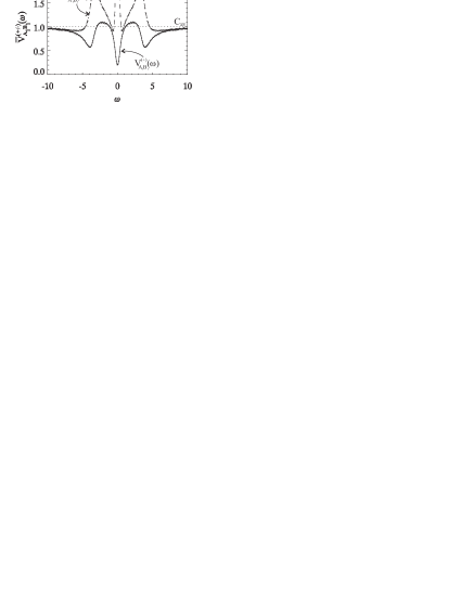
FIG. 4.: Photon number spectra $\bar{V}_{A_{1}B_{1}}^{(\pm)}(\omega)$ for the parameters in Fig. 3 and $J_{1}=3.0$, $\Delta=0$ and $E=3.275$, on the lower branch just before a bistable turning point. Lines show analytical results while points are numerical results. The shot-noise level is indicated with $C_{SN}$.

A $\gamma$ small

First we consider the case where $\gamma$ is small and good nonclassical correlations in the FH fields are expected ($\bar{V}_{A_{1}}(\omega)\simeq\gamma/[1+\gamma]$ close to self-pulsing transitions) [5]. For $\gamma=0.1$ we observed the strongest violations of the quantum limit close to bistable turning points. An example is shown in Fig. 4 located in the bistable region of Fig. 3, and the system is set on the lower branch of the bistable curve just before the right turning point. The dimer spectrum of the sum of the FH fields shows a near Lorentzian dip in the region of $\omega=0$ that goes down to $\bar{V}_{A_{1}B_{1}}^{(+)}(\omega)\simeq 0.2$, implying strong twin-beam correlations, while the FH difference shows excess noise here. Taking $\gamma$ even smaller we were able to get $\bar{V}_{A_{1}B_{1}}^{(+)}(\omega)$ very close to zero in the presence of bistable turning points, a behavior similar to the $\gamma/(1+\gamma)$ behavior observed in the SHG monomer close to self-pulsing transitions. The excellent correlations are only seen close to the bistable transition, taking e.g. $E=3.2$ for the parameters in Fig. 4, the minimum of the spectrum is $\bar{V}_{A_{1}B_{1}}^{(+)}(\omega)\simeq 0.35$. Returning to Fig. 4, at $\omega\simeq 4$ the FH sum spectrum again shows nonclassical correlations of approximately 60% of the shot-noise limit. The frequency almost coincides with the frequency of the Hopf instability that is suppressed here; the eigenvalue with the largest real part is the bistable one while the eigenvalues with more negative real parts have ${\mathrm{I}m}(\lambda)\simeq 3.6$.

Here it is relevant to mention that bistability is also present in the SHG monomer [38, 43] (as Eq. (52) indicates this requires nonzero detunings with equal sign), and to the best of our knowledge nobody has here investigated the quantum behavior. Let us write the detunings of the SHG monomer as $\bar{\Delta}_{j}$. Due to the invariance of the symmetric steady state solutions when $\bar{\Delta}_{j}=\Delta_{j}-J_{j}$ we can obtain the same bistable state investigated in Fig. 4 in the SHG monomer by setting $\bar{\Delta}_{1}=-3.0$ and $\bar{\Delta}_{2}=-1.0$. The spectrum $\bar{V}_{A_{1}}(\omega)$ displays here exactly the same behavior as $\bar{V}_{A_{1}B_{1}}^{(+)}(\omega)$ in Fig. 4, so also in the SHG monomer perfect anti-bunching behavior may be obtained in the small $\gamma$ limit. Generally, the dimer spectra $\bar{V}_{A_{i}B_{i}}^{(+)}(\omega)$ can be reproduced by the monomer spectra $\bar{V}_{A_{i}}(\omega)$ when taking $\bar{\Delta}_{j}=\Delta_{j}-J_{j}$. This is not valid, however, close to a transition to asymmetric states, and also the spectra $\bar{V}_{A_{i}B_{i}}^{(-)}(\omega)$ have no equivalents in the no-coupling intensity correlations.

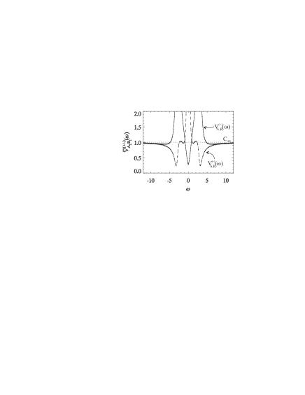
FIG. 5.: Photon number spectra $\bar{V}_{A_{1}B_{1}}^{(\pm)}(\omega)$ for the parameters in Fig. 3, $J_{1}=2.0$, $\Delta=0$ and $E=2.3$. Lines show analytical results while points are numerical results. The shot-noise level is indicated with $C_{SN}$.

In the self-pulsing region of Fig. 3 it is possible to obtain good correlations if the system is set close to the bistable area. The spectra in Fig. 5 are for a pump value where both the bistable and the self-pulsing eigenvalues are of approximately the same strength, and the plot shows that the dimer spectrum of the FH difference have strong noise suppression for nonzero $\omega$, that originates from the self-pulsing instability setting in at $E_{\mathrm{S}P}=4.7$. Also the sum shows strong noise suppression now at $\omega=0$, caused by the proximity of the bistable area which gives rise to an eigenvalue with ${\mathrm{I}m}(\lambda)=0$ that never has ${\mathrm{R}e}(\lambda)>0$. The good correlations observed here are apparently a result of a competition between the bistable state and the emerging self-pulsing instability, that eventually dominates for higher pump levels. When the self-pulsing threshold is approached, the nonclassical behavior is less pronounced. This does not necessarily mean that nonclassical states are not present here, but probably that the intensity is the wrong observable in which to observe nonclassical correlations here. Such a case was observed in the SHG monomer, where it was found that detuning of the system makes the squeezing ellipse turn so the best squeezing is no longer observed in the amplitude quadrature [42].

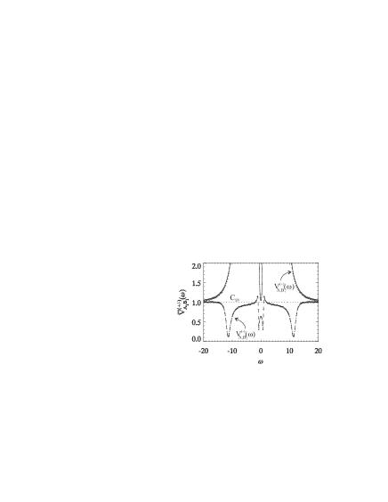
FIG. 6.: Photon number spectra for $\Delta_{1}=\Delta_{2}=1.1$ and $\gamma=0.1$, $J_{1}=20.0$, $J_{2}=1$ and $E/E_{\mathrm{s}ym}=0.97$. Lines show analytical results while points are numerical results. The shot-noise level is indicated with $C_{SN}$.

When detuning is introduced, the system can become asymmetrically unstable for certain couplings as was shown in Fig. 3. Generally, the asymmetric instability shows sub-Poissonian twin-beam correlations in the dimer FH difference spectrum, which is especially pronounced when $J_{1}\gg J_{2}$ where almost perfect anti-bunching was observed. In Fig. 6 the dimer spectra $\bar{V}_{A_{1}B_{1}}^{(\pm)}(\omega)$ are shown for $\Delta=1.1$, $J_{1}=20$ and $J_{2}=1$, taken close to the symmetric transition $E_{\mathrm{s}ym}$, and intensity correlations until 8% of the shot-noise limit is seen in the FH difference correlations at nonzero $\omega$. By carefully selecting the parameters we were even able to see correlations until 3% of the shot-noise level, which underlines that excellent nonclassical correlations are observed here. This result is quite robust; good sub-Poissonian correlations are observed also further below the transition as well as for considerably lower values of the FH coupling strength, while the peaked structure around $\omega=0$ is quite sensitive to the pump level since it is not seen taking the system even closer to $E_{\mathrm{s}ym}$. We note from Fig. 3 the presence of the self-pulsing instability for the parameters chosen, and even if quite good correlations are observed inside the large asymmetric area for $J_{1}$ large, the best results are obtained close to the self-pulsing regions. Again this shows that two competing instabilities appear to give rise to strong nonclassical correlations. We note finally that the frequency $\omega\simeq 11$, where the best correlations in Fig. 6 are observed, almost coincides with the frequency of the self-pulsing eigenvalue that is damped the most. Thus, paradoxically, in this case the least dominating eigenvalue is determining the frequency of the strong correlations.

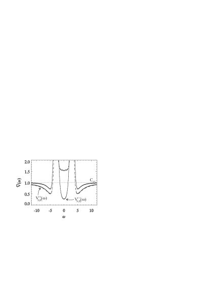
FIG. 7.: Photon number spectra on resonance and for $\gamma=1$ and $J_{1}=4.0$, $J_{2}=1.0$ and $E/E_{\mathrm{S}P}=0.95$. Lines show analytical results while points are numerical results. The shot-noise level is indicated with $C_{SN}$.

B $\gamma=1$

Setting the loss rates to be identical, $\gamma=1$, the self-pulsing instability gives rise to strong nonclassical correlations all the way to the transition to the self-pulsing state, while the bistable transition displays only weak violations. As an example of the self-pulsing correlations Fig. 7 displays selected spectra for the dimer correlations. The sum of the SH fields displays strong correlations at $\omega=0$, which goes to 25% of the shot-noise limit when $E\rightarrow E_{\mathrm{S}P}$, a result that can also be found in the SHG monomer by introducing equivalent detunings. Also the dimer FH difference correlations are strong; for nonzero $\omega$ correlations around 50% of the shot-noise limit are seen.

C $\gamma$ large

For large $\gamma$ the SHG monomer predicts strong shot-noise violations in the SH spectrum at the self-pulsing threshold [5] ($\bar{V}_{A_{2}}(\omega)\simeq(1+\gamma)^{-1}$ close to self-pulsing transitions), and for the dimer similar levels of correlations can be obtained close to the self-pulsing transition. As an example of the behavior Fig. 8 shows highly nonclassical twin-beam correlations in the dimer spectrum for the sum of the SH intensities. For the selected parameters we observe also sub-Poissonian behavior in $\bar{V}_{A_{2}B_{2}}^{(-)}(\omega)$, which, in contrast to $\bar{V}_{A_{2}B_{2}}^{(+)}(\omega)$, cannot be observed in the SHG monomer with equivalent detunings. Although asymmetric areas were found for nonzero detunings, only weak sub-Poissonian correlations were observed there in the difference of the SH fields (the sum correlations still show strong sub-Poissonian correlations here, as expected from the SHG monomer predictions).

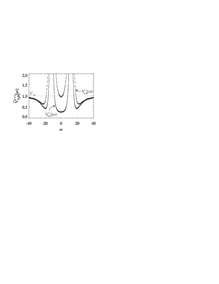
FIG. 8.: Photon number spectra on resonance and for $\gamma=10$ and $J_{1}=6.0$, $J_{2}=2.0$, and $E/E_{\mathrm{S}P}=0.95$. Lines show analytical results while points are numerical results. The shot-noise level is indicated with $C_{SN}$.

VI Summary and discussion

In this paper we have proposed a model we denote the quantum optical dimer for studying the effects of a simple mode coupling in a cavity. The model consisted of two $\chi^{(2)}$ nonlinear waveguides in a cavity, with coupling between them from evanescent overlapping waves that was assumed weak and linear. We chose to restrict ourselves to investigating nonclassical correlations, and hence derived the nonlinear quantum equations of evolution for the system, resulting in a set of stochastic Langevin equations.

Using a linearized analysis we showed that the system for low pump levels allowed a symmetric state to be stable, where both waveguides are in the same stable state. Depending on the system parameters this state destabilized into a self-pulsing state, where temporal oscillations are observed, or bistable solutions in the steady states occurred. For some parameters, the symmetric steady state lost stability in favor of an asymmetric steady state, in which the two waveguides has different steady state solutions.

We investigated the effects of the quantum noise present in the system by calculating two-time intensity correlation spectra of the output fields. It was shown that sub-Poissonian correlations were present in the system, especially when considering the sum or difference of the field intensities from each waveguide implying strong twin-beam correlations. This nonclassical anti-bunching effect is a true manifestation of a quantum behavior and was observed mainly in three cases:

• Close to bistable turning points the strongest violations of the classical limit were observed in the spectrum at $\omega=0$, corresponding to correlations at infinite time. In the limit of $\gamma\ll 1$ perfect noise suppression could be obtained in the sum of the FH intensities, resulting in perfect twin-beam behavior. This was also observed in the single waveguide model, when equivalent detunings were introduced.

• Close to threshold for self-pulsing behavior strong twin-beam correlations were observed both at $\omega=0$ and also at values of $\omega$ coinciding with the oscillation frequency of the emerging instability. Thus, the correlations here anticipate the behavior above the threshold analogously to the idea of a quantum image [44], where the spatial modulations are encoded in the correlations below threshold while the average intensity remains homogeneous.

• Excellent sub-Poissonian correlations were observed close to transitions from symmetric to asymmetric steady states, which is a wholly unique transition to the dimer. This instability is closely related to the near-field of a modulationally unstable system in presence of diffraction; the dimer sites could be thought of as neighboring near-field pixels. Variances down to 3% of the shot-noise level were observed in the the difference of the FH fields, implying nearly perfect twin-beam behavior. The correlations were particularly strong when the FH coupling strength was much larger than the SH and when the FH loss rate was much larger than the SH loss rate. These results indicate that strong near-field correlations can be observed in SHG with diffraction close to a modulational instability, which to our knowledge has not been investigated yet.

It is worth noting that the twin-beam correlations reported here were all originating from the dimer coupling across the waveguides; while each field was created individually from the nonlinear interaction in the corresponding waveguide, the coupling between the waveguides gave rise to the strong nonclassical twin-beam correlations. Hence, the nonclassical correlations arise not because the photons are twins, but rather because they are “brothers”.

Common for all these cases was that distinctively strong nonclassical correlations were observed in parameter regimes where two types of instabilities were competing. This was observed in self-pulsing areas close to bistable and asymmetric regimes, and also in asymmetric areas close to bistable and self-pulsing regimes. These enhanced correlations from competing instabilities has to the best of our knowledge not been reported before.

We showed that the relative input mirror loss rate $\gamma=\gamma_{2}/\gamma_{1}$ between the SH and FH fields had a strong influence on the sub-Poissonian behavior, as was previously shown by Collett and Walls [5] in the SHG monomer. For small $\gamma$ the strongest nonclassical states were mainly observed in the FH fields while for large $\gamma$ they were mainly observed in the SH fields. Since the photon life times in the cavity are inversely proportional to the loss rates of the input mirror, the time spent in the cavity is decisive for the level of nonclassical correlations of the output fields; the field with the shortest time spent in the cavity displays the strongest nonclassical correlations. The fact that a long interaction time tends to destroy the nonclassical correlations have also been observed in propagation setups, specifically Olsen et al. [45] showed that in propagation SHG the presence of quantum fluctuations caused a dramatic revival of the FH after a certain propagation length, causing the variance to go above shot-noise level.

We stress that the results presented here were very robust to changes in the parameters. Thus, large parameters areas exist where strong nonclassical behavior can be seen. This is especially important to stress for the coupling parameters, since they are not so easily controlled experimentally.

We investigated only the symmetric state of the system, and a future study of the stability, dynamics and nonclassical properties of the asymmetric states is relevant. In this context we should also mention that the coupling between the waveguides chosen here was conservative (imaginary coupling in the Langevin equations) while it could also have been dissipative (real) or a combination (complex). This highly depends on the actual setup, and a future study should include the possibility of a general complex coupling.

VII Acknowledgements

Financial support from Danish National Science Research Council grant no. 9901384 is gratefully acknowledged. We thank Pierre Scotto, Roberta Zambrini, Peter Lodahl, Jens Juul-Rasmussen, Mark Saffman and Ole Bang for fruitful discussions. Y.G. thanks MIDIT and Informatics and Mathematical Modelling at the Technical University of Denmark for financial support.

A The quantum-to-classical correspondence

In this section we show how the master equation (6) is converted into an equivalent partial differential equation by expanding the density matrix in coherent states weighted by a quasi-probability distribution [28, 29]. In this distribution the operators are replaced by equivalent $c$-numbers, where the particular correspondence between these depends on the ordering of the operators. In the case where only up to second order derivatives appear in the corresponding partial differential equation, the equation is on Fokker-Planck form allowing equivalent sets of stochastic Langevin equations to be found.

We are now left with a choice of probability distribution, be it either the $P$, Wigner or $Q$ distribution giving normal, symmetric or anti-normal averages, respectively. The aim of this paper is to calculate two-time correlation spectra outside the cavity, and in order to do this most conveniently, the moments of the intracavity fields must be time and normally ordered, cf. the discussion in Sec. IV. Since the $P$-representation will immediately give the time and normally ordered averages needed, this is the favorable representation in this context. As will be explained later we use the Wigner representation for the numerical simulations, and therefore we now provide a general way of deriving the QPD equations.

The approach we use is to introduce a characteristic function

$$\chi(z)={\mathrm{T}r}[\hat{D}(z)\hat{\rho}],$$ (A1)

so $\chi$ is the trace over a displacement operator $\hat{D}(z)$ acting on the density matrix [i.e. the expectation value of $\hat{D}(z)$]. The choice of ordering now amounts to choosing the ordering of $\hat{D}(z)$. In the symmetric ordering

$$\hat{D}_{s}(z)=e^{z\hat{A}^{\dagger}-z^{*}\hat{A}},$$ (A2)

where $z$ is a complex number describing the amplitude of a coherent field, and $\hat{A}$ is a boson operator. The normally ordered displacement operator is

$$\hat{D}_{n}(z)=e^{z\hat{A}^{\dagger}}e^{-z^{*}\hat{A}},$$ (A3)

and the anti-normally ordered displacement operator is

$$\hat{D}_{a}(z)=e^{-z^{*}\hat{A}}e^{z\hat{A}^{\dagger}}.$$ (A4)

The QPD is now given as a Fourier transform of the characteristic function

$$W(\alpha)=\int d^{2}z\chi(z)e^{z^{*}\alpha-z\alpha^{*}},$$ (A5)

where the integration measure $d^{2}z$ means integration over the entire complex plane. From this relation an equivalence between operators and $c$-numbers has been established as $\hat{A}\leftrightarrow\alpha$ and $\hat{A}^{\dagger}\leftrightarrow\alpha^{*}$. The $c$-number averages may now be calculated as, e.g.,

$$\langle\alpha^{*}\alpha\rangle=\int d^{2}\alpha W(\alpha)\alpha^{*}\alpha,$$

and obviously since the operator ordering determines the specific form of $W(\alpha)$ from Eq. (A5), this in turn implies that the $c$-number averages also are influenced by the choice of ordering.

From differentiating Eq. (A1) with respect to time we get

$$\frac{\partial\chi(z)}{\partial t}={\mathrm{T}r}\left(\hat{D}(z)\frac{\partial\hat{\rho}}{\partial t}\right),$$ (A6)

with $\partial_{t}\hat{\rho}$ being governed by the master equation (6), and we have used that in the Schrödinger picture the operators [here $\hat{D}(z)$] are independent of time. The approach is now to differentiate $\hat{D}(z)$ with respect to e.g. $z$ and rearrange to get

$$\hat{A}^{\dagger}\hat{D}_{s}(z)=\left(\frac{\partial}{\partial z}+\frac{z^{*}}{2}\right)\hat{D}_{s}(z).$$ (A7)

The right hand side of Eq. (A6) is evaluated using Eq. (A7) and the similar other expressions. Eq. (A6) is then Fourier transformed according to Eq. (A5), assuming the characteristic function is well behaved, to finally give the equation governing the time evolution of $W(\alpha)$.

Choosing the normally ordered displacement operator given by Eq. (A3) the equation for the Glauber-Sudarshan $P$-representation is derived, which is on Fokker-Planck form. However, due to problems with negative diffusion in quantum optics the generalized $P$-distributions [46, 47] are normally used instead, where the problems are surpassed by doubling the phase space. We will use the positive $P$-representation, which can be derived by replacing all $\alpha_{j}^{*}\rightarrow\alpha_{j}^{\dagger}$ and $\beta_{j}^{*}\rightarrow\beta_{j}^{\dagger}$ in the Fokker-Planck equation of the Glauber-Sudarshan $P$-representation. This means that $\alpha_{j}^{\dagger}$ is now an independent complex quantity instead of being the complex conjugate of $\alpha_{j}$. The Fokker-Planck equation using the positive $P$-representation corresponding to the master equation (6) is then

$$\frac{\partial W_{n}({\mathbf{x}})}{\partial t} = \Bigg{\{}\frac{\partial}{\partial\alpha_{1}}\left[\alpha_{1}(\gamma_{1}-i\delta_{1})+iJ_{1}\beta_{1}-\kappa\alpha_{1}^{\dagger}\alpha_{2}-\mathcal{E}_{\mathrm{p},a}\right]$$ (A8)

$$+ \frac{\partial}{\partial\alpha_{1}^{\dagger}}\left[\alpha_{1}^{\dagger}(\gamma_{1}+i\delta_{1})-iJ_{1}\beta_{1}^{\dagger}-\kappa\alpha_{1}\alpha_{2}^{\dagger}-\mathcal{E}_{\mathrm{p},a}^{*}\right]$$ (A9)

$$+ \frac{\partial}{\partial\alpha_{2}}\left[\alpha_{2}(\gamma_{2}-i\delta_{2})+iJ_{2}\beta_{2}+\frac{\kappa}{2}{\alpha_{1}}^{2}\right]$$ (A10)

$$+ \frac{\partial}{\partial\alpha_{2}^{\dagger}}\left[\alpha_{2}^{\dagger}(\gamma_{2}+i\delta_{2})-iJ_{2}\beta_{2}^{\dagger}+\frac{\kappa}{2}{\alpha_{1}^{\dagger}}^{2}\right]$$ (A11)

$$+ \frac{\partial}{\partial\beta_{1}}\left[\beta_{1}(\gamma_{1}-i\delta_{1})+iJ_{1}\alpha_{1}-\kappa\beta_{1}^{\dagger}\beta_{2}-\mathcal{E}_{\mathrm{p},b}\right]$$ (A12)

$$+ \frac{\partial}{\partial\beta_{1}^{\dagger}}\left[\beta_{1}^{\dagger}(\gamma_{1}+i\delta_{1})-iJ_{1}\alpha_{1}^{\dagger}-\kappa\beta_{1}\beta_{2}^{\dagger}-\mathcal{E}_{\mathrm{p},b}^{*}\right]$$ (A13)

$$+ \frac{\partial}{\partial\beta_{2}}\left[\beta_{2}(\gamma_{2}-i\delta_{2})+iJ_{2}\alpha_{2}+\frac{\kappa}{2}\beta_{1}^{2}\right]$$ (A14)

$$+ \frac{\partial}{\partial\beta_{2}^{\dagger}}\left[\beta_{2}^{\dagger}(\gamma_{2}+i\delta_{2})-iJ_{2}\alpha_{2}^{\dagger}-\frac{\kappa}{2}{\beta_{2}^{\dagger}}^{2}\right]$$ (A15)

$$+ \frac{\kappa}{2}\Big{[}\frac{\partial^{2}}{\partial\alpha_{1}^{2}}\alpha_{2}+\frac{\partial^{2}}{\partial{\alpha_{1}^{\dagger}}^{2}}\alpha_{2}^{\dagger}$$ (A17)

$$\;\;\;+\frac{\partial^{2}}{\partial\beta_{1}^{2}}\beta_{2}+\frac{\partial^{2}}{\partial{\beta_{1}^{\dagger}}^{2}}\beta_{2}^{\dagger}\Big{]}\Bigg{\}}W_{n}({\mathbf{x}}),$$

where the $c$-number equivalents of the operators are $\{\hat{A}_{j},\hat{A}_{j}^{\dagger}\}\leftrightarrow\{\alpha_{j},\alpha_{j}^{\dagger}\}$ and $\{\hat{B}_{j},\hat{B}_{j}^{\dagger}\}\leftrightarrow\{\beta_{j},\beta_{j}^{\dagger}\}$, and ${\mathbf{x}}$ represents the $c$-number states

$${\mathbf{x}}=\{\alpha_{1},\alpha_{1}^{\dagger},\alpha_{2},\alpha_{2}^{\dagger},\beta_{1},\beta_{1}^{\dagger},\beta_{2},\beta_{2}^{\dagger}\}.$$ (A18)

The numerical simulation of the positive $P$-representation has been reported as very difficult, mainly due to divergent trajectories [48], cf. the discussion in App. B. Therefore we choose to use the Wigner representation for the numerical simulations, obtained by using the symmetric displacement operator (A2). The time evolution of the Wigner distribution is governed by

$$\frac{\partial W_{s}({\mathbf{x}})}{\partial t} = \Bigg{\{}\frac{\partial}{\partial\alpha_{1}}[(\gamma_{1}-i\delta_{1})\alpha_{1}-\kappa\alpha_{1}^{*}\alpha_{2}+iJ_{1}\beta_{1}-\mathcal{E}_{\mathrm{p},a}]$$ (A19)

$$+ \frac{\partial}{\partial\alpha_{2}}[(\gamma_{2}-i\delta_{2})\alpha_{2}+\frac{\kappa}{2}\alpha_{1}^{2}+iJ_{2}\beta_{2}]$$ (A20)

$$+ \frac{\partial}{\partial\beta_{1}}[(\gamma_{1}-i\delta_{1})\beta_{1}-\kappa\beta_{1}^{*}\beta_{2}+iJ_{1}\alpha_{1}-\mathcal{E}_{\mathrm{p},b}]$$ (A21)

$$+ \frac{\partial}{\partial\beta_{2}}[(\gamma_{2}-i\delta_{2})\beta_{2}+\frac{\kappa}{2}\beta_{1}^{2}+iJ_{2}\alpha_{2}]$$ (A22)

$$+ \frac{\gamma_{1}}{2}\left(\frac{\partial^{2}}{\partial\alpha_{1}\partial\alpha_{1}^{*}}+\frac{\partial^{2}}{\partial\beta_{1}\partial\beta_{1}^{*}}\right)$$ (A23)

$$+ \frac{\gamma_{2}}{2}\left(\frac{\partial^{2}}{\partial\alpha_{2}\partial\alpha_{2}^{*}}+\frac{\partial^{2}}{\partial\beta_{2}\partial\beta_{2}^{*}}\right)$$ (A24)

$$+ \frac{\kappa}{4}\left(\frac{\partial^{3}}{\partial\alpha_{1}^{2}\partial\alpha_{2}^{*}}+\frac{\partial^{3}}{\partial\beta_{1}^{2}\partial\beta_{2}^{*}}\right)+c.c.\Bigg{\}}W_{s}({\mathbf{x}}),$$ (A25)

where the $c$-number equivalents of the operators are $\{\hat{A}_{j},\hat{A}_{j}^{\dagger}\}\leftrightarrow\{\alpha_{j},\alpha_{j}^{*}\}$ and $\{\hat{B}_{j},\hat{B}_{j}^{\dagger}\}\leftrightarrow\{\beta_{j},\beta_{j}^{*}\}$ and

$${\mathbf{x}}=\{\alpha_{1},\alpha_{1}^{*},\alpha_{2},\alpha_{2}^{*},\beta_{1},\beta_{1}^{*},\beta_{2},\beta_{2}^{*}\}.$$ (A26)

Due to the third order derivatives Eq. (A19) is not on Fokker-Planck form, a problem we address in App. B. Note that the $+c.c.$ term (denoting the complex conjugate) at the end applies to the entire equation.

The connection from the QPD equations to the stochastic Langevin equations can be made if the QPD equation is on Fokker-Planck form, which for a system with $m$ $c$-number states $x_{j}$ is [29]

$$\frac{\partial W({\mathbf{x}})}{\partial t}=\Big{\{} -\sum_{j=1}^{m}\frac{\partial}{\partial x_{j}}A_{j}({\mathbf{x}})$$ (A28)

$$+\frac{1}{2}\sum_{j,k=1}^{m}\frac{\partial^{2}}{\partial x_{j}\partial x_{k}}D_{jk}({\mathbf{x}})\Big{\}}W({\mathbf{x}}),$$

Using Ito rules for stochastic integration the equivalent set of Langevin equations is

$$\frac{\partial x_{j}}{\partial t}=A_{j}({\mathbf{x}})+w_{j}(t),$$ (A29)

where $w_{j}(t)$ are Gaussian white noise terms, delta correlated in time according to the diffusion matrix ${\mathbf{D}}$

$$\langle w_{j}(t)w_{k}(t^{\prime})\rangle=D_{jk}({\mathbf{x}})\delta(t-t^{\prime}).$$ (A30)

We note that if ${\mathbf{D}}$ depends on ${\mathbf{x}}$ the noise is labeled multiplicative which is the case for the positive-$P$ Eq. (A17), otherwise it is additive as it is for the Wigner Eq. (A19).

B Numerical simulations

The choice of using the Wigner representation for the numerical simulations is not immediately apparent, since it involves an approximation that is not necessary if the $P$ or the $Q$-representation are used. The advantage of the truncated Wigner Langevin equations (II) is that the noise is additive, as opposed to the the multiplicative noise of the $Q$-representation (where the noise for the quantum SHG model poses serious limits on the parameter space [10]) and the $P$-representation. For the $P$-representation we are forced to use the generalized representations in order to avoid negative diffusion in the Fokker-Planck equation. Since this choice implies doubling of the phase space, the $c$-numbers $\alpha_{j}$ and $\alpha_{j}^{\dagger}$ are no longer each others complex conjugate (only on average) and the respective noise terms are not correlated to each other, cf. Eq. (II). This may lead to divergent trajectories where the convergence is extremely slow, and is the major reason for us avoiding a numerical implementation of the positive-$P$ equations. The Wigner equations, on the other hand, have no problems in this direction.

The drawbacks to using the Wigner equations are first of all that we have to neglect the third order terms of the Wigner QPD equation (A19) to get it on Fokker-Planck form so the equivalent Langevin equations (A29) may be obtained. It is uncertain what the implications of this approximation are, however in many cases no major differences have been observed between simulations of the truncated Wigner equations compared to exact positive-$P$ or $Q$ equations [42, 10]. On the other hand in Ref.[32] so-called quantum jump processes in the degenerate OPO above threshold are shown to produce significant differences between the truncated Wigner and the positive $P$-representation. In our case the third order terms are $O(\kappa^{4})$ while the other terms are $O(\kappa^{2})$ or lower. And because of the weak nonlinear coupling the effect of the third order terms is weak, justifying the truncation. Another drawback to the Wigner representation is that the intracavity averages are symmetrically ordered, and these cannot be rewritten to time and normal ordering since the intracavity commutator relations are not known for $t\neq t^{\prime}$ (only the output fields have well defined correlations here). This means that in order to compute the output fields at a given time $t$ we are forced to use Eq. (53), and here the Gaussian white noise part of the input field is an ill-defined instantaneous quantity. The output fields of the numerics are calculated by using the fact that although the derivative and instantaneous value of a stochastic term are ill-defined, the integral is well-defined. By integrating over a time window (which we denote $\Delta\tau$) and calculating the average, as described in Ref. [49], we may obtain the output fields from Eq. (53).

We use the Heun method [50] to numerically solve the Langevin equations for the intracavity fields and to evaluate the output fields, and a random number generator [51] for generating the Gaussian noise terms. The time step was set to $\Delta t=0.001$ and checked to be stable. The size of the time window for calculating the output fields was varied between $\Delta\tau=40\Delta t-200\Delta t$ according to the resolution needed for the individual spectra. Finally, we set the noise strength parameter $n_{s}=10^{8}$, which is a typical value for the cavity configuration considered here [52].

The averages calculated using the output fields of the numerics correspond to symmetrically ordered averages since they are calculated from the Wigner Langevin equations. In order to relate these averages to the normally ordered averages of the spectra in Sec. IV, the output commutator relations (54) are used to rewrite the output correlations. The classical steady states of the output fields are found from the average of Eq. (53) as

$${\mathcal{F}}_{1,{\mathrm{o}ut}} = \sqrt{2\gamma_{1}}{\mathcal{F}}_{1}+{\mathcal{E}_{\mathrm{p}}}/\sqrt{2\gamma_{1}}$$ (B2)

$${\mathcal{F}}_{2,{\mathrm{o}ut}} = \sqrt{2\gamma_{2}}{\mathcal{F}}_{2},\quad{\mathcal{F}=A,B},$$ (B3)

by taking the input fluctuation to be zero on average. Assuming that the output fields are fluctuating around the output steady states

$$\Delta\hat{A}_{j,{\mathrm{o}ut}}=\hat{A}_{j,{\mathrm{o}ut}}-{\mathcal{A}}_{j,{\mathrm{o}ut}},$$ (B4)

we introduce the photon number fluctuation operator for waveguide A as

$$\Delta\hat{N}_{j,{\mathrm{o}ut}}^{A}(t) \equiv \hat{N}_{j,{\mathrm{o}ut}}^{A}(t)-\langle\hat{N}_{j,{\mathrm{o}ut}}^{A}\rangle_{s}$$ (B5)

$$\simeq {\mathcal{A}}_{j,{\mathrm{o}ut}}\Delta\hat{A}_{j,{\mathrm{o}ut}}^{\dagger}(t)+{\mathcal{A}}_{j,{\mathrm{o}ut}}^{*}\Delta\hat{A}_{j,{\mathrm{o}ut}}(t),$$ (B6)

with subscript $s$ to indicate that the average is symmetric and we have neglected higher order terms in the fluctuations. Using this expression, the two-time correlation function (60) is with a symmetric ordering of the operators to leading order

$$C_{A_{j}B_{k}}^{(\pm)}(\tau)\simeq\langle \Delta\hat{N}^{A}_{j,{\mathrm{o}ut}}(t)\pm\Delta\hat{N}^{B}_{k,{\mathrm{o}ut}}(t),$$ (B8)

$$\Delta\hat{N}^{A}_{j,{\mathrm{o}ut}}(t+\tau)\pm\Delta\hat{N}^{B}_{k,{\mathrm{o}ut}}(t+\tau)\rangle_{s}.$$

The symmetric $c$-number correlations of the output field fluctuations are now calculated in the numerical simulations of the dimensionless Wigner Langevin equations (II) as $\langle\Delta{\mathbf{w}}^{s}(0),[\Delta{\mathbf{w}}^{s}(\tau)]^{T}\rangle_{s}$ where

$$\Delta{\mathbf{w}}^{s}=\left[\Delta{A_{1}},\Delta A_{1}^{*},\Delta{A_{2}},\Delta A_{2}^{*},\Delta{B_{1}},\Delta B_{1}^{*},\Delta{B_{2}},\Delta B_{2}^{*}\right]^{T}.$$ (B9)

The spectral matrix ${\mathbf{S}}^{s}(\omega)$ of fluctuations is now straightforwardly given by the Fourier transform of these correlations, and the correlations (B8) may now be calculated in the same manner as shown in Sec. IV with the shot-noise level

$$C_{SN}=(|{\mathcal{A}}_{{\mathrm{o}ut},j}|^{2}+|{\mathcal{B}}_{{\mathrm{o}ut},k}|^{2})n_{s}^{-1},$$ (B10)

using that the normalization of the output fields are the same as the one taken for the input fields in Eq. (34). Note that the shot noise level, here expressed in the symmetric averages in the Wigner Langevin equation, is identical to the shot-noise level expressed in averages from the positive-$P$ equations (80), since $|{\mathcal{A}}_{{\mathrm{o}ut},j}|^{2}=2\bar{\gamma}_{j}\bar{I}_{j}$. This is due to the approximation made in Eq. (B6).

In the analytical treatment in Sec. IV we used that in the spectral matrix ${\mathbf{S}}(\omega)$ certain symmetries are present, so in fact only approximately one third of the 64 correlations were needed to obtain the results presented there. In a numerical simulation this is only approximately valid in the limits of long integration times and large correlation times. Much better results are obtained faster if the spectra are calculated directly from the full $8\times 8$ matrix ${\mathbf{S}}^{s}(\omega)$.

REFERENCES

- [1] L. A. Lugiato, M. Brambilla, and A. Gatti, in Advances in Atomic, Molecular and Optical Physics, edited by B. Bederson and H. Walther (Academic, Boston, 1999), Vol. 40, p. 229.
- [2] Squeezed states of the electromagnetic field, edited by H. J. Kimble and D. F. Walls (Special issue of J. Opt. Soc. Am. B 4, 1449, 1987).
- [3] L. Davidovich, Rev. Mod. Phys. 68, 127 (1996).
- [4] P. D. Drummond, K. J. McNeil, and D. F. Walls, Opt. Acta 28, 211 (1981).
- [5] M. J. Collett and D. F. Walls, Phys. Rev. A 32, 2887 (1985).
- [6] R. E. Slusher, L. W. Hollberg, B. Yurke, J. C. Mertz, and J. F. Valley, Phys. Rev. Lett. 55, 2409 (1985).
- [7] S. F. Pereira, M. Xiao, H. J. Kimble, and J. L. Hall, Phys. Rev. A 38, 4931 (1988).
- [8] A. C. Scott and P. L. Christiansen, Phys. Scripta 42, 257 (1990).
- [9] N. P. Pettiaux, P. Mandel, and C. Fabre, Phys. Rev. Lett. 66, 1838 (1991).
- [10] M. Bache, P. Scotto, R. Zambrini, M. San Miguel, and M. Saffman, Phys. Rev. A 66, 013809 (2002).
- [11] S. Reynaud, C. Fabre, and E. Giacobino, J. Opt. Soc. Am. B 4, 1520 (1987).
- [12] A. Heidmann, R. J. Horowicz, S. Reynaud, E. Giacobino, C. Fabre, and G. Camy, Phys. Rev. Lett. 59, 2555 (1987).
- [13] L. A. Lugiato and G. Strini, Opt. Commun. 41, 67 (1982).
- [14] A. Eschmann and R. J. Ballagh, Phys. Rev. A 60, 559 (1999).
- [15] L. Fabiny, P. Colet, R. Roy, and D. Lenstra, Phys. Rev. A 47, 4287 (1993).
- [16] C. Serrat, M. C. Torrent, J. Garcia-Ojalvo, and R. Vilaseca, Phys. Rev. A 64, 041802(R) (2001).
- [17] C. Serrat, M. C. Torrent, J. Garcia-Ojalvo, and R. Vilaseca, Phys. Rev. A 65, 053815 (2002).
- [18] A. Z. Khoury, Phys. Rev. A 60, 1610 (1999).
- [19] T. Peschel, U. Peschel, F. Lederer, and B. A. Malomed, Phys. Rev. E 55, 4730 (1997).
- [20] O. Bang, P. L. Christiansen, and C. B. Clausen, Phys. Rev. E 56, 7257 (1997).
- [21] J. Perina Jr and J. Perina, in Progress in optics, edited by E. Wolf (Elsevier, Holland, 2000), Vol. 41, p. 361.
- [22] R. Wynar, R. Freeland, D. J. Han, C. Ryu, and D. J. Heinzen, Science 287, 1016 (2000).
- [23] D. J. Heinzen, R. Wynar, P. D. Drummond, and K. V. Kheruntsyan, Phys. Rev. Lett. 84, 5029 (2000).
- [24] P. D. Drummond, K. V. Kheruntsyan, and H. He, Phys. Rev. Lett. 81, 3055 (1998).
- [25] U. V. Poulsen and K. Mølmer, Phys. Rev. A 63, 023604 (2001).
- [26] G. J. Milburn, J. Corney, E. M. Wright, and D. F. Walls, Phys. Rev. A 55, 4318 (1997).
- [27] The model for degenerate optical parametric oscillation is found by simply having the classical pump field in the SH mode, so this term would be .
- [28] D. F. Walls and G. J. Milburn, Quantum Optics (Springer Verlag, Berlin, 1994).
- [29] H. J. Carmichael, Statistical methods in quantum optics 1 (Springer Verlag, Berlin, 1999).
- [30] L. Mandel and E. Wolf, Optical coherence and quantum optics (Cambridge, New York, 1995).
- [31] In fact, in the present model both Ito and Stratonovich rules for interpreting the stochastic integration give identical results.
- [32] P. Kinsler and P. D. Drummond, Phys. Rev. A 43, 6194 (1991).
- [33] If independent control over the detuning is desired a dichroic mirror could be inserted in the cavity, see P. Lodahl, M. Bache, and M. Saffman, Phys. Rev. A 63, 023815 (2001), however this would introduce additional losses, and hence also noise sources, into the system.
- [34] B. E. A. Saleh and M. C. Teich, Fundamentals of photonics (John Wiley, New York, 1991).
- [35] P. Lodahl and M. Saffman, Phys. Rev. A 60, 3251 (1999).
- [36] Alternatively, the coupling can be achieved by launching two identical modes in a bulk crystal. Taking the modes to be Gaussians with waists and a distance apart, the coupling coefficient can be found as an overlap integral of the modes [15]. After normalization the coupling constants become This approach is valid when diffraction can be neglected, which can be achieved by choosing large, typically 100 m or more. In contrast, the width of the waveguides can typically be chosen to 5-10 m. Additionally, it must be stressed in the bulk case that since there is no waveguiding the energy exchange between the spatially overlapping fields may become complicated and beyond the theory presented here.
- [37] P. Lodahl, M. Bache, and M. Saffman, Phys. Rev. A 63, 023815 (2001).
- [38] C. Etrich, U. Peschel, and F. Lederer, Phys. Rev. E 56, 4803 (1997).
- [39] We consider only solutions in the classical subspace of the positive- representation, where .
- [40] C. W. Gardiner and M. J. Collett, Phys. Rev. A 31, 3761 (1985).
- [41] M. D. Reid, Phys. Rev. A 37, 4792 (1988).
- [42] M. K. Olsen, S. C. G. Granja, and R. J. Horowicz, Opt. Commun. 165, 293 (1999).
- [43] C. Etrich, U. Peschel, and F. Lederer, Phys. Rev. Lett. 79, 2454 (1997).
- [44] L. Lugiato and G. Grynberg, Europhys. Lett. 29, 675 (1995).
- [45] M. K. Olsen, R. J. Horowicz, L. I. Plimak, N. Treps, and C. Fabre, Phys. Rev. A 61, 021803 (2000).
- [46] P. D. Drummond and C. W. Gardiner, J. Phys. A 13, 2353 (1980).
- [47] H. P. Yuen and P. Tombesi, Opt. Commun. 59, 155 (1986).
- [48] A. Gilchrist, C. W. Gardiner, and P. D. Drummond, Phys. Rev. A 55, 3014 (1997).
- [49] R. Zambrini, M. Hoyuelos, A. Gatti, P. Colet, L. Lugiato, and M. San Miguel, Phys. Rev. A 62, 063801 (2000).
- [50] M. San Miguel and R. Toral, in Instabilities and Nonequilibrium Structures VI, Nonlinear phenomena and complex systems, edited by E. Tirapegui, J. Martinez, and R. Tiemann (Kluwer Academic Publishers, Dordrecht, 2000), p. 35.
- [51] R. Toral and A. Chakrabarti, Comput. Phys. Commun. 74, 327 (1993).
- [52] M. Bache, unpublished, (2001).