Discrete Wigner functions and the phase space representation of quantum teleportation

Abstract

We present a phase space description of the process of quantum teleportation for a system with an $N$ dimensional space of states. For this purpose we define a discrete Wigner function which is a minor variation of previously existing ones. This function is useful to represent composite quantum system in phase space and to analyze situations where entanglement between subsystems is relevant (dimensionality of the space of states of each subsystem is arbitrary). We also describe how a direct tomographic measurement of this Wigner function can be performed.

2

I Introduction

Quantum teleportation [1] is a scheme by which an unknown quantum state is transported between two parties by only transmitting classical information between them. This remarkable task requires also that the two parties share the two halfs of a composite system prepared in a specific entangled state. In recent years this scheme has been studied in great detail. Interest in teleportation (whose experimental feasibility has also been recently demonstrated in simple systems [2]) is motivated by more than one reason. In fact, teleportation is one of the most remarkable processes requiring the use of entanglement as essential resource [1, 3]. Moreover, teleportation can also be conceived as a primitive for universal quantum computation [4]. In the seminal work of Bennett et al [1] the teleportation of the state of a qbit (a two level system) was described. Shortly afterwards, Vaidman [5] showed how to generalize this method to include systems with a space of states of arbitrary dimensionality. In this way, the idea of teleporting states of systems with continuous variables was first proposed. A concrete analysis of the teleportation of the state of a continuous system (the electromagnetic field) was first discussed by Braunstein and Kimble [6]. In their work, these authors proposed (and later performed [7]) interesting experiments to accomplish teleportation of continuous variables. For this case, it was natural to describe the whole procedure in terms of phase space distributions [8]. However, this is not the case for systems with a finite dimensional Hilbert space, where the use of the phase space representation is not so common. The description of the usual teleportation protocol in phase space has been recently presented by Koniorczyk, Buzek and Jansky [9] using the discrete version of Wigner functions originally introduced by Wooters [10]. This approach, as mentioned in [9], can only be used when the dimension of the Hilbert space of the system to be teleported is a prime number. In this paper we extend the results presented in [9] to the case where the space of states has arbitrary dimensionality. For this purpose we use a different definition for the discrete Wigner function that turns out to be very convenient to analyze situations where entanglement between subsystems of arbitrary dimensionality is an important issue.

Several methods exist to represent the quantum state of a system with an $N$ dimensional Hilbert space in phase space. As mentioned above, Wooters introduced a discrete version of the Wigner function that has all the desired properties only when $N$ is a prime number[10]. His phase space is an $N\times N$ grid (if $N$ is prime) and a Cartesian product of such spaces corresponding to prime factors of $N$ in the most general case. On the other hand, a different approach to define a Wigner function for a system with an $N$ dimensional Hilbert space was introduced by Leonhardt [11] that rediscovered results previously used by Hannay and Berry [12] and others. This method, that has the property of being well defined for arbitrary values of $N$, was used in several contexts [13, 14] and recently applied to analyze the phase space representation of quantum computers and algorithms [15, 16]. In this case, the phase space is constructed as a grid of $2N\times 2N$ points where the state is represented in a redundant manner (only $N\times N$ of them are truly independent). In this paper, we use a hybrid approach allowing us to capture the most useful features of both Wooters and Leonhardt methods. Thus, to represent a quantum state of a bipartite system we use, following Wooters, a phase space which is a Cartesian product of two grids. Each one of these grids has, as it does in Leonhardt approach, $2N_{i}\times 2N_{i}$ points (where $N_{i}$ is the dimensionality of the Hilbert space of the $i$–th subsystem).

The paper is organized as follows: In Section II we first review the usual approach to define Wigner functions for systems with an $N$ dimensional Hilbert space. Then we introduce a convenient generalization that can be adopted in order to analyze bipartite (or multi–partite) systems. We discuss some general properties of the Wigner function and analyze the phase space representation of a family of entangled states (generalized Bell–EPR states). In Section 3 we show how to describe teleportation of the quantum state of a system with an $N$ dimensional Hilbert space using the Wigner function. In Section IV we describe the procedure by which a direct measurement of the Wigner function of a composite system can be done. In Section V we summarize our conclusions.

II Phase space representation of composite quantum systems

We describe here the formalism of Wigner functions to represent a composite quantum system in phase space. For simplicity, we consider the composite system to be formed by subsystems each one of which has an $N$ dimensional Hilbert space We first describe the properties of discrete Wigner functions for one of the subsystems and later discuss the phase space representation of the composite system. It is clear that one can always split a system into subsystems in many ways. For example, when $N$ is a composite number one can choose to separate each subsystem into even smaller subsystems each one of which has a space of states with the dimensionality of the prime factors of $N$. Adopting this description is simply a matter of physical convenience. Here, we assume that the $N$ dimensional subsystems are the relevant elementary components and that, in some physically interesting regime, the entanglement between them can be manipulated.

A Discrete Wigner functions

To represent the quantum state in phase space we must first define the notions of position and momentum. To do this, we introduce a basis of the Hilbert space $B_{x}=\{|n\rangle,n=0,\ldots,N-1\}$ which we arbitrarily interpret as the position basis (with periodic boundary conditions: $|n+N\rangle=|n\rangle$). Given the position basis $B_{x}$, we introduce the conjugate momentum basis $B_{p}=\{|k\rangle,k=0,\ldots,N-1\}$ by means of the discrete Fourier transform. The states of $B_{p}$ can be obtained from those of $B_{x}$ as

$$|k\rangle={1\over\sqrt{N}}\sum_{n}\exp(i2\pi nk/N)|n\rangle.$$ (1)

As in the continuous case, position and momentum are related by the discrete Fourier transform. The correct semi-classical limit corresponds to the large $N$ limit since the dimensionality of the Hilbert space is related to an effective Planck constant as $N=1/2\pi\hbar$.

Displacement operators in position and momentum, denoted as $\hat{U}$ and $\hat{V}$, are defined as: [17]:

$$\hat{U}^{m}|n\rangle = |n+m\rangle,\ \hat{U}^{m}|k\rangle=\exp(-2\pi imk/N)|k\rangle,$$ (2)

$$\hat{V}^{m}|k\rangle = |k+m\rangle,\ \hat{V}^{m}|n\rangle=\exp(i2\pi mn/N)|n\rangle.$$ (3)

Commutation relations between $\hat{U}$ and $\hat{V}$ directly generalize the ones corresponding to finite translations in the continuous case:

$$\hat{V}^{p}\hat{U}^{q}=\hat{U}^{q}\hat{V}^{p}\exp(i2\pi pq/N).$$ (4)

A reflection operator $\hat{R}$ can also be defined as the one acting in the position basis as $\hat{R}|n\rangle=|-n\rangle$ (again, this operation is to be understood mod $N$). $\hat{R}$ is related to the Fourier transform $U_{FT}$ (where $\langle n^{\prime}|U_{FT}|n\rangle=\exp(i2\pi nn^{\prime}/N)$) since $\hat{R}=U_{FT}^{2}$.

To represent the state in phase space we use the Wigner function defined as the following expectation value [11, 16]:

$$W(\alpha)=\mbox{Tr}(\hat{A}(\alpha)\hat{\rho})$$ (5)

where $\alpha$ denotes a phase space point ($\alpha=(q,p)$) and $\hat{A}(\alpha)$ are the so–called “phase space point operators” defined in terms of displacements and reflections as [16, 11]

$$\hat{A}(\alpha)={1\over{2N}}\hat{U}^{q}\hat{R}\hat{V}^{-p}\exp(i\pi pq/N).$$ (6)

It is important to mention that, in order for $W(\alpha)$ to have all the desired properties the phase space should be a grid of $2N\times 2N$ points which for the rest of the paper will be denoted as $G_{2N}$ (i.e., $G_{2N}$ is the set of points $\alpha=(q,p)$ where $q$ and $p$ take values between $0$ and $2N-1$). It will also be useful to denote the first $N\times N$ sub-grid as $G_{N}$ (i.e., $G_{N}$ is the set of points $\alpha=(q,p)$ where $q$ and $p$ take values between $0$ and $N-1$).

The Wigner function (5) obeys three defining properties: (P1) It is real valued, which is a consequence of the fact that the operators $\hat{A}(\alpha)$ are hermitian by construction. (P2) The Wigner function can be used to compute expectation values between states as

$$\mbox{Tr}[\rho_{A}\rho_{B}]=N\sum_{\alpha\in G_{2N}}W_{A}(\alpha)W_{B}(\alpha).$$ (7)

This is a consequence of the completeness of the set of operators $\hat{A}(\alpha)$, that satisfy

$$\mbox{Tr}[\hat{A}(\alpha)\hat{A}(\alpha^{\prime})]={1\over{4N}}\,\delta_{N}(q^{\prime}-q)\delta_{N}(p^{\prime}-p)$$ (8)

where $\alpha,\alpha^{\prime}\in G_{N}$ and $\delta_{N}(q)\equiv{1\over N}\sum_{n=0}^{N-1}\mbox{e}^{2\pi iq/N}$ is the periodic delta function (which is zero unless $q=0\ \mbox{mod}\ N$).

As $\hat{A}(\alpha)$ form a complete orthonormal basis of the space of operators, one can expand the density matrix $\rho$ in this basis and show that the Wigner function are nothing but the coefficients of such expansion. Thus:

$$\hat{\rho} = 4N\sum_{\alpha\in G_{N}}W(\alpha)\hat{A}(\alpha)$$ (9)

$$= N\sum_{\tilde{\alpha}\in G_{2N}}W(\tilde{\alpha})\hat{A}(\tilde{\alpha}).$$ (10)

The last expression, where the sum is over $\alpha\in G_{2N}$, can be obtained from (9) by noticing that the contribution of each of the four $N\times N$ sub-grids are identical. This can be shown by using the fact that (for $\sigma_{q},\sigma_{p}=0,1$):

$$\hat{A}(q+\sigma_{q}N,p+\sigma_{p}N)=\hat{A}(q,p)\,(-1)^{\sigma_{p}q+\sigma_{q}p+\sigma_{q}\sigma_{p}N}.$$ (11)

Finally, $W(\alpha)$ satisfies a third crucial property. Consider a line $L$ in the grid $G_{2N}$ (a line $L$ is the set of all points $\alpha=(q,p)$ such that $ap-bq=c$ for given integers $a$, $b$ and $c$). Then the sum of $W(\alpha)$ over all points lying on any line $L$ is always positive. This property (P3) is a consequence of the following fact: Adding all phase space operators over a line $L$ defined by the equation $ap-bq=c$ one obtains a projection operator. Thus $\hat{A}_{L}=\sum_{\alpha\in L}\hat{A}(\alpha)$ is a projector onto an eigenspace of the phase space translation operator

$$\hat{T}(a,b)=U^{a}V^{b}\exp(i\pi ab/N)$$ (12)

with eigenvalue $\exp(i\pi c/N)$. (If $T(a,b)$ does not have $\exp(i\pi c/N)$ as one of its eigenvalues the projector $\hat{A}_{L}$ vanishes). The simplest example of the use of this property is the following: consider the horizontal lines $p=c$. The sum of $W(\alpha)$ over these lines vanishes if $c$ is odd (because $T(1,0)=U$ has eigenvalues $\exp(i\pi k/N)$ when $k$ is an even integer). On the other hand, when $c$ is even, the sum of $W(\alpha)$ is equal to the probability of measuring a momentum equal to $c/2$. Thus, $\sum_{q}W(q,p)=\langle p/2|\hat{\rho}|p/2\rangle$ if $p$ is even (and zero otherwise).

Let us summarize the results presented so far: The Wigner function for systems with an $N$ dimensional Hilbert space is defined in (5) as the expectation value of the phase space operator $\hat{A}(\alpha)$ given in (6). This definition is such that $W(\alpha)$ is real, it can be used to compute inner products between states and it gives all the correct marginal distributions when added over any line in the phase space, which is a grid $G_{2N}$ with $2N\times 2N$ points. The size of the phase space grid is important to obtain a Wigner function with all the desired properties. The values of $W(\alpha)$ on the sub-grid $G_{N}$ are enough to reconstruct the rest of the phase space (since the set $\hat{A}(\alpha)$ is complete when $\alpha$ belong to the grid $G_{N}$). However, the redundancy introduced by the doubling of the number of sites in $q$ and $p$ is essential when one imposes the condition that all the marginal distributions should be obtained from the Wigner function.

As an example, we show here the Wigner function of a position eigenstate $\hat{\rho}=|q_{0}\rangle\langle q_{0}|$ (see [16] for other interesting examples):

$$W(q,p)={1\over{2N}}\delta_{N}(q-2q_{0})\ (-1)^{p(q-2q_{0})_{N}}.$$ (13)

Here, $z_{N}$ denotes $z$ modulo $N$. $W(\alpha)$ is non–zero only on two vertical strips located at $q=2q_{0}$ modulo $N$. When $q=2q_{0}$ we have $W(2q_{0},p)=1/2N$ while for $q=2q_{0}\pm N$ the modulating factor $(-1)^{p}$ produces oscillations. They can be interpreted as the interference between the $q=2q_{0}$ strip and its mirror image induced by the periodic boundary conditions. The fact that $W(\alpha)$ becomes negative in this interference strip is essential to recover the correct marginal distributions. Adding the values of $W(q,p)$ along a vertical line gives the probability of measuring $q/2$ which should be $1$ for $q=2q_{0}$ and zero otherwise.

B Wigner function for composite systems

We now consider a composite system with Hilbert space ${\cal H}^{(1,2)}={\cal H}^{(1)}\otimes{\cal H}^{(2)}$ (for simplicity we assume that the dimension of both spaces ${\cal H}^{(i)}$ is the same but the method can be generalized if this is not the case). To represent the states of this composite system in phase space we generalize the approach described in the previous subsection in an obvious way: We consider the phase space for the composite system as the Cartesian product of the ones for the subsystems (as in the classical case) and use the phase space point operators defined as

$$\hat{A}(\alpha_{1},\alpha_{2})=\hat{A}(\alpha_{1})\otimes\hat{A}(\alpha_{2}).$$ (14)

The set $\{\hat{A}(\alpha_{1},\alpha_{2})$, with $\alpha_{i}\in G_{N}\}$, is a complete orthonormal basis of the space of operators on ${\cal H}^{(1,2)}$ since:

$${\mbox{Tr}}_{1,2}(\hat{A}(\alpha_{1},\alpha_{2})\hat{A}(\alpha^{\prime}_{1},\alpha^{\prime}_{2}))={1\over{(4N)^{2}}} \delta_{N}(\alpha_{1}-\alpha^{\prime}_{1})$$ (15)

$$\times \delta_{N}(\alpha_{2}-\alpha^{\prime}_{2}),$$ (16)

where $\alpha_{i},\alpha^{\prime}_{i}\in G_{N}$ and $\delta_{N}(\alpha)=\delta_{N}(q)\delta_{N}(p)$.

The Wigner function for the composite system is defined as the expectation value of the above operators:

$$W(\alpha_{1},\alpha_{2})={\mbox{Tr}}(\hat{A}(\alpha_{1},\alpha_{2})\rho)$$ (17)

This function has the same properties than the one for each subsystem. In fact, the three properties (P1–P3) generalize trivially to this case. Reality (P1) is once again an obvious consequence of the hermitian nature of the phase space point operators. Completeness of the operators $\hat{A}(\alpha_{1},\alpha_{2})$ enable us to expand the total density matrix in this basis and write:

$$\rho = (4N)^{2}\sum_{\alpha_{1},\alpha_{2}\in G_{N}}W(\alpha_{1},\alpha_{2})\hat{A}(\alpha_{1},\alpha_{2}),$$ (18)

$$= N^{2}\sum_{\alpha_{1},\alpha_{2}\in G_{2N}}W(\alpha_{1},\alpha_{2})\hat{A}(\alpha_{1},\alpha_{2}).$$ (19)

Once again, the first line (where both $\alpha_{1},\alpha_{2}\in G_{N}$) can be transformed into the second line where the sum can be extended to the grid $G_{2N}$ by noticing that the contribution over sub-grids are identical (due to the relations obtained by using (11)). Using this, it is simple to show that inner products between two states of the composite system can be computed from the Wigner functions as (P2):

$$\mbox{Tr}(\rho_{A}\rho_{B})=N^{2}\sum_{\alpha_{1},\alpha_{2}\in G_{2N}}W_{A}(\alpha_{1},\alpha_{2})W_{B}(\alpha_{1},\alpha_{2}).$$ (20)

The third property (P3) is valid as well but it is worth discussing it with more detail. The Wigner function turns out to be positive when added over any “slice” of the total phase space. A “slice” in phase space can be defined (following Wooters [10]) as a set of lines $\{L_{1},L_{2}\}$ (one line for each subsystem). These sets are called slices since in the continuous limit, the set of phase space points satisfying the equations $a_{1}p_{1}-b_{1}q_{1}=c_{1}$ (that defines $L_{1}$) and $a_{2}p_{2}-b_{2}q_{2}=c_{2}$ (defining $L_{2}$) form a two dimensional manifold immersed in the four dimensional phase space. The fact that the Wigner function is positive when added over all points belonging to the slice $\{L_{1},L_{2}\}$ is obvious: Thus, adding $\hat{A}(\alpha_{1},\alpha_{2})$ over all points where $\alpha_{1}$ and $\alpha_{2}$ respectively belong to the lines $L_{1}$ and $L_{2}$ one always obtains a tensor product of two projectors. These operators project onto the eigenspaces of the operators

$$T_{1} = T(a_{1},b_{1})\otimes\mbox{I},$$ (21)

$$T_{2} = \mbox{I}\otimes T(a_{2},b_{2})$$ (22)

with eigenvalue $\exp(i\pi c_{1}/N)$ and $\exp(i\pi c_{2}/N)$ respectively. We omit the proof of this property, that can be done by copying the one presented in [16] (see also below for a simple proof of a related property). Slices defined as above, by picking a line for each subsystem, will be denoted “separable slices”. As we have just seen, Wigner functions when added over separable slices can be used to compute probabilities for the outcomes of measurements of separable observables. These are properties that are measured by independent experiments on the two separate subsystems.

It is possible, however, to consider more general non–separable slices in the phase space. As we will show below, by adding phase space operators on these non–separable slices we will obtain projectors onto entangled states. For this we should use a general kind of manifold $L_{1,2}$ that can be defined as the set of points $(\alpha_{1},\alpha_{2})$ satisfying the condition $a_{1}p_{1}-b_{1}q_{1}+a_{2}p_{2}-b_{2}q_{2}=c_{12}$ (notice that calling $L_{12}$ a line can be misleading: in the continuous limit it is a three dimensional manifold). It is simple to show that by adding phase space operators over all points belonging to $L_{1,2}$ one also obtains a projection operator. It is rather instructive to see this proof: For this, we just have to use the fact that the Fourier transform of the subsystem’s phase space point operators $\hat{A}(\alpha_{i})$ is a translation [16]:

$$T(a,b)=\sum_{q,p=0}^{2N-1}\,\hat{A}(q,p)\ \exp(-i{2\pi\over{2N}}(ap-bq)).$$ (23)

Using this, we can compute the sum of $\hat{A}(\alpha_{1},\alpha_{2})$ over $L_{1,2}$ as follows:

$$\hat{A}_{L_{1,2}} \equiv \sum_{(\alpha_{1},\alpha_{2})\in S_{1,2}}\hat{A}(\alpha_{1},\alpha_{2})$$ (24)

$$= \sum_{\alpha_{1},\alpha_{2}\in G_{2N}}\hat{A}(\alpha_{1})\otimes\hat{A}(\alpha_{2})$$ (25)

$$\qquad\qquad\times\delta_{2N}(a_{1}p_{1}-b_{1}q_{1}+a_{2}p_{2}-b_{2}q_{2}-c_{12})$$ (26)

$$= {1\over 2N}\sum_{\lambda=0}^{2N-1}T^{\lambda}(a_{1},b_{1})\otimes T^{\lambda}(a_{2},b_{2})\,\mbox{e}^{i{\pi\over N}\lambda\,c_{12}},$$ (27)

where to obtain the last line we represented the delta–function as a sum of exponentials and used (23). As the translation operators are unitary and cyclic one can always express them in terms of their eigenstates and eigenvalues as

$$T(a_{i},b_{i})=\sum_{n=0}^{N-1}|\phi_{i,n}\rangle\langle\phi_{i,n}|\exp(-i2\pi n/N).$$ (28)

Using this equation one finally obtains:

$$\hat{A}_{L_{1,2}}=\sum_{n,m}|\phi_{1,n}\rangle\langle\phi_{1,n}| \otimes |\phi_{2,m}\rangle\langle\phi_{2,m}|$$ (29)

$$\times \delta_{2N}(n+m-c_{1,2}/2).$$ (30)

This explicitly shows that $A_{L_{1,2}}$ is a projector onto the eigenspaces of a collective operator of the bipartite system. Thus, (30) projects onto eigenspaces of

$$\hat{T}_{1,2}=\hat{T}(a_{1},b_{1})\otimes\hat{T}(a_{2},b_{2})$$ (31)

with eigenvalue $\exp(i\pi c_{1,2}/N)$. It is clear that, when $N$ is even the projector is non-vanishing only if $c_{1,2}$ is even. The most important conclusion is that, generically, the sum of phase space point operators over non–separable manifold $L_{12}$ will correspond to a projector over an entangled state. In the previous case $\hat{T}_{1,2}$ is a collective operator generating simultaneous phase space translations of both systems. In the continuous limit it is clear that this operator is generated by linear combinations of the momenta and coordinates of the two subsystems.

In general, a manifold $L_{12}$ will not be associated with a one dimensional projector. For example, the manifold $L_{+,p_{\beta}}$ defined by the equation $p_{1}+p_{2}=2p_{\beta}$ corresponds to an $N$ dimensional subspace. The same is true for the manifold $L_{-,q_{\beta}}$ defined as the set of points satisfying $q_{1}-q_{2}=2q_{\beta}$. The intersection between these two sets will be denoted as $L_{\beta}$ (defined as the set of points belonging to both $L_{+,p_{\beta}}$ and $L_{-,q_{\beta}}$) and corresponds to a one dimensional projector over an entangled state (see below).

Wigner functions of separable states have very different features than those of entangled states: In fact, if the density matrix is a tensor product $\rho=\rho_{1}\otimes\rho_{2}$ then $W(\alpha_{1},\alpha_{2})$ is a product of the form $W(\alpha_{1},\alpha_{2})=W_{1}(\alpha_{1})W_{2}(\alpha_{2})$. More generally, if the state is separable (i.e., the density matrix is a convex sum of tensor products) then the Wigner function is a convex sum of products of the above form. For entangled states (states which are not separable) this is not the case as will be explicitly seen below. It is also useful to notice that reduced Wigner functions can be computed for one subsystem by adding the total Wigner function over the complementary half of the phase space. Thus, summing $W(\alpha_{1},\alpha_{2})$ over $\alpha_{2}$ is equivalent to taking the partial trace over the second subsystem since

$$W_{1}(\alpha_{1}) = \sum_{\alpha_{2}\in G_{2N}}W(\alpha_{1},\alpha_{2})$$ (32)

$$= {\mbox{Tr}}_{1}(\hat{A}(\alpha_{1})\rho_{1}),$$ (33)

where $\rho_{1}$ is the reduced density matrix of the first system obtained from the total density matrix as $\rho_{1}={\mbox{Tr}}_{2}\rho$. Finally, it is also useful to notice other properties of the composite Wigner function when we sum it over half of the phase space. For example, if $\rho_{A}$ and $\rho_{B}$ are two states of the composite system, then

$$F(\alpha_{1},\alpha^{\prime}_{1}) \equiv \sum_{\alpha_{2}\in G_{N}}W_{A}(\alpha_{1},\alpha_{2})W_{B}(\alpha^{\prime}_{1},\alpha_{2})$$ (34)

$$= {1\over 4N}{\mbox{Tr}}_{2}({\mbox{Tr}}_{1}(\rho_{A}\hat{A}(\alpha_{1})){\mbox{Tr}}_{1}(\rho_{B}\hat{A}(\alpha^{\prime}_{1})),$$ (35)

an equation that will useful later.

C Wigner functions for Bell states

Let us first introduce a complete basis of entangled states (generalized Bell states [9]). First we define the state $|\Theta_{0}\rangle$ as

$$|\Theta_{0}\rangle={1\over\sqrt{N}}\sum_{n=0}^{N-1}|n\rangle_{1}\otimes|n\rangle_{2}.$$ (36)

This pure state for the composite system is maximally entangled since the reduced density matrix of each subsystem is proportional to the identity. A complete basis of entangled states can be defined from $|\Theta_{0}\rangle$ as follows:

$$|\Theta_{\beta}\rangle={1\over\sqrt{N}}\sum_{n=0}^{N-1}{\mbox{e}}^{i2\pi p_{\beta}n/N}|n\rangle_{1}\otimes|n-q_{\beta}\rangle_{2}.$$ (37)

These states can all be obtained from $|\Theta_{0}\rangle$ by using one of the following equivalent expression:

$$|\Theta_{\beta}\rangle = T_{1}(q_{\beta},p_{\beta})\,{\mbox{e}}^{i\pi q_{\beta}p_{\beta}/N}\otimes{\mbox{I}}_{2}|\Theta_{0}\rangle$$ (38)

$$= V_{1}^{p_{\beta}}\otimes U_{2}^{-q_{\beta}}|\Theta_{0}\rangle$$ (39)

Above, the notation $\beta=(q_{\beta},p_{\beta})$ was used. When $\beta\in G_{N}$ these states form a complete orthonormal basis of the Hilbert space ${\cal H}^{(1,2)}$. In fact, these $N^{2}$ vectors satisfy

$$\langle\Theta_{\beta}|\Theta_{\beta^{\prime}}\rangle=\delta_{N}(\beta-\beta^{\prime}).$$ (41)

It is interesting to notice that these are the common eigenstates of the following complete set of commuting operators:

$$U_{+} = U_{1}\otimes U_{2},$$ (42)

$$V_{-} = V_{1}\otimes V_{2}^{\dagger}.$$ (43)

In fact, $V_{-}$ and $U_{+}$ commute and that Bell states (37) obey the following identities:

$$U_{+}|\Theta_{\beta}\rangle = \exp(-i2\pi p_{\beta}/N)|\Theta_{\beta}\rangle,$$ (44)

$$V_{-}|\Theta_{\beta}\rangle = \exp(i2\pi q_{\beta}/N)|\Theta_{\beta}\rangle.$$ (45)

These expressions allow us to better understand the nature of Bell states: $U_{+}$ displaces both systems in position by the same amount while $V_{-}$ displaces them in momentum in opposite direction. As Bell states are common eigenstates of these operators, such states can be interpreted as corresponding to the eigenstates of the total momentum and relative position (note that in the continuum limit $U_{+}=\exp(-i(P_{1}+P_{2})\delta x/\hbar)$ and $V_{-}=\exp(i\delta p(Q_{1}-Q_{2})/\hbar)$. In this sense, Bell states (37) are precisely the ones used by Einstein, Podolsky and Rosen [18] to present their argument against completeness of quantum mechanics as a description of nature.

Having this in mind, one expects the phase space representation of Bell states to be rather simple. This is indeed the case:

$$W_{\beta}(\alpha_{1},\alpha_{2}) = {\mbox{Tr}}(|\Theta_{\beta}\rangle\langle\Theta_{\beta}|\,\hat{A}(\alpha_{1})\otimes\hat{A}(\alpha_{2}))$$ (46)

$$= W_{0}(\alpha_{1}-2\beta,\alpha_{2})$$ (47)

where

$$W_{0}(\alpha) = {\mbox{Tr}}(|\Theta_{0}\rangle\langle\Theta_{0}|\,\hat{A}(\alpha_{1})\otimes\hat{A}(\alpha_{2}))$$ (48)

$$= {1\over(2N)^{2}}\delta_{N}(q_{\alpha_{1}}-q_{\alpha_{2}})\delta_{N}(p_{\alpha_{1}}+p_{\alpha_{2}})$$ (49)

$$\qquad\times(-1)^{(q_{\alpha_{1}}p_{\alpha_{1}}+q_{\alpha_{2}}p_{\alpha_{2}})/N}$$ (50)

Thus, the Wigner function of $|\Theta_{\beta}\rangle$ is nonzero only when $q_{\alpha_{1}}-q_{\alpha_{2}}=2q_{\beta}$ and $p_{\alpha_{1}}+p_{\alpha_{2}}=2p_{\beta}$ (modulo $N$). The oscillations, whose origin we described above for a simpler case (13), can also be interpreted as due to the interference with the mirror images created by the boundary conditions . Notice that these are precisely the equations defining the manifold $L_{\beta}$. Thus, the projectors onto Bell state $|\Theta_{\beta}\rangle$ is simply the sum of phase space point operators over all points belonging to $L_{\beta}$.

Before explicitly discussing teleportation it is useful to present some further results related to Bell states and their connection to phase space point operators. A complete basis of the space of operators on ${\cal H}^{(1,2)}$ can be constructed using Bell states: Thus, the operators $\hat{B}(\beta_{1},\beta_{2})=|\Theta_{\beta_{1}}\rangle\langle\Theta_{\beta_{2}}|$ form a complete orthogonal set (with $\beta_{1},\beta_{2}\in G_{N}$). The change of basis between this set and phase space point operators is

$$\hat{B}(\beta_{1},\beta_{2})=(4N)^{2}\sum_{\alpha_{1},\alpha_{2}\in G_{N}}K(\beta_{1},\beta_{2}|\alpha_{1},\alpha_{2})\,\hat{A}(\alpha_{1},\alpha_{2}).$$ (51)

where the coefficients $K(\beta_{1},\beta_{2}|\alpha_{1},\alpha_{2})$ are, in general, complex numbers (when $\beta_{1}=\beta_{2}$ we have $K(\beta,\beta|\alpha_{1},\alpha_{2})=W_{\beta}(\alpha_{1},\alpha_{2})$). The precise form of this coefficients can be easily obtained but will not be needed here. The inverse of (51) is also useful and reads

$$\hat{A}(\alpha_{1},\alpha_{2})=\sum_{\beta_{1},\beta_{2}}\tilde{K}(\alpha_{1},\alpha_{2}|\beta_{1},\beta_{2})\hat{B}(\beta_{1},\beta_{2})$$ (52)

Simple relations between the coefficients of (51) and (52) exist. In particular, one can show that

$$\tilde{K}(\alpha_{1},\alpha_{2}|\beta_{1},\beta_{2}) = K(\beta_{2},\beta_{1}|\alpha_{1},\alpha_{2})$$ (53)

$$= K^{*}(\beta_{1},\beta_{2}|\alpha_{1},\alpha_{2})$$ (54)

Finally, we mention that Bell states satisfy the following identity:

$${\mbox{Tr}_{1}}(\hat{A}(\alpha)\otimes{\mbox{I}}_{2}|\Theta_{0}\rangle\langle\Theta_{0}|)={1\over N}{\mbox{I}}_{1}\otimes\hat{A}^{T}(\alpha),$$ (55)

where the transpose of the phase space point operator appears in the right hand side.

III Teleportation in phase space

We show here how the usual teleportation protocol can be described in phase space. We consider three identical subsystems labeled by the integers $j=1,2,3$. The aim is to teleport the initial state of system $1$, which is characterized by an arbitrary Wigner function $W(\alpha_{1})$. For this we initially prepare systems $2$ and $3$ in one of the Bell states (for simplicity we use $|\Theta_{0}\rangle_{2,3}$ as the initial state). Thus, the initial density matrix of the combined three-partite system is

$$\rho_{1,2,3} = \rho_{1}\otimes|\Theta_{0}\rangle\langle\Theta_{0}|_{2,3}$$ (56)

$$= N^{3}\!\sum_{\alpha_{1},\alpha_{2},\alpha_{3}\in G_{2N}}W(\alpha_{1})W_{0}(\alpha_{2},\alpha_{3})$$ (57)

$$\qquad\qquad\times\,\hat{A}(\alpha_{1})\otimes\hat{A}(\alpha_{2})\otimes\hat{A}(\alpha_{3})$$ (58)

where the Wigner function for the Bell state $|\Theta_{\beta}\rangle$ is given in (50). After preparing this initial state the teleportation protocol proceeds as follows: First we perform a measurement of system $1$ and $2$ that projects them into the Bell basis. Physically, as discussed above, this corresponds to a collective measurement that determines the total momentum $p_{1}+p_{2}$ and the relative coordinate $q_{1}-q_{2}$ for these two subsystems. After this measurement the state of the system is projected into the resulting state $|\Theta_{\beta}\rangle_{1,2}$, where $\beta=(q_{\beta},p_{\beta})$ ($p_{\beta}$ and $q_{\beta}$ are the measured values of the total momentum and distance). To explicitly write down the resulting state, it is better to rewrite equation (58) expressing the phase space point operator $\hat{A}(\alpha_{1})\otimes\hat{A}(\alpha_{2})$ in terms of the Bell operators $B(\beta_{1},\beta_{2})$ as in (51). Thus,

$$\rho_{1,2,3} = (4N)^{3}\!\sum_{{\alpha_{j}\in G_{N}}\atop{\beta_{k}\in G_{N}}}W(\alpha_{1})W_{0}(\alpha_{2},\alpha_{3})\tilde{K}(\alpha_{1},\alpha_{2}|\beta_{1},\beta_{2})$$ (59)

$$\qquad\qquad\times\hat{B}(\beta_{1},\beta_{2})\otimes\hat{A}(\alpha_{3})$$ (60)

From this equation it is obvious that, after the Bell measurement of the first two subsystems, only the terms with $\beta_{1}=\beta_{2}=\beta$ in the above expression survive. Therefore, the state of the third subsystem is

$$\rho^{\prime}_{3}=\!4N\sum_{\alpha_{3}\in G_{N}}W^{\prime}(\alpha_{3})\hat{A}(\alpha_{3})$$ (61)

where the term multiplying the phase space point operator in (60) can be identified as the new Wigner function of the third system (up to a normalization constant). In turn, this Wigner function can be seen to be defined by an expression involving a sum that contains the initial Wigner function of the first system. Thus, this can be written as

$$W^{\prime}(\alpha_{3})=\sum_{\alpha_{1}\in G_{N}}Z(\alpha_{3},\alpha_{1})W(\alpha_{1}).$$ (62)

The matrix $Z(\alpha_{3},\alpha_{1})$ simply tells us how to construct the final Wigner function for the third system from the initial Wigner function of the first one. Again, the explicit form of this matrix is read from (60):

$$Z(\alpha_{3},\alpha_{1})=(2N)^{4}\sum_{\alpha_{2}\in G_{N}}W_{0}(\alpha_{3},\alpha_{2})W_{\beta}(\alpha_{1},\alpha_{2}).$$ (63)

The above expression is easy to evaluate since it contains a sum over half of the total phase space. Thus, we can use the relation (35) to simplify it. Doing this (and using (55)) one discovers that $Z(\alpha_{3},\alpha_{1})$ is just the trace of a product of two phase space point operators acting on the second subsystem which are evaluated at points $\alpha_{1}$ and $\alpha_{3}-2\beta$. Therefore, taking into account the orthogonality conditions for phase space point operators, one obtains

$$Z(\alpha_{3},\alpha_{1})=\delta_{N}(\alpha_{3}-\alpha_{1}-2\beta).$$ (64)

This means that the state of the third subsystem has a Wigner function that is displaced in phase space by an amount $\beta$ with respect to the initial state of the first system. Therefore, to recover the initial state one must displace the third system in phase space by applying the evolution operator $\hat{T}(\beta)=\hat{T}(q_{\beta},p_{\beta})$ (in fact, one can show that when the operator $\hat{T}(\beta)$ acts on the state of the system, the Wigner function is simply shifted in phase space by the amounts $(2a,2b)$ the factors of $2$ being originated in the fact that the grid has $2N\times 2N$ points [16]). Obviously, the recovery operation depends on $\beta$, which is revealed by the Bell measurement performed on the first two subsystems. In this way the final state of the third system is always identical to the unknown initial state of the first subsystem, which is the goal of the teleportation protocol.

IV Measuring the Wigner Function

The Wigner function, as mentioned above, is in one to one correspondence with the quantum state of the system. Thus, experimentally determining the value of $W(\alpha_{1},\alpha_{2})$ in every phase space point is equivalent to completely determining the state of the system. Experimentally reconstructing the Wigner function has been the goal of a series of experiments, all dealing with continuous systems [19]. In general, these experiments are aimed at determining first marginal distribution of some observables and later reconstructing the Wigner function by means of a Radon–like transform. However, it is interesting (and useful) to realize that there is no need to fully determine the quantum state to evaluate the Wigner function at a given phase space point. Indeed, this was proposed originally by Davidovich and Lutterbach for the Wigner function of the state of the electromagnetic field stored in a superconducting cavity [20]. Using a minor variation of this method the direct measurement of the Wigner function at the origin of phase space has been recently performed in a cavity QED experiment. More recently, this method was generalized and shown to be applicable to the measurement of discrete (or continuous) Wigner functions of generic systems in [16, 22]. Here, we will describe how this tomographic scheme can be generalized to directly measure the Wigner function we presented in this paper. The fact that this Wigner function can be measured in an efficient way (i.e., in a number of steps which scales polynomially with the dimensionality of the system) may be important if, for example, one is able to relate interesting physical quantities (like some entanglement measures) with phse space observables (work is in progress in this direction).

The efficient strategy to measure the Wigner function of a composite system at (any) given phase space point is, as mentioned above, a direct generalization of the idea originally proposed in [16, 22] to measure the Wigner function of an $N$ dimensional system. The basic ingredient can be described in terms of the following quantum algorithm. Consider a system initially prepared in a quantum state $\hat{\rho}$. We put this system in contact with an ancillary qbit prepared in the state $|0\rangle$. This ancillary qbit plays the role of a “probe particle” in a scattering–like experiment. The algorithm is: i) Apply an Hadamard transform to the ancillary qbit (where $H|0\rangle=(|0\rangle+|1\rangle)/\sqrt{2}$, $H|1\rangle=(|0\rangle-|1\rangle)/\sqrt{2}$), ii) Apply a “controlled–$\hat{M}$” operator (if the ancilla is in state $|0\rangle$ this operator acts as the identity for the system but if the state of the ancilla is $|1\rangle$ it acts as the unitary operator $\hat{M}$ on the system), iii) Apply another Hadamard gate to the ancilla and finally perform a weak measurement on this qbit detecting its polarization (i.e., measuring the expectation values of Pauli operators $\sigma_{z}$ and $\sigma_{y}$). It is easy to show that the above algorithm has the following remarkable property:

$$\langle\sigma_{z}\rangle=Re(Tr(\hat{M}\hat{\rho})),\quad\langle\sigma_{y}\rangle=Im(Tr(\hat{M}\hat{\rho})).$$ (65)

Thus, the final polarization measurement of the ancillary qbit reveals a property determined both by the initial state $\hat{\rho}$ and the unitary operator $\hat{M}$.

In [22] we discussed how to view this simple algorithm as the basic tool to construct a rather general tomographer (and also a rather general spectrometer). In particular, we showed how to use it to measure the Wigner function of a simple system. Here, we show how to adapt it to measure the Wigner function of the composite system we have been discussing so far. This can be done by applying the algorithm shown in Figure 1.

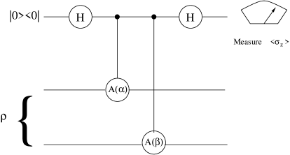
FIG. 1.: Circuit for measuring $W(\alpha_{1},\alpha_{2})$, for a composite system. The controlled operations apply the operator $2N\hat{A}(\alpha_{i})$ (which is unitary) conditioned on the state of the ancilla qbit. The phase space operators parametrically depend on the phase space point $\alpha_{i}$ and can be efficiently built as a simple sequence of displacements and reflections on each of the two subsystems. The measured polarization of the ancilla qbit is directly proportional to the Wigner function.

From the previous discussion it is clear that the above algorithm is such that by measuring the polarization of the ancillary qbit we determine the Wigner function. Indeed, this follows from the identity

$$\langle\sigma_{z}\rangle=4N^{2}{\mbox{Tr}}(\rho\hat{A}(\alpha_{1})\otimes\hat{A}(\alpha_{2}))=4N^{2}W(\alpha_{1},\alpha_{2}).$$ (66)

As phase space point operators (6) are simply a product of displacement operators (which implement addition of one, modulo $N$) and reflections (which are the square of the Fourier transform) the network of Figure 1 can be implemented efficiently (i.e., it involves a number of elementary gates that grows polynomially with $\log(N)$).

V Conclusion

In this paper we used a hybrid approach to construct a Wigner function to represent quantum states of a composite system in phase space. The function we defined has interesting features enabling us to study situations where entanglement between subsystems plays an important role. Thus, the hybrid method captures some of the most useful properties of the Wigner functions defined by Wooters [10] and Leonhardt (and others)[11, 16]. For a bipartite system this function depends upon two phase space coordinates $W(\alpha_{1},\alpha_{2})$. The phase space is a Cartesian product of the phase spaces of the subsystems, as it is the case in Wotters proposal. However, each phase space grid has $2N\times 2N$ points, as suggested by Leonhardt and others. For separable states the Wigner function is, in general, a convex sum of products of independent functions for each subsystem. Thus, this Wigner function is a natural tool to study entanglement between subsystems. In this paper we showed that basis of entangled states can be identified with non–separable slices in the phase space (the basis formed by Bell states is one such example). We also showed that $W(\alpha,\alpha^{\prime})$ is measurable by a simple scattering–like experiment where an ancillary particle successively interacts with the two subsystems.

- [1] C. H. Bennett, G. Brassard, C. Crépeau, R. Jozsa, A. Peres and W. K. Wooters, Phys. Rev. Lett. 70, 1895 (1993).
- [2] D. Bouwmeester, J-W. Pan, K. Mattle, M. Eibl, H. Weinfurter and A. Zeilinger, Nature 390 575 (1997).
- [3] ”Quantum Information and Computation”, I. Chuang and M. Nielsen (2000), Cambridge University Press.
- [4] D. Gottesman and I. Chuang, Nature 402 390 (1999).
- [5] L. Vaidman, Phys. Rev. A49, 1473 (1993).
- [6] S.L. Braunstein and H. J. Kimble, Phys. Rev. Lett. 80 869 (1999).
- [7] A. Furusawa et al, Science 282 (1998) 706.
- [8] M. Hillery, R.F. O’Connell, M.O. Scully, E. P. Wigner, Phys. Rep.106 121 (1984).
- [9] M. Koniorczyk, V. Buzek and J. Jansky, Phys. Rev. A64 (2001) 034301.
- [10] W. K. Wooters, Ann. Phys. NY 176 (1987), 1
- [11] U.Leonhardt, Phys. Rev. Lett. 74 (1995) 4101; U.Leonhardt, Pys. Rev. A 53 (1996) 2998.
- [12] J. H. Hannay, M. V. Berry, Physica 1D (1980) 267.
- [13] A. Rivas, A. M. Ozorio de Almeida, Ann.Phys. 276 (1999), 123
- [14] A. Bouzouina, S. De Bievre, Comm. Math. Phys. 178 (1996)83
- [15] P. Bianucci, C. Miquel, J. P. Paz and M. Saraceno, Discrete Wigner functions and the phase space representation of a quantum computer quant-ph/0105091.
- [16] C. Miquel, J. P. Paz and M. Saraceno, Quantum computers in phase space, (2001), submitted to PRA.
- [17] J. Schwinger, Proc. Nat. Acad, Sci.46 (1960), 570, 893.
- [18] A. Einstein, B. Podolsky and N. Rosen, Phys. Rev 47 (1935) 777.
- [19] T. J. Dunn et al., Phys. Rev. Lett. 74 (1994) 884; D. Leibfried et al., Phys. Rev. Lett. 77 (1996) 4281; see also Physics Today 51 no. 4 (1998) 22; L. Lvovsky et al., Phys. Rev. Lett. 8705 (2001) 050402.
- [20] L. G. Lutterbach and L. Davidovich, Phys. Rev. Lett. 78 (1997) 2547; Optics Express 3 (1998) 147.
- [21] G. Nogues et al, Phys. Rev. A62 (2000) 054101
- [22] C. Miquel, J.P. Paz, M. Saraceno, E. Knill, R. Laflamme, C. Negrevergne (2001), quant-ph/0109072.