Quantum computers in phase space

Abstract

We represent both the states and the evolution of a quantum computer in phase space using the discrete Wigner function. We study properties of the phase space representation of quantum algorithms: apart from analyzing important examples, such as the Fourier Transform and Grover’s search, we examine the conditions for the existence of a direct correspondence between quantum and classical evolutions in phase space. Finally, we describe how to directly measure the Wigner function in a given phase space point by means of a tomographic method that, itself, can be interpreted as a simple quantum algorithm.

2

I Introduction

Quantum mechanics can be formulated in phase space, the natural arena of classical physics. For this we can use the Wigner function [1], which is a distribution enabling us to represent quantum states and temporal evolution in the classical phase space scenario. In this paper we use the generalization of the familiar Wigner representation of quantum mechanics to the case of a system with a finite, $N$–dimensional, Hilbert space. Our main purpose is to develop and study the phase space representation of both the states and the evolution of a quantum computer (some steps in this direction were described in [2]).

One can ask if there are potential advantages in using a phase space representation for a quantum computer. The use of this approach is quite widespread in various areas of physics (such as quantum optics, see [3] for a review) and has been fruitful, for example, in analyzing issues concerning the classical limit of quantum mechanics [4, 5]. In answering the above question one should have in mind that a quantum algorithm can be simply thought of as a quantum map acting in a Hilbert space of finite dimensionality (a quantum map should be simply thought of as a unitary operator that is applied successively to a system). Therefore, any algorithm is clearly amenable to a phase space representation. Whether this representation will be useful or not will depend on properties of the algorithm. Specifically, algorithms become interesting in the large $N$ limit (i.e. when operating on many qubits). For a quantum map this is the semiclassical limit where regularities may arise in connection with its classical behavior. Unraveling these regularities, when they exist, becomes an important issue which can be naturally accomplished in a phase space representation. Therefore, having in mind these ideas, we conjecture that this representation may be useful to analyze some classes of algorithms. Moreover, the phase space approach may allow one to establish contact between the vast literature on quantum maps (dealing with their construction, the study of their semiclassical properties, etc) and that of quantum algorithms. This, in turn, may provide hints to develop new algorithms and ideas for novel physics simulations. As a first application of these ideas in this paper we examine several properties of quantum algorithms in phase space: We analyze under what circumstance it is possible to establish a direct classical analogue for a quantum algorithm (exhibiting interesting examples of this kind, such as the Fourier transform and other examples which naturally arise in studies of quantum maps). We also shown that, quite surprisingly, Grover’s search algorithm [6] can be represented in phase space and interpreted as a simple quantum map.

To define Wigner functions for discrete systems various attempts can be found in the literature. Most notably, Wooters [7] proposes a definition that has all the desired properties (see below) only when $N$ is a prime number. His phase space is an $N\times N$ grid (if $N$ is prime) and a Cartesian product of spaces corresponding to prime factors of $N$ in the general case. Our approach here follows Wooters ideas and is closely related to that of Leonhardt [8] who analyzed Wigner functions for spin systems (both in the integer and half–integer case) and discussed interesting tomographic schemes to reconstruct the quantum state from measurements of marginal distributions. Other works connected to ours are those of Hannay and Berry [9], who used discrete Wigner function in the context of studies of quantum chaos; Rivas and Ozorio [10] who define translation and reflection operators relating to the geometry of chords and centers on the phase space torus. Bouzouina and De Bievre [11] give a more abstract derivation of the same Wigner function related to geometric quantization.

The paper is organized as follows: In Section II we briefly discuss the main properties of the Wigner representation in the continuous case. In Section III we review the main features of the discrete Wigner function. This section is supposed to be self contained and to summarize known results (it also contains some original results and new explanations of old ideas). In Section IV we examine the Wigner function of quantum states, some of which are of interest for quantum computation. In Section V we review the main properties of the temporal evolution in the Wigner representation. Here we describe some general results on the nature of temporal evolution in phase space and draw important analogies between quantum algorithms and maps. We explicitly analyze Grover’s algorithm in phase space and also discuss the conditions for quantum evolution to have a direct correspondence with a classical map. In Section VI we consider the measurement of the Wigner function. We show that this can be done by means of a simple quantum computation that bears a remarkable similarity with a simulated scattering experiment. In Section VII we present our conclusions.

II Continuous Wigner functions

For a particle in one dimension, the Wigner function [1] is in one to one correspondence with the density matrix $\hat{\rho}$ and is defined as

$$W(q,p)=\int{{d\lambda}\over{2\pi\hbar}}\mbox{e}^{i\lambda p/\hbar}\,\langle q-\lambda/2|\hat{\rho}|q+\lambda/2\rangle.$$ (1)

This function is the closest one can get to a phase space distribution for a quantum mechanical system. It’s three defining properties are: (P1) $W(q,p)$ is real valued, (P2) the inner product between states $\hat{\rho}_{1}$ and $\hat{\rho}_{2}$ can be computed from the Wigner function as $\mbox{Tr}[\hat{\rho}_{1}\hat{\rho}_{2}]=2\pi\hbar\int dqdpW_{1}(q,p)W_{2}(q,p)$ and (P3) the integral along any line in phase space, defined by the equation $a_{1}q+a_{2}p=a_{3}$, is the probability density that a measurement of the observable $a_{1}\hat{Q}+q_{2}\hat{P}$ has $a_{3}$ as its result. This last property (the fact that $W(q,p)$ yields the correct marginal distribution for any quadrature) is the most restrictive one and, as Bertrand and Bertrand showed [12], together with P1–P2, uniquely determines the Wigner function.

It is convenient to write $W(q,p)$ as the expectation value of an operator, known as “phase space point operator” [7] (or Fano operators [13]). In fact, the Wigner function is

$$W(q,p)=\mbox{Tr}[\hat{\rho}\,\hat{A}(q,p)\,].$$ (2)

The operators $\hat{A}(q,p)$ depend parametrically on $q$, $p$ and can be written in terms of simetrized products of delta functions as:

$$\hat{A}(q,p) = :\delta(\hat{P}-p)\,\delta(\hat{Q}-q):$$ (3)

$$= \int{{d\lambda d\lambda^{\prime}}\over{(2\pi\hbar)^{2}}}\,\mbox{e}^{-i{\lambda\over\hbar}(\hat{P}-p)+i{{\lambda^{\prime}}\over{\hbar}}(\hat{Q}-q)}$$ (4)

$$= \int{{d\lambda d\lambda^{\prime}}\over{(2\pi\hbar)^{2}}}\,\hat{D}(\lambda,\lambda^{\prime})\,\mbox{e}^{-{i\over\hbar}(\lambda^{\prime}q-\lambda p)},$$ (5)

where we have identified the continuous translation operator $\hat{D}(\lambda,\lambda^{\prime})=\exp[-{i\over\hbar}(\lambda\hat{P}-\lambda^{\prime}\hat{Q})]$. Thus, the above expression shows that the phase space point operator is simply the double Fourier transform of the phase space displacement operator (and, therefore, $W(q,p)$ is the double Fourier transform of the expectation value of $D(\lambda,\lambda^{\prime})$). It is even more convenient to rewrite these expressions as:

$$\hat{A}(q,p)={1\over{\pi\hbar}}\hat{D}(q,p)\hat{R}\hat{D}^{\dagger}(q,p),$$ (6)

where $\hat{R}$ is the reflection (parity) operator that acts on position eigenstates as $\hat{R}|x\rangle=|-x\rangle$. This means that the Wigner function is the expectation value of a displaced reflection operator.

The proof of the three defining properties of the Wigner function (P1–P3) can be seen to follow from simple properties of the phase space point operators. The fact that $W(q,p)$ is real valued (P1) is a consequence of the hermiticity of $\hat{A}(q,p)$. Property (P2) follows from the completeness relation of $\hat{A}(q,p)$. In fact, one can show that these operators satisfy the relation

$$\mbox{Tr}[\hat{A}(q,p)\hat{A}(q^{\prime},p^{\prime})]={1\over{2\pi\hbar}}\delta(q-q^{\prime})\delta(p-p^{\prime}).$$ (7)

As a consequence of this, one can invert (2) and express the density matrix as a linear combination of the phase space point operators. The Wigner functions determines the coefficients of such expansion: $\hat{\rho}=2\pi\hbar\int dqdpW(q,p)\hat{A}(q,p)$. From this, the validity of the inner product rule can be easily demonstrated. The last property (P3) can be seen to be valid by observing that integrating $\hat{A}(q,p)$ along a line in phase space one always gets a projection operator. Thus,

$$\int dqdp\,\delta(a_{1}q+a_{2}p-a_{3})\hat{A}(q,p)=|a_{3}\rangle\langle a_{3}|,$$ (8)

where $|a_{3}\rangle$ is an eigenstate of the operator $a_{1}\hat{Q}+a_{2}\hat{P}$ with eigenvalue $a_{3}$. This identity can be shown by first writing the delta function as the integral of an exponential and then performing the phase space integration. We omit the proof here because we will present the corresponding one for the discrete case, which is done following very similar lines.

III Discrete Wigner Functions

A Preliminarities: discrete phase space

We will consider here a quantum system with an $N$ dimensional Hilbert space (the case of a quantum computer is a specific example we will always have in mind but the formalism can be applied in other cases). In the Hilbert space we can introduce a basis $B_{x}=\{|n\rangle,n=0,\ldots,N-1\}$ which we arbitrarily interpret as our discretized position basis (with periodic boundary conditions: $|n+N\rangle=|n\rangle$). Clearly, the notion of a position observable may not have a direct physical interpretation in a discrete system but is a necessary ingredient if one wants to build a phase space representation. In the case of a quantum computer this basis can be, for example, the computational basis. Given the position basis $B_{x}$, there is a natural way to introduce the conjugate momentum basis $B_{p}=\{|k\rangle,k=0,\ldots,N-1\}$ by means of the discrete Fourier transform. Thus, the states of $B_{p}$ can be obtained from those of $B_{x}$ as

$$|k\rangle={1\over\sqrt{N}}\sum_{n}\exp(i2\pi nk/N)|n\rangle.$$ (9)

Therefore, as in the continuous case, position and momentum are related by the Fourier transform. It is also important to recognize that the dimensionality of the Hilbert space of the system is related to an effective Planck constant. In fact, phase space should have a finite area (which we consider equal to one, in the appropriate units). In this area we should be able to accommodate $N$ orthogonal states. If each of this states occupies a phase space area which is equal to $2\pi\hbar$, we see that:

$$N=1/2\pi\hbar.$$ (10)

In other words, $N$ plays the role of the inverse of the Planck constant (and the large $N$ limit is, in some way, the semiclassical limit).

Once we have position and momentum basis we can construct the displacement operators in position and momentum. Obviously, in this case it does not make sense to talk about infinitesimal translations. However, for discrete systems we can define finite translation operators $\hat{U}$ and $\hat{V}$, which respectively generate finite translations in position and momentum [14]. The translation operator $\hat{U}$ generates cyclic shifts in the position basis and is diagonal in momentum basis:

$$\hat{U}^{m}|n\rangle=|n+m\rangle,\ \hat{U}^{m}|k\rangle=\exp(-2\pi imk/N)|k\rangle,$$ (11)

(note that all additions inside kets are to be interpreted mod $N$). Similarly, the operator $\hat{V}$ is a shift in the momentum basis and is diagonal in position:

$$\hat{V}^{m}|k\rangle=|k+m\rangle,\ \hat{V}^{m}|n\rangle=\exp(i2\pi mn/N)|n\rangle$$ (12)

It is important to notice that the translation operators $\hat{U}$ and $\hat{V}$ have commutation relations that directly generalize the ones corresponding to finite position and momentum translations in the continuous case. In fact, one can directly show the following identity:

$$\hat{V}^{p}\hat{U}^{q}=\hat{U}^{q}\hat{V}^{p}\exp(i2\pi pq/N).$$ (13)

With these tools at hand we can introduce the discrete analog to the continuous phase space translation operator $\hat{D}(q,p)=\exp[-{i\over\hbar}(q\hat{P}-p\hat{Q})]$. To do this we can first rewrite the phase space displacement as $\hat{D}(q,p)=\exp(-iq\hat{P}/\hbar)\,\exp(ip\hat{Q}/\hbar)\,\exp(ipq/2\hbar)$ (an expression obtained by using the well known formula $\mbox{e}^{\hat{A}+\hat{B}}=\mbox{e}^{-[\hat{A},\hat{B}]/2}\,\mbox{e}^{\hat{A}}\mbox{e}^{\hat{B}}$ and the canonical commutation relation between $\hat{Q}$ and $\hat{P}$). Therefore, by identifying the corresponding displacement operators, the discrete analogue of the phase space translation operator is:

$$\hat{T}(q,p)\equiv\hat{U}^{q}\hat{V}^{p}\exp(i\pi qp/N).$$ (14)

These operators obey the simple composition rule

$$\hat{T}(q_{1},p_{1})\hat{T}(q_{2},p_{2})=\hat{T}(q_{1}+q_{2},p_{1}+p_{2}){\rm e}^{i\pi(p_{1}q_{2}-q_{1}p_{2})/N},$$ (15)

where the phase appearing in the left hand side has a simple geometrical interpretation as the area of a triangle (see below). From the above definitions it is also simple to show that the phase space translation operators are such that

$$\hat{T}^{\dagger}(q,p) = \hat{T}(2N-q,2N-p)$$ (16)

$$= \hat{T}(N-q,N-p)\,(-1)^{N+p+q}.$$ (17)

Finally, it is worth mentioning the fact that the composition rule can be used to show that

$$\hat{T}(\lambda q,\lambda p)=\hat{T}^{\lambda}(q,p)$$ (18)

for any integer $\lambda$, which is a very natural result. It may be tempting to define position and momentum operators also in the discrete case. In fact, we could attempt doing that by writing $\hat{U}$ and $\hat{V}$ as the exponentials of two operators $\hat{Q}$ and $\hat{P}$ defined to be diagonal in $B_{x}$ and $B_{p}$ respectively: $\hat{U}=\exp(-i2\pi\hat{P}/N)$ and $\hat{V}=\exp(i2\pi\hat{Q}/N)$, with $\hat{Q}\equiv\sum_{n}n|n\rangle\langle n|$ and $\hat{P}\equiv\sum_{k}k|k\rangle\langle k|$. However, it turns out that these operators are not canonically conjugate since their commutator is not proportional to the identity as is the continuous case (actually, it is well known that for finite dimensional spaces it is impossible to find two operators whose commutator is proportional to the identity). So, even though finite shifts in the discrete case have the same properties than their continuous counterparts, this is not true for the position and momentum operators.

It will also be useful to define a reflection (or parity) operator $\hat{R}$ as the one acting on states in the position (and momentum) basis as $\hat{R}|n\rangle\equiv|-n\rangle$ (again, the operation is to be understood mod $N$). It is simple to show that the parity operator obeys simple relations with the shifts $\hat{U}$ and $\hat{V}$:

$$\hat{U}\hat{R}=\hat{R}\hat{U}^{-1},\ \hat{V}\hat{R}=\hat{R}\hat{V}^{-1}.$$ (19)

It is important to recognize that the reflection operator is directly related to the Fourier transform. In fact, if we denote the operator implementing the discrete Fourier transform as $U_{FT}$ (i.e., the operator whose matrix elements in the $B_{x}$ basis are $\langle n^{\prime}|U_{FT}|n\rangle=\exp(i2\pi nn^{\prime}/N)$), then the reflection operator is simply the square of the Fourier transform:

$$\hat{R}=U_{FT}^{2}.$$ (20)

Before ending this section it is worth mentioning other possibilities for the phase space description of finite quantum mechanics. The use of the discrete Fourier transform to relate position and momentum implies the imposition of periodic boundary conditions on both these variables, thus imposing the geometry of a torus on the phase space. This is by no means mandatory, as the well known example of the angular momentum sphere –spanned by states $|j,m\rangle,m=-j,...j$– illustrates. However, the ubiquitous appearance of the DFT in quantum algorithms somehow favors the choice of the torus as the preferred geometry. It is also possible to slightly extend the scope of the present approach by imposing quasi-periodic boundary conditions, as is done in solid state chain models or in the treatment of the quantum Hall effect. This generalization can be easily incorporated into the description of quantum algorithms [15]

B Discrete Wigner functions and phase space point operators

To define a discrete Wigner function the most convenient strategy is to find the correct generalization of the phase space point operators $\hat{A}(q,p)$. Thus, we need to find a basis set of the space of hermitian operators (note that, as the Hilbert space is $N$ dimensional such a basis has $N^{2}$ independent operators). We should do this in such a way that the resulting Wigner function gives the correct marginal distributions. However, generalization from the continuous to the discrete case has to be done with some caution. In fact, it is instructive to see how naive attempts to generalize expressions like (5) or (6) fail. In fact, generalizing equation (5) to the discrete case would lead us to define

$$\hat{\cal A}(q,p)={1\over N^{2}}\sum_{m,k=0}^{N-1}\hat{T}(m,k)\exp{\{-i2\pi{(kq-mp)\over N}\}}.$$ (21)

Unfortunately, this expression for $\hat{\cal A}(q,p)$ turns out to be non–hermitian. This can be seen by taking the hermitian conjugate of the above equation and using the fact that the Hermitian conjugate of the phase space translation operator, as shown in (17), is such that $\hat{T}^{\dagger}(q,p)\neq\hat{T}(N-q,N-p)$. Therefore, the above is not a good definition for the discrete phase space point operators.

Another naive attempt to define discrete phase space operators is to generalize equation (6) which tells us that in the continuous case the operator $\hat{A}(q,p)$ is a displaced reflection. Thus, by writing

$$\hat{A}(q,p)={1\over{\pi\hbar}}\hat{D}(q,p)\hat{R}\hat{D}^{\dagger}(q,p)\rightarrow{1\over N/2}\hat{T}(q,p)\hat{R}\hat{T}^{\dagger}(q,p),$$ (22)

one defines an operator that is hermitian by construction. However, in this case the problem is that the number of operators one defines in this way is not enough to build a complete set. In fact, if one uses the definition of $\hat{T}(q,p)$ given in (14) and then the commutation relations between $\hat{U}$, $\hat{V}$ and $\hat{R}$ one finds:

$$\hat{A}(q,p)={1\over N}\,\hat{U}^{2q}\hat{R}\hat{V}^{-2p}\exp(4\pi i\,pq/N).$$ (23)

As $\hat{U}$ and $\hat{V}$ are cyclic operators with period $N$, it is easy to see that if both $q$ and $p$ take values between $0$ and $N$ the above expression only gives $N^{2}/4$ independent operators. In fact, it is clear that the above equation implies that $\hat{A}(q+N/2,p)=\hat{A}(q,p)$ and likewise with $p$ so we only have $N/2\times N/2$ independent operators.

Remarkably, the solution to the problems arising with the two above naive definitions is obviously the same: We should define, as it is done in the literature [9, 11] the phase space point operators on a phase space grid of $2N\times 2N$ points. This can be done simply replacing $N\rightarrow 2N$ in equation (21) or by taking half integer values for $q$ and $p$ in (23). The two definitions turn out to be equivalent. Therefore, the correct discrete phase space point operators are

$$\hat{A}(\alpha) = {1\over(2N)^{2}}\sum_{\lambda,\lambda^{\prime}=0}^{2N-1}\hat{T}(\lambda,\lambda^{\prime})\exp{\{-i2\pi{(\lambda^{\prime}q-\lambda p)\over 2N}\}}$$ (24)

$$= {1\over{2N}}\hat{U}^{q}\hat{R}\hat{V}^{-p}\exp(i\pi pq/N)$$ (25)

where $\alpha=(q,p)$ denotes a point in the phase space grid with $q$ and $p$ taking values between $0$ and $2N-1$.

It is worth noticing that, as we have just defined phase space point operators on a lattice with $2N\times 2N$ points, we have a total of $4N^{2}$ such operators. However, it should be clear that these operators are not all independent. It is easy to verify that there are only $N^{2}$ independent phase space point operators since it can be proved that:

$$\hat{A}(q+\sigma_{q}N,p+\sigma_{p}N)=\hat{A}(q,p)\,(-1)^{\sigma_{p}q+\sigma_{q}p+\sigma_{q}\sigma_{p}N},$$ (26)

for $\sigma_{q},\sigma_{p}=0,1$. Therefore, it is clear that the $N^{2}$ phase space point operators corresponding to the first $N\times N$ subgrid of the phase space determine the rest. For the rest of the paper we will denote the first $N\times N$ subgrid as the set $G_{N}$ (i.e., $G_{N}=\{\alpha=(q,p);0\leq q,p\leq N-1\}$). The set $G_{2N}$ will denote the full $2N\times 2N$ grid.

Before showing explicitly that the above operators enable us to define a Wigner function with all the desired properties, it is worth pointing out some useful facts about $\hat{A}(\alpha)$. In particular, it is convenient to realize that these operators are closely related to the phase space translation operators. In fact, one can show that by successive application of two phase space operators one always gets a translation (this is also true in the continuous case) since

$$\hat{A}(\alpha)\hat{A}(\alpha^{\prime})=\hat{T}(\alpha-\alpha^{\prime})\,{{\mbox{e}}^{i{\pi\over N}(q_{\alpha}p_{\alpha^{\prime}}-q_{\alpha^{\prime}}p_{\alpha})}\over{4N^{2}}}$$ (27)

Moreover, it is also useful to express the translation operator in terms of the $\hat{A}(\alpha)$ operators by simply inverting the defition (24) and writing

$$\tilde{T}(n,k)=\sum_{q,p=0}^{2N-1}\,\hat{A}(q,p)\ \exp(-i{2\pi\over{2N}}(np-kq)),$$ (28)

a property that is also valid in the continuous case.

From the above properties it is possible to show that $\hat{A}(\alpha)$ are a complete set when $\alpha$ takes values in the first $N\times N$ subgrid $G_{N}$. Thus, taking the trace of (27) one gets:

$$\mbox{Tr}[\hat{A}(\alpha)\hat{A}(\alpha^{\prime})]={1\over{4N}}\,\delta_{N}(q^{\prime}-q)\delta_{N}(p^{\prime}-p)$$ (29)

where both $\alpha$ and $\alpha^{\prime}$ are in the grid $G_{N}$ and $\delta_{N}(q)\equiv{1\over N}\sum_{n=0}^{N-1}\mbox{e}^{2\pi iq/N}$ is the periodic delta function (which is zero unless $q=0\ \mbox{mod}\ N$).

Therefore, according to all the previous arguments, the discrete Wigner function is defined as

$$W(\alpha)=\mbox{Tr}(\hat{A}(\alpha)\hat{\rho})$$ (30)

where $\alpha\in G_{2N}$. Clearly, these $4N^{2}$ values are not all independent since the Wigner function obeys the same relation than the phase space point operators:

$$\hat{W}(q+\sigma_{q}N,p+\sigma_{p}N)=\hat{W}(q,p)\,(-1)^{\sigma_{p}q+\sigma_{q}p+\sigma_{q}\sigma_{p}N}$$ (31)

As the operators $\hat{A}(\alpha)$ are a complete set one can expand the density matrix as a linear combination of such operators. It is clear that the Wigner function $W(\alpha)$ are nothing but the coefficients of such expansion. Thus, one can show that

$$\hat{\rho} = 4N\,\sum_{\alpha\in G_{N}}W(\alpha)\hat{A}(\alpha)$$ (32)

$$= N\,\sum_{\tilde{\alpha}\in G_{2N}}W(\tilde{\alpha})\hat{A}(\tilde{\alpha}).$$ (33)

The last expression can be obtained from (32) by noticing that the contribution arising from the four $N\times N$ subgrids are identical.

Now it is simple to show that the Wigner function defined above obeys the three defining properties (P1–P3). The first one is a consequence of the fact that the operators $\hat{A}(\alpha)$ are hermitian by construction. The second property (P2) is a consequence of the completeness of the set $\hat{A}(\alpha)$ which enables one to show that

$$\mbox{Tr}[\rho_{1}\rho_{2}]=N\sum_{\alpha\in G_{2N}}W_{1}(\alpha)W_{2}(\alpha)$$ (34)

Finally, the third property (P3) is more subtle and deserves to be studied with some detail. The crucial point is to show that if we add the operators $\hat{A}(q,p)$ over all phase space points lying on a line $L$ we always obtain a projection operator (this guarantees that adding the value of the Wigner function over all points in a line gives always a positive number, which can be interpreted as a probability). Before showing this, we should clearly define what do we mean by a line $L(n_{1},n_{2},n_{3})$ on our phase space grid. We will use the following definitions: A line $L$ is a set of points of the grid defined as $L=L(n_{1},n_{2},n_{3})=\{(q,p)\in G_{2N},\ \mbox{such that}\ n_{1}p-n_{2}q=n_{3}$, with $0\leq n_{i}\leq 2N-1\}$. Below, we will discuss some more details about the structure of lines on a grid $G_{2N}$. Here, we only need to point out that one can also define a notion of parallelism between lines: two lines parametrized by the same set of integers $n_{1}$ and $n_{2}$ are parallel to each other (in Figure (1) we show some examples of lines on a grid).

So, let us show that by adding phase space point operators on a line one always gets projection operators. We are interested in looking at the operator $\hat{A}_{L}$ defined as

$$\hat{A}_{L}=\sum_{(q,p)\in L}\hat{A}(q,p).$$ (35)

It is clear that this operator can be rewritten as

$$A_{L} = \sum_{q,p=0}^{2N-1}\ \hat{A}(q,p)\ \delta_{2N}(n_{1}p-n_{2}q-n_{3})$$ (36)

$$= {1\over 2N}\sum_{\lambda=0}^{2N-1}\ \sum_{q,p=0}^{2N-1}\ \hat{A}(q,p)\ \mbox{e}^{-i{2\pi\over{2N}}\lambda(n_{1}p-n_{2}q-n_{3})}$$ (37)

$$= {1\over 2N}\ \sum_{\lambda=0}^{2N-1}\hat{T}^{\lambda}(n_{1},n_{2})\ \mbox{e}^{i{2\pi\over{2N}}n_{3}\lambda}$$ (38)

where to perform the sum over the phase space grid we used the fact that the Fourier transform of $\hat{A}(\alpha)$ is given in (28). Now, as $\hat{T}(n_{1},n_{2})$ is unitary, it has $N$ eigenvectors $|\phi_{j}\rangle$ with eigenvalues $\exp(-i2\pi\phi_{j}/N)$. Moreover, this operator is cyclic and satisfies $\hat{T}^{N}={\mathbb{I}}$. Therefore, as its eigenvalues are $N$th roots of unity, $\phi_{j}$ must be integers. Then, we can rewrite equation (38) as:

$$\hat{A}_{L} = {1\over 2N}\sum_{\lambda=0}^{2N-1}\ \sum_{j=0}^{N}\mbox{e}^{-i{{2\pi}\over{2N}}(2\phi_{j}-n_{3})\lambda}\ |\phi_{j}\rangle\langle\phi_{j}|$$ (39)

$$= \ \sum_{j=0}^{N}\delta_{2N}(2\phi_{j}-n_{3})\ |\phi_{j}\rangle\langle\phi_{j}|.$$ (40)

Therefore, it is clear that $\hat{A}_{L}$ is a projection operator onto a subspace generated by a subset of the eigenvectors of the translation operator $\hat{T}(n_{1},n_{2})$. The dimensionality $d$ of this subspace is equal to the trace of $\hat{A}_{L}$. To calculate it, we just have to notice that in general

$$\mbox{Tr}[\hat{A}(q,p)]={1\over{2N}}\sum_{q^{\prime}=0}^{N-1}\delta_{N}(q-2q^{\prime})\ \mbox{e}^{i\pi(q-2q^{\prime})p/N}$$ (41)

This last equation is easy to evaluate but the result depends on the parity of $N$. Thus, if $N$ is even then $\mbox{Tr}(\hat{A}(q,p))=1/N$ if both $q$ and $p$ are even and it is zero otherwise. On the other hand for odd values of $N$, one has that $\mbox{Tr}(\hat{A}(q,p))=1/2N$ for all values of $q$ and $p$ except when they are both odd where it has the opposite sign (i.e., it is equal to $-1/2N$). In the rest of the paper we will concentrate on analyzing the case of even $N$ which is somewhat more relevant for a quantum computer (that has at least one qubit and therefore a Hilbert space which is even dimensional). Using the above result for the trace of $\hat{A}(\alpha)$ one can see that the dimensionality of the projector $\hat{A}_{L}$ is simply given by $1/N$ times the number of points that belong to the line $L$ which have even $q$ and even $p$ coordinates. An immediate consequence of this is that if $n_{3}$ is odd then $d=0$ (since the sum of two even numbers can never be odd). Finally we can write an explicit formula for $d$ in the case of even $N$:

$$d={1\over 2}\,\sum_{\lambda=0}^{N-1}\ \delta_{N}(\lambda n_{1})\delta_{N}(\lambda n_{2})\mbox{e}^{i{2\pi m\lambda\over 2N}}\,(1+(-1)^{n_{3}})$$ (42)

Let us illustrate the above result applying it to the simplest example: For a line $L_{q}$ defined as $q=n_{3}$ (i.e., $n_{1}=1$, $n_{2}=0$), the Wigner function summed over all points in $L_{q}$ is $\sum_{(q,p)\in L_{q}}W(q,p)=\sum_{p}W(n_{3},p)=\langle n_{3}/2|\hat{\rho}|n_{3}/2\rangle$ if $n_{3}$ is even (and zero otherwise). Analogously, considering horizontal lines ($L_{p}$ defined as $p=n^{\prime}_{3}$) we get $\sum_{(q,p)\in L_{p}}W(q,p)=\sum_{q}W(q,n^{\prime}_{3})=\langle n^{\prime}_{3}/2|\hat{\rho}|n^{\prime}_{3}/2\rangle$ if $n^{\prime}_{3}$ is even (and zero otherwise). These are just two examples a general result: this Wigner function always generates the correct marginal distributions (this, as in the continuous case, is the defining feature of $W(q,p)$).

As a final point in this section where we reviewed some known (and other not so well known) results on discrete Wigner functions we think it is convenient to mention some simple properties of the phase space grid $G_{2N}$. Most of the ideas we are using were introduced by Wootters [7]. As mentioned above we can simply define lines $L(n_{1},n_{2},n_{3})$ and introduce a notion of parallelism in the grid $G_{2N}$. A foliation of the grid with a family of parallel lines is obtained by fixing $n_{1}$ and $n_{2}$ and varying $n_{3}$ (in general, it is evident that two lines are parallel if the ratio $n_{1}/n_{2}$ is the same). If $N$ is a prime number then in the grid $G_{N}$ (which has $N\times N$ points) there are exactly $N(N+1)$ distinct lines which can be grouped into $N+1$ sets of parallel lines (these are $N+1$ different foliations of the grid). If $N$ is not prime or, as it is the case we are interested in, in the grid $G_{2N}$ this result is no longer true. For example, it is very clear that the equation $n_{1}q-n_{2}p=n_{3}$ (mod $2N$) has no solutions for odd values of $n_{3}$ and even values of $n_{1}$ and $n_{2}$. So, it is not generally true that our lines have always $2N$ points: As shown above sometimes they can have no points at all and in some cases one can construct lines with a number of points that is a multiple of $2N$. This is the case if $n_{1}$ and $n_{2}$ have common prime factors with $N$. For example in the case $2N=8$, each line with $n_{1}=n_{2}=1$ have $8$ points, but lines with $n_{1}=n_{2}=2$ have no points if $n_{3}$ is odd or $16$ points each when $n_{3}$ is even. In any case, the simplest way to represent the lines in the phase space is by noticing that, as the topology of the lattice is that of a torus (due to the cyclic boundary conditions) lines wrap around the torus. The number of points in the line is related to the number of times it wraps around before it closes onto itself. Figure 1 shows an example of two sets of lines on the grid $G_{2N}$ for the case of $N=4$.

FIG. 1.: Left: lines satisfying the equation $p+q=n_{3}$ (mod $8$) for values $n_{3}=0,2$. Each line has 8 points and there are a total of 8 distinct lines. Right: two of the four possible lines satisfying $2p+2q=n_{3}$ with $n_{3}=0,2$. In both plots horizontal (vertical) axis corresponds to position (momentum) basis.

Let us summarize the results presented in this Section: We defined a Wigner function for systems with a finite dimensional Hilbert space (of arbitrary dimension $N$). The Wigner function is defined as the expectation value of the phase space operator $\hat{A}(\alpha)$ given in (25). This definition is such that $W(\alpha)$ is real, it can be used to compute inner products between states and it gives all the correct marginal distributions when added over any line in the phase space, which is a grid $G_{2N}$ with $2N\times 2N$ points. The size of the phase space grid is important to obtain a Wigner function with all the desired properties. The values of $W(\alpha)$ on the subgrid $G_{N}$ are enough to reconstruct the rest of the phase space (since the set $\hat{A}(\alpha)$ is complete when $\alpha$ belong to the grid $G_{N}$). However, the redundancy introduced by the doubling of the number of sites in $q$ and $p$ is essential when one imposes the condition that all the marginal distributions should be obtained from the Wigner function. In the rest of the paper we will concentrate on applying this Wigner function to study the states and the evolution of a typical quantum computer.

IV Wigner Functions of quantum states

To compute the Wigner function of any quantum state it is convenient to use equation (25) for $\hat{A}(q,p)$ and write:

$$W(q,p)\equiv{1\over{2{N}}}\sum_{n=0}^{N-1}\langle q-n|\hat{\rho}|n\rangle\mbox{e}^{i{2\pi\over N}n(p-q/2)}.$$ (43)

Moreover, it is worth remembering that one only needs to compute $N^{2}$ independent values (restricting to $\alpha=(q,p)\in G_{N}$) and from them one can reconstruct the remaining $3N^{2}$ ones by using (31). Before showing the specific form of the Wigner function of some states it is worth mentioning some general features of the Wigner function of pure states. In fact, if the quantum state is pure then $\hat{\rho}$ is a projection operator. Then, expanding $\hat{\rho}$ in terms of the phase space operators as in (33) and imposing the condition $\hat{\rho}^{2}=\hat{\rho}$ one gets

$$W(\alpha)=4N^{2}\sum_{\beta\gamma\in G_{N}}\Gamma(\alpha,\beta,\gamma)W(\beta)W(\gamma).$$ (44)

where the function $\Gamma(\alpha,\beta,\gamma)$, that depends on three phase space points (i.e, on a triangle) is

$$\Gamma(\alpha,\beta,\gamma) = \mbox{Tr}(\hat{A}(\alpha)\hat{A}(\beta)\hat{A}(\gamma))$$ (45)

$$= {1\over 4N^{3}}\mbox{e}^{i{2\pi\over N}{\sl S}(\alpha,\beta\gamma)}$$ (46)

if either two or three of the points $(\alpha,\beta,\gamma)$ have even $q$ and even $p$ coordinates. Otherwise $\Gamma(\alpha,\beta,\gamma)=0$. In the above expression, which is valid for even values of $N$, ${\sl S}(\alpha,\beta,\gamma)$ is the area of the triangle formed by the three phase space points (measured in units of the elementary triangle formed when the three points are one site apart). A similar expression is obtained by Wooters [7]. The three point function $\Gamma(\alpha,\beta,\gamma)$ has then a simple geometric meaning and will play an interesting role in determining the properties of the temporal evolution (as Unitary evolution preserves pure states, it will be represented by a linear map in phase space that leaves $\Gamma$ invariant, as shown see below).

A Position and momentum eigenstates, and their superpositions

Here, we first evaluate the Wigner function of a position eigenstate (a computational state of the quantum computer) $\hat{\rho}_{q_{0}}=|q_{0}\rangle\langle q_{0}|$. It is straightforward to obtain a closed expression for $W(q,p)$:

$$W_{q_{0}}(q,p) = {1\over{2N}}\langle q_{0}|\hat{U}^{q}\hat{R}\hat{V}^{-p}|q_{0}\rangle\mbox{e}^{i\pi pq/N}$$ (47)

$$= {1\over{2N}}\delta_{N}(q-2q_{0})\ (-1)^{p(q-2q_{0})_{N}}$$ (48)

where $z_{N}$ denotes $z$ modulo $N$. This function is zero only on two vertical strips located at $q=2q_{0}$ modulo $N$. When $q=2q_{0}$, $W(q,p)$ takes the constant value $1/2N$ while for $q=2q_{0}\pm N$ it is $1/2N$ for even values of $p$ and $-1/2N$ for odd values. These oscillations are typical of interference fringes and can be interpreted as arising from interference between the $q=2q_{0}$ strip and a mirror image formed at a distance $2N$ from $2q_{0}$, which is induced by the periodic boundary conditions. The fact the the Wigner function becomes negative in this interference strip is essential to recover the correct marginal distributions. Adding the values of $W(q,p)$ along a vertical line gives the probability of measuring $q/2$ which should be $1$ for $q=2q_{0}$ and zero otherwise. A very similar calculation can be done for a momentum eigenstate $\hat{\rho}=|k_{0}\rangle\langle k_{0}|$. The result is very similar except that now the strips are horizontal.

It is interesting to analyze also the Wigner function of a state which is a linear superposition $|\psi\rangle=\left(|q_{0}\rangle+\mbox{e}^{-i\phi}|q_{1}\rangle\right)/\sqrt{2}$. Again one can simply get a closed expression for $W(q,p)$ which is

$$W(q,p)={1\over 2}\left[W_{q_{0}}(q,p)+W_{q_{1}}(q,p)+\Delta W_{q_{0},q_{1}}(q,p)\right]$$

where the interference term is

$$\Delta W_{q_{0},q_{1}}(q,p)\equiv{1\over N}\,\delta_{N}(\tilde{q})\,(-1)^{\tilde{q}p}\,\cos\left({{2\pi}\over\lambda}p+\phi\right),$$

with $\tilde{q}=q_{0}+q_{1}-q$ and $\lambda\equiv 2N/(q_{0}-q_{1})$. Thus, this Wigner function has two direct terms which simply correspond to the two computational states and an interference term which is peaked on the vertical strips located at the midpoint $q=q_{0}+q_{1}\ \mbox{mod}\ N$. On this strip the Wigner function oscillates with a wavelength that is inversely proportional to the separation between the main fringes. This oscillatory pattern has its corresponding mirror image and the interference between them produce some more oscillations. In figure 2 we show the Wigner function for a state and a superposition of two such computational states. The plot is much more eloquent than any equation and shows both the presence of the main peaks, its mirror images and (in the case of a superposition state) the interference fringes.

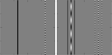
FIG. 2.: Wigner function of a position eigenstate (left) and a linear superposition of two position eigenstates (right). Horizontal (vertical) axis correspond to position (momentum) basis. For the computational state $|q_{0}\rangle$, the Wigner function is positive (black) on a vertical strip located at $q=2q_{0}$ and it has negative (white) values on another vertical strip located at $q=2q_{0}\pm N$. For a superposition of two computational states (right), the Wigner function also oscillates on the strip located at $q=q_{0}+q_{1}$ with a wavelength that depends upon the distance between the two interfering states.

B Other quantum states

The Wigner function can be computed in closed form for some other interesting states. In figure 3 we display such function for the completely mixed state (that, as we mentioned above, is nonzero only when both $q$ and $p$ are even). We also show the Wigner function for a pure state constructed as a Gaussian superposition of computational states (with periodic boundary conditions, i.e. a sum of a Gaussian state centered about a phase space point and all its infinite mirror images). The Gaussian wavepacket has a Wigner function with a positive Gaussian peak and shows three other Gaussian peaks that are modulated by interference fringes. They correspond to the interference between the main peak and its mirror images (notice the different orientation of these fringes).

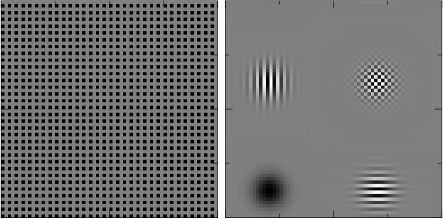
FIG. 3.: Left: Wigner function for the completely mixed state. It is positive (black) only in the phase space points with even values of $q$ and $p$ being zero (grey) elsewhere. Right: Wigner function for a periodic Gaussian wavepacket. This function has a positive (black) peak and three regions where it displays oscillatory behavior. These regions can be understood as being originated from the interference between the positive Gaussian peak and its mirror images created by the periodic boundary conditions. Horizontal (vertical) axis correspond to position (momentum) basis.

V Temporal evolution in phase space

Temporal evolution of a quantum system can also be represented in phase space. If $U$ is the unitary evolution operator that takes the state of the system from time $t$ to time $t+1$, the density matrix evolves as

$$\rho(t+1)=U\rho(t)U^{\dagger}.$$ (49)

Using this, it is simple to show that the Wigner function evolves as

$$W(\alpha,t+1)=\sum_{\beta\in G_{2N}}Z_{\alpha\beta}W(\beta,t).$$ (50)

where the matrix $Z_{\alpha\beta}$ is defined as

$$Z_{\alpha\beta}=N\quad Tr(\hat{A}(\alpha)U\hat{A}(\beta)U^{\dagger}).$$ (51)

Therefore, temporal evolution in phase space is represented by a simple linear transformation (which is, of course, an immediate consequence of linearity of Schrödinger equation). Unitarity imposes some constraints on the matrix $Z_{\alpha\beta}$: As purity of states is preserved, temporal evolution must preserve the structure of the constraint equation (44). Therefore, the matrix must leave invariant the three point function $\Gamma(\alpha,\beta,\gamma)$, i.e.

$$\Gamma(\alpha^{\prime},\beta^{\prime},\gamma^{\prime})=\sum_{\alpha\beta\gamma}Z_{\alpha^{\prime}\alpha}Z_{\beta^{\prime}\beta}Z_{\gamma^{\prime}\gamma}\Gamma(\alpha,\beta,\gamma).$$ (52)

The real matrix $Z_{\alpha\beta}$ contains all the information about the nature of temporal evolution. In general, this matrix connects a point $\alpha$ with many other points $\beta$. Therefore, temporal evolution will be generally nonlocal in phase space. This is a unique quantum mechanical feature: In fact, classical systems evolve in phase space following a flow of classical trajectories. In such case, the value of the classical distribution function $W(\alpha,t+1)$ is equal to the value $W(\beta,t)$ for some point $\beta$ which is a well defined function of $\alpha$ and $t$. One may ask what kind of Unitary operators generate a local dynamical evolution in phase space. Below, we will give examples of this type.

A Phase space translations

It is simple to show that if we consider the unitary evolution to be the phase space translation operator $\hat{T}(\sigma)=\hat{T}(q,p)$ then temporal evolution is local in phase space. Moreover, quantum and classical evolution are identical in this case since the value of the Wigner function is rigidly translated in phase space:

$$U=\hat{T}(\sigma)\iff W(\alpha,t+1)=W(\alpha-2\sigma,t).$$ (53)

Notice that the factor of $2$ in the above equation is simply a consequence of the fact that we are working in a phase space grid of $2N\times 2N$. Another example of a local evolution is the one associated with the phase space operators $\hat{A}(\alpha)$ themselves. In such case the resulting evolution is not just a translation but a translation combined with a reflection:

$$U=\hat{A}(\sigma)\iff W(\alpha,t+1)=W(2\sigma-\alpha,t).$$ (54)

The above are two simple examples of families of unitary operators with corresponding local phase space representations. As we will see below, the family of operators with a direct correspondence between quantum and classical evolution has other interesting members.

B Fourier transform

The discrete Fourier transform is a unitary operator that is widely used in quantum algorithms [6]. As position and momentum basis are related by this operator one expects that it should have a rather simple phase space representation. In fact, this is indeed the case: One can easily show that the Fourier transform is represented as a rotation in $90$ degrees:

$$U=U_{FT}\iff W(q,p,t+1)=W(-p,q,t).$$ (55)

where $-p$ is the additive inverse mod$(N)$. Thus, the Fourier transform is also represented by a local operation in phase space (and, in this sense it is a completely “classical” operation, acting independently on each of the $N\times N$ subgrid). For example, by applying the Fourier transform to the quantum states whose Wigner functions are shown in Figure 2 (a computational state and a superposition of two such states) one obtains the resulting Wigner function by rotating the above figure by $90$ degrees (i.e., one gets a momentum eigenstate or a superposition of two such states where the vertical pattern in Figure 2 is mapped into the same horizontal pattern). It is clear that by applying the Fourier transform twice one gets a rotation by $180$ degrees. This is nothing but a reflection, which is what equation (20) tells us.

C Quadratic (cat) maps propagate classically

The above operators (rigid translations, reflections and the Fourier transform) are just some examples of unitary operators which generate a classical evolution in phase space. A more general family with such property will be discussed here. This family is formed by the quantization of classical dynamical systems with a quadratic Hamiltonian and a finite phase space with periodic boundary conditions (as the phase space is a torus, the classical transformations are the linear automorphisms of the torus [16]). We will briefly present these unitary operators here and show that classical and quantum evolution coincides (a fact that has been shown before, using different techniques, by Hannay and Berry [9]). Consider the following two-parameter family of operators (it is possible to consider a slightly more general case, with one more parameter, but to simplify the presentation we restrict to this simpler case [15]).

$$U_{cat}={\cal V}_{b}{\cal T}{\cal V}_{a}.$$ (56)

The operators ${\cal V}_{a}$ and ${\cal T}$ are respectively diagonal in the position and momentum basis and satisfy

$${\cal V}_{j}|n\rangle = \exp(-i2\pi n^{2}(1-j)/2N)|n\rangle$$ (57)

$${\cal T}|k\rangle = \exp(-i2\pi k^{2}/2N)|k\rangle$$ (58)

where $j$ is an integer. The operator $U_{cat}$ can be simply thought of as the evolution operator of a kicked system with a Hamiltonian in which kinetic and momentum terms are turned on and off alternatively. The parameters $a$ and $b$ are integers that measure the strength of the potential kicks. It is straightforward to find out what is the classical system to which the above operator corresponds: One way to do this is to take the matrix elements of (56) in the computational basis and show that

$$\langle n^{\prime}|U_{cat}|n\rangle=K\exp(i2\pi(an^{2}+bn^{\prime 2}-2nn^{\prime})/2N)$$ (59)

where $K$ is a normalization constant. The exponent in this equation can be interpreted as the classical action of the system, where $n$ and $n^{\prime}$ the final and initial values of the coordinates. Therefore, the classical equations of motion corresponding to this system are

$$n=bn^{\prime}+p^{\prime}\qquad p=(ab-1)n^{\prime}+ap^{\prime}.$$ (60)

This classical system has been extensively studied [16]: For integer values of $a$ and $b$, it is a member of the famous family of “cat” maps [16], i.e. all linear automorphisms of the torus. The system is chaotic when the eigenvalues of the linear transformation ${\cal M}$ mapping $\alpha^{\prime}=(n^{\prime},p^{\prime})$ onto $\alpha=(n,p)$ as in (60) are both real (otherwise the map is integrable). This is the case when when $Tr{\cal M}=a+b>2$ (notice that ${\cal M}$ has unit determinant). In particular, when $a=2$ and $b=1$ this is the so–called Arnold–cat map ($n=n^{\prime}+p^{\prime}$, $p=n^{\prime}+2p$. This special cat, according to (56), simply has a kinetic kick followed by a potential kick where the potential is an upside-down harmonic oscillator.

The reason why quantum and classical evolution are identical in this case can be shown by using our previous results. In fact, we need to compute the matrix $Z_{\alpha\beta}$ that evolves the Wigner function. To do this calculation it is useful to first notice that, if the evolution operator $U$ is the one given in (56), then the following identity holds:

$$U_{cat}\ \hat{A}(\alpha)=\hat{A}({\cal M}\alpha)\ U_{cat},$$ (61)

where, as above, the linear transformation is the one given in (60). This means that the unitary evolution operator maps the phase space point operator in the same way as the classical dynamics does with the phase space point. Using this, it is simple to show that the Wigner function evolves classically:

$$U=U_{cat}\iff W(\alpha,t+1)=W({\cal M}^{-1}\alpha,t).$$ (62)

Our result above is not so surprising when seen from the perspective of ordinary quantum mechanics of continuous systems. In fact, it is well known that quantum and classical evolutions are identical in phase space if and only if the classical system has a Hamiltonian that is quadratic in $p$ and $q$ (i.e. a harmonic oscillator). Here, we showed that the same result is valid for systems with a finite dimensional Hilbert space. It is worth pointing out that it is possible to design a simple quantum circuit to implement the evolution operator $U_{cat}$ [17]. This can be done by noticing that the potential kick is diagonal in the computational basis and to implement it one simply needs a circuit with the same complexity than the Fourier transform (in this way one can construct a circuit implementing a controlled phase gate where state $|n\rangle$ acquires a phase that depends quadratically in $n$ [15]). The operator corresponding to the kinetic kick con be implemented by a similar circuit in between a Fourier transform and its inverse.

D Boolean gates in phase space

The family of quantum cat maps is rather large but does not contain some operators that are more natural from the point of view of quantum computation. We study here such operators by analyzing when does quantum and classical evolution are identical in phase space if the dynamics is generated by an arbitrary boolean gate. This kind of operation, which is a permutation of the computational basis, is an essential ingredient in Shor’s factoring algorithms and others [6]. So, let us consider a one to one function $f:Z_{N}\rightarrow Z_{N}$ ($f$ is a permutation of the first $N$ integers). Given $f$ we can define a unitary operator $U_{f}$ whose action in the computational basis is to permute vectors in the same way $f$ permutes numbers:

$$U_{f}|n\rangle=|f(n)\rangle$$ (63)

The Boolean function $f$ corresponds to some general (reversible) classical circuit. Moreover, one can also associate with $f$ a classical map in the phase space. Such map is the one permuting the vertical strips corresponding to the different positions according to the function $f$, i.e. it maps the vertical strip labeled by $n$ into the one labeled by $f(n)$). Here, we want to determine under what condition the phase space evolution associated with $U_{f}$ is identical to the classical one (i.e., to the mapping of the vertical strips). The answer to this question is remarkably simple: the quantum map is identical to the classical one if and only if $f(n)=n+a$ (mod$(N)$, for any integer $a$). That is to say, quantum and classical permutations are identical only in the case of $f$ corresponding to a cyclic shift.

The proof of the above statement is simple: We will consider the action of $U_{f}$ on two classes of states. First we will look at how $U_{f}$ transforms the Wigner function of a computational state (i.e., a density matrix like $\rho=|n_{0}\rangle\langle n_{0}|$, shown in Figure 2 (a)). Then, we will analyze how $U_{f}$ modifies the Wigner function of the interference term between two computational states (i.e., a density matrix of the form $\rho=|n_{0}\rangle\langle n_{1}|\pm|n_{1}\rangle\langle n_{0}|$ shown in the interference pattern seen in Figure 2b). These operators form a complete basis of the space of hermitian matrices. Therefore, by looking at the evolution of each of these states we are also able to understand the evolution of the most general state. As $U_{f}$ simply permutes computational states, it is straightforward to show that the Wigner function of any such state (shown in Figure 2a) will be transformed according to the classical map, i.e. the resulting Wigner function is obtained from the original one just by permuting vertical strips according to the classical map $2n\rightarrow f(2n)$). However, the fate of a state corresponding to the superposition between two computational states is drastically different: As shown above, the interference fringes are originally located at the midpoint between the two interfering states (i.e. at point $n=n_{0}+n_{1}$). Therefore, for the state to evolve classically one needs to impose that this midpoint is mapped into the midpoint of the transformed states (i.e. that $2f(n_{1}+n_{2})=f(2n_{1})+f(2n_{2})$). Moreover, the original state has oscillations with a wavelength that depends on the distance between the two computational states ($\lambda=2N/(n_{0}-n_{1})$. Therefore, for the state to evolve classically these fringes must remain unchanged and the only possibility for this to happen is that the distance between the states remains constant (i.e. that $2(n_{0}-n_{1})=f(2n_{0})-f(2n_{1})$). The only solution for these two constraints is that $f(n)=n+a$, i.e. a linear function corresponding to a rigid shift in the computational basis.

This result can be generalized as follows: Instead of defining $U_{f}$ as in (63) we can consider a more general operator $U_{f,g}$ which is now associated with two integer one to one functions in such a way that $U_{f,g}|n\rangle=\exp(i2\pi g(n)/N)|f(n)\rangle$. Following the same steps described above one can show that the operator acts in the same way as the corresponding classical map if and only if both functions are such that $f(n)=n+a$, $g(n)=n+b$. In such case this operator is nothing but the phase space translation $\hat{T}(a,b)$. Thus, our result shows that if one defines the quantum analog of a classical gate as we did, the only such unitary operator which generates the same phase space dynamical evolution as its classical analog is the one corresponding to a linear rigid shift.

It is interesting to notice that the structure of the above proof (that focuses on how quantum interference terms are affected by quantum or classical evolution) could also be applied to ordinary quantum mechanics (of continuous systems) and sheds new insight on the reason why only linear systems evolves classically for all times. We remark that this result has remained unnoticed for quantum computers and may offer some help in our efforts to understand the differences between these systems and their classical counterparts.

E Nonlocal (quantum) evolution in phase space

Apart from the above simple examples with direct classical counterpart, most of unitary operators generate a rather complicated nonlocal evolution for the Wigner function. As an example we can explicitly compute matrix elements of $Z_{\alpha\beta}$ for some simple case: If we consider a bit flip of the least significant qubit (which is associated with $\sigma_{x}^{(0)}$) we can show that:

$$U=\sigma_{x}^{(0)}\iff Z_{\alpha 0}=Z_{0\alpha}=2/N\quad{\rm if}\quad\alpha\quad{\rm is\quad even}$$ (64)

and is equal to zero otherwise ($\alpha=(q,p)$ is even when both $q$ and $p$ are even). Other matrix elements of $Z_{\alpha\beta}$ are simple to compute but this is enough for the purpose of exhibiting the nonlocal nature of the evolution. The above equation implies that when $U=\sigma_{x}^{(0)}$ the next value of $W(0)$ is proportional to the sum of $W(\alpha)$ over all even values of $\alpha$ which is indeed a rather nonlocal mapping.

Another simple example of nonlocal evolution is constructed by considering a unitary operator $U_{FT}^{(N/2)}$ which consists of doing nothing to the most significant qubit and applying the Fourier transform to the rest (this is a Fourier transform on a space of dimension $N/2$). In such case, the resulting evolution bears some relation to a $90$ degrees rotation (as the complete Fourier transform does) but is a rather nonlocal beast. It can be seen that this operation can be understood as the quantization of a Bernouilli shift. In fact it is an essential ingredient in the construction of the quantum bakers map (see [18, 19, 20] for more details). Here we are only concerned with the phase space description of this operation. Classically, when operating on a vertical strip, i.e. a computational state - this circuit shifts it by $n^{\prime}\to 2n(modN)$, contracts it to half height (and double thickness) and rotates by $90^{0}$. Remnants of this behavior can be seen on the left plot of Figure 4 where the operation has acted on the computational state illustrated in Figure 2. Notice that the phase space representation shows strong diffraction effects which lead to a non local $Z_{\alpha\beta}$. It is not difficult to understand where these effects come from: the unchanged qubit divides the phase space in two regions and the map acts discontinuously on them, thus creating the same effect as a screen in an optical system. This is contrasted in the right part of Figure 4 with the action of Arnold’s cat map on the same state. In such case, the vertical strip is simply transported by the classical linear flow.

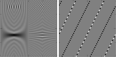
FIG. 4.: Diffraction effects in the Wigner propagation. Horizontal (vertical) axis correspond to position (momentum) basis. In the left plot we show the resulting Wigner function obtained by applying the operator $U_{FT}^{(N/2)}$ (corresponding to a Bernoulli shift) to a computational state. The classical propagation would contract and rotate the line shown in Fig.2, but the quantum propagation shows strong diffraction effects. In the right we show the result of propagating the same initial state with the ‘cat’ map (equation (56)). In this case the Wigner function evolves classically and shows no diffraction effects.

F Quantum algorithms in phase space

Quantum algorithms are nothing but unitary operators that have been designed so that after applying them several times, they produce a state that encodes the answer to some computational problem. A measurement on such state gives us information about this answer. Quantum algorithms are designed in such a way that they have a regular behavior as function of $N$. Thus, at least in some cases, one should be able to observe this regularities in a phase space representation. In fact, such representation becomes more useful also in the large $N$ limit, which is the semiclassical limit (since $1/N$ is an effective Planck constant). The study of the phase space representation of quantum algorithms is only beginning but there are already some interesting results showing that some algorithms may find phase space as a natural arena to be represented in. The example we would like to point out here is Grover’s search algorithm whose phase space representation is shown in Figure 5

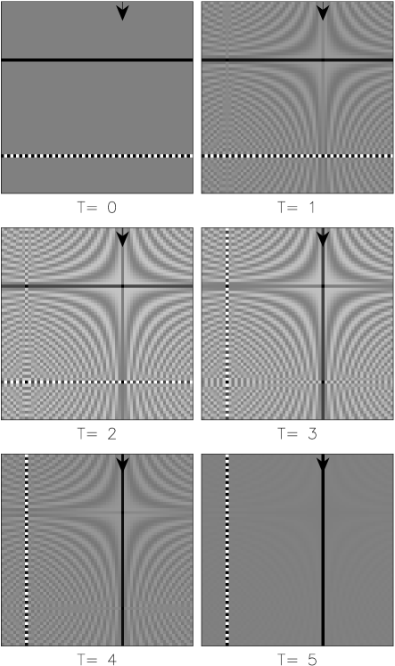
FIG. 5.: Grover’s algorithm in phase space. Horizontal (vertical) axis correspond to position (momentum) basis. After only five iterations the initial state (a momentum eigenstate) is transformed into a position eigenstate located precisely at the position of the marked item (see text).

In this Figure we display the Wigner function of the quantum state of a computer after every iteration of Grover’s search algorithm. Our system has an $N=32$–dimensional Hilbert space (i.e., the computer has just $5$ qubits) and the algorithm is designed to search for the marked item which we chose here to be $q=16$ (indicated with an arrow in the plot). The initial state is chosen to be an equally weighted superposition of all computational states which, for the purpose of making the plots more visible, we chose to be a non-zero momentum state (the usual choice for the initial state in Grover’s algorithm is a zero momentum state but the algorithm works as well with an initial state $|k\rangle$ with nonzero momentum). The quantum search algorithm consists of the iteration of a unitary operator $U_{G}$ which can be decomposed as $U_{G}=U_{k}U_{o}$. The operator $U_{o}$ represents a call to an oracle that only distinguishes the marked item $\omega$ from the rest: $U_{o}=I-2|\omega\rangle\langle\omega|$. The operator $U_{k}$ (the inversion about the mean) has no information about the marked item and is chosen as $U_{k}=I-2|k\rangle\langle k|$. The quantum computer should be initially prepared in the state $|k\rangle$. After a number of iterations $T\approx\pi\sqrt{N}/4$ the probability of detecting the position $q=\omega$ becomes of order unity (with small correction decaying as $1/N$). Thus, by measuring the position at this time one would discover the marked item. From the figure one clearly observes that this algorithm is very simple when seen from a phase space representation. The initial state has a Wigner function which is a horizontal strip (with its oscillatory companion). After each iteration $W(q,p)$ shows a very simple Fourier-like pattern and becomes a pure coordinate state at the end of the search (in our case, the optimal number of iterations is $T\approx\pi\sqrt{N}/4\approx 5$). This representation shows that, as a map, Grover’s algorithm has a fixed phase space point with coordinate equal to the marked item ($q=16$ in our case) and momentum equal to the one of the initial state.

It is interesting to speculate if this phase space representation may be of guidance to create new quantum algorithms or improve on existing ones. We cannot present clear evidence to support this but we believe this will be the case. However, some careful thought is required. At this moment we can only offer the reader some of our experience on the way one should not proceed: Viewing Figure 5 one may be tempted to try to find a quantum map that has the same fixed point as the above but transform horizontal strips into vertical ones faster than Grover’s. It is interesting to notice that such maps do exist. In fact, one just needs a hyperbolic (instead of an integrable) map with the same fixed point structure. In fact, a hyperbolic map with the same fixed point structure would perform the same operation exponentially faster, because it would transform a state initially along the stable direction into one along the unstable one in a time of order $\log(N)$ . Such hyperbolic maps can be easily constructed as variations of the quantum bakers map. However, their construction requires from the oracle much more information than a simple yes/no query and thus do not qualify as fast search algorithms.

VI Measuring the Wigner Function

In this section we review a general procedure to directly measure the value of the Wigner function of a system in any phase space point (the procedure applies for discrete and also for continuous systems). This measurement strategy was originally proposed in [21] as an application of a very general tomographic scheme. It generalizes previous proposals that were put forward to measure the Wigner function in quantum optics or cavity QED setups (see [3] for a review).

The basic idea of the measurement is best described in terms of the quantum algorithm represented by the simple quantum circuit shown in Figure 6. It works as follows: Suppose you want to measure the Wigner function of a system that is prepared in some quantum state $\hat{\rho}$. What you need to do is to bring this system in contact with an ancillary qbit prepared in the state $|0\rangle$ and then “run” the quantum computation described by the circuit shown in Figure 6. The ancillary qbit plays the role of a “probe particle” in a scattering–like experiment. The algorithm represented in the circuit is: i) Apply an Hadamard transform to the ancillary qbit (where $H|0\rangle=(|0\rangle+|1\rangle)/\sqrt{2}$, $H|1\rangle=(|0\rangle-|1\rangle)/\sqrt{2}$), ii) Apply a “controlled–$\hat{U}$” operator (if the ancilla is in state $|0\rangle$ this operator acts as the identity for the system but if the state of the ancilla is $|1\rangle$ it acts as the unitary operator $\hat{U}$ on the system), iii) Apply another Hadamard gate to the ancilla and finally perform a weak measurement on this qbit detecting its polarization (i.e., measuring the expectation values of Pauli operators $\sigma_{z}$ and $\sigma_{x}$). It is easy to show that the above circuit has the following remarkable property:

$$\langle\sigma_{z}\rangle=Re(Tr(\hat{U}\hat{\rho})),\quad\langle\sigma_{y}\rangle=-Im(Tr(\hat{U}\hat{\rho})).$$ (65)

Thus, the final polarization measurement reveals a property determined both by the initial state $\hat{\rho}$ and the unitary operator $\hat{U}$.

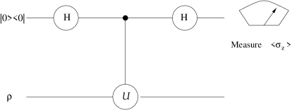
FIG. 6.: Circuit for measuring $Re(Tr(U\rho))$, for a given unitary operator $U$.

It is clear that this circuit can be used for dual purposes: On the one hand, we can use it to extract information on the operator $\hat{U}$ if we know the state $\hat{\rho}$. On the other hand, the same circuit can be used to learn about the state $\hat{\rho}$ by using some specific operators for $\hat{U}$. In this sense, this circuit can be adapted to act either as a tomographer or as an spectrometer which, therefore, are two dual faces of the simple quantum computation shown above [21]. The analogy with a typical scattering experiment is quite clear: the probe particle is prepared in a well determined state, then it interacts with the system. From the measurement of some statistical distribution of the probe (in this case the polarization) we are able to infer properties of either the interaction or the state of the scatterer.

In [21] we showed that this circuits can be used to measure the Wigner function. This is done by simply choosing $\hat{U}=\hat{A}(\alpha)$. By doing this, every time one runs the algorithm a direct measurement of $W(\alpha)$ is obtained (for any given phase space point $\alpha$). This measurement strategy can be, in principle, used both for the continuous and the discrete case. For example, in the continuous case, to measure $W(\alpha)$ of a quantum particle one has to run the algorithm with the system in the initial state $D(\alpha)\hat{\rho}D^{\dagger}(\alpha)$ (obtained by displacing $\hat{\rho}$) and using $\hat{U}=\hat{R}$ (it is clear that this is equivalent, but simpler, than applying the circuit directly with $\hat{U}=\hat{A}(\alpha)$). The measurement of the Wigner function for the discrete case can be done in a similar way but in that case it is more convenient to directly use $\hat{U}=\hat{A}(\alpha)$. In both cases, as the operator $\hat{A}(\alpha)$ is both unitary and hermitian, the measurement of the Wigner function only requires determining the $z$–component of the polarization.

Measuring directly the Wigner function of a quantum system has been the goal of a series of experiments proposed and performed in various areas of physics (all dealing with continuous systems, [22]). It is interesting to notice that the above measurement strategy precisely describes the experiment recently performed to determine the Wigner function of the electromagnetic field in a cavity QED setup [23, 24]. In fact, in such case the system is the mode of the field stored in a high–$Q$ cavity and the ancillary qbit is a two level atom. Remarkably, this experiment can be easily described in terms of the application of the algorithm shown in Figure 6: i) The atom goes through a Ramsey zone that has the effect of implementing an Hadammard transform. A radio-frequency source is connected to the cavity displacing the field in phase space (by an amount parametrized by $\alpha$), ii) The atom goes through the cavity interacting dispersively with the field. The interaction is tuned in such a way that, if the atom is in state $|g\rangle$ nothing happens but if the state of the atom is $|e\rangle$ the state acquires a phase shift of $\pi$ per photon in the cavity. So, this interaction is simply a controlled–$\exp(-i\pi\hat{N})$ gate (where $\hat{N}$ is the photon number operator) which is nothing but a controlled reflection. iii) The atom leaves the cavity entering a new Ramsey zone that enforces a new H–gate. Finally the atom is detected in a counter either in the ground $|g\rangle$ or in the excited $|e\rangle$ state. The experiment is repeated many times and the Wigner function is obtained as the difference between the probability of the atom being in the excited and ground states: $W(q,p)=2(P(e)-P(g))/\hbar$. As we see, this cavity–QED experiment is an example of a tomographic experiment represented by the circuit of Figure 6. The important point is that the method is generalizable to arbitrary systems (continuous or discrete) when viewed in terms of the above circuit.

For the discrete case, one can show that the circuit in Figure 6 can be efficiently decomposed as a sequence of elementary gates. For this, one only needs to implement controlled-$\tilde{U}$, $\tilde{V}$ and $\hat{R}$ operations. All these can be implemented via efficient networks like the ones shown in [25] which require a number of elementary gates that depends polinomially on $log(N)$. For example, to decompose $\hat{V}$ as a sequence of one qbit gates we can notice that its action on a computational state $|n\rangle$ is:

$$\hat{V}^{p}|n\rangle=\prod_{i=0}^{L-1}\left[\exp(i2\pi p2^{i}/N)\right]^{n_{i}}|n\rangle$$ (66)

where $n_{i}$ is the binary expansion of the number $n$. From this expression it is clear that to implement $\hat{V}$ we just have to act independently on each qbit. The operator $\phi_{i}$ acting on the i–th qbit should be such that $\phi_{i}|0\rangle=|0\rangle$ and $\phi_{i}|1\rangle=\exp(i2\pi p2^{i}/N)|1\rangle$. On the other hand, to implement $\hat{U}$, which is a shift in the position basis, we can either use a circuit which performs addition mod $N$ as described in [25] or notice that a circuit for $\hat{U}$ is obtained from the one corresponding to $\hat{V}$ by using $\hat{U}=U_{FT}^{-1}\hat{V}U_{FT}$. Finally, to implement the reflection operator we use the identity (20) which states that two Fourier transforms are equivalent to a reflection. Therefore, the complete network can be obtained straightforwardly.

For small values of $N$ the resulting networks are indeed very simple. In [21] we have presented the results of the measurement of the Wigner function for the particular case of $N=4$ (two qbits) for a variety of initial states. In this case the reflection operator is simply a controlled not (CNOT) gate (where the control is in the least significant qbit). The circuit for $\hat{U}$ is the same CNOT followed by bit flip in the control. Analogously, the circuit for $\hat{V}$ is a sequence of controlled phase gates. Thus, the complete measurement circuit has at most one Tofolli gate and several two qbit gates. We experimentally measured the Wigner function of the four computational states of a two qbit quantum computer. The ideal result is shown in Figure 2 and the measured Wigner functions are seen in 7.

To perform these experiments we used a liquid sample of trichloroethylene (TCE) dissolved in chloroform. This molecule has been used in several three qubit experiments where the proton ($H$) and two strongly coupled ${}^{13}C$ nuclei ($C_{1}$ and $C_{2}$) store the three qbits [26]. In our case, we used $C_{1}$ as our control qbit (the probe particle in Figure 6) and the pair $H$-$C_{2}$ to store the state whose Wigner function we tomographically measure. The measured coupling constants are $J_{HC_{1}}=200.76\ \mbox{Hz}$, $J_{HC_{2}}=9.12\ \mbox{Hz}$ and $J_{C_{1}C_{2}}=103.06\ \mbox{Hz}$ while the $C_{1}$-$C_{2}$ chemical shift is $\delta_{C_{1}C_{2}}=908.88\ \mbox{Hz}$. To evaluate the Wigner function in each of the independent $16$ phase space points we expressed the algorithm of Figure 6 as a sequence of r.f. pulses and delays (the number of pulses in each sequence depends on the phase space points and varies between $5$–$20$ and take at most $100$ms to execute ($\ll T_{1},T_{2}$ of our sample)). Experiments were done at room temperature and we used temporal averaging to distill the initial pseudo-pure states [27]. The experiments were done on a standard $500$Mhz NMR spectrometer (Bruker AM-500 at LANAIS in Buenos Aires and DRX-500 at Los Alamos). We used a $5$mm probe tuned to ${}^{13}C$ and ${}^{1}H$ frequencies of $125.77$ MHz and $500.13$ Mhz, respectively. The measured Wigner functions shown in figure 7 agree with the ideal one within (in the worst case) approximately $15\%$ error. The most important sources of errors are understood and come from the effects of strong coupling (that alter the behavior of our gates) and numerical uncertainty in integrating the spectra. It is clear that the result of this simple experiment, that illustrate the tomographic measurement of a discrete Wigner function, agrees very well with the theoretical expectation.

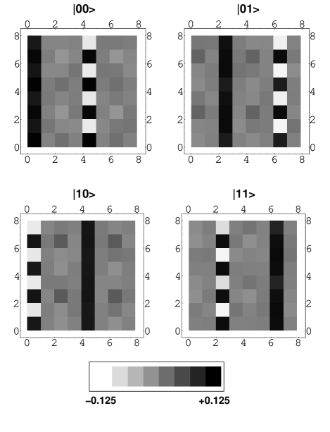
FIG. 7.: Measured Wigner functions for the four computational states of a two–qbit system (built with a liquid sample of TCE in an NMR spectrometer). Horizontal (vertical) axis correspond to position (momentum) basis. Ideally, these Wigner functions should be nonzero only on two vertical strips where they take values which are $\pm 1/8$. Experimental results show small deviations from these values (with a maximum error of $15\%$.

VII Conclusion

In this paper we first reviewed the formalism to represent in phase space the states and the evolution of a quantum system with a finite dimensional Hilbert space. Then, we applied this formalism to study the phase space representation of quantum computers and quantum algorithms. Finally, we discussed how to perform direct measurements to determine the Wigner function. Our approach, based on the use of phase space point operators to define the Wigner function enables us to find simple proofs for a variety of old and new results concerning both states and algorithms.

The differences between quantum and classical evolution in phase space are clearly seen using this phase space representation: For the Wigner function to evolve classically it is necessary (and sufficient) that the phase space point operators are transformed by the unitary evolution operator in the same way that classical evolution maps phase space points. In our paper we described a rather interesting family of operators with this property. It contains all linear homeomorphisms in the torus (i.e., the family of all “cat” maps) which can be efficiently represented by simple quantum circuits (since they correspond to kicked systems where kinetic and potential terms act alternatively). Moreover, this family also includes all cyclic shifts in the computational (or the momentum) basis, reflections and the Fourier transform. At a deeper level all these properties are a consequence of the well known invariance of the Wigner function under the action of the unitary representation of linear canonical transformations (that form the metaplectic group). Other unitary maps, that have a definite classical non–linear counterpart, will display for some time an almost classical behavior, signalled by a sharply peaked $Z_{\alpha\beta}$ matrix. This is the semiclassical limit, that will be reached in the limit $N\to\infty$, which is an important regime for interesting quantum algorithms since it corresponds to the limit of large number of qubits. A much wider category of maps can display a more drastic wave phenomenon: strong diffraction due to discontinuities. Consider, as the simplest example the phase space operation of a control-$U$ gate. The controlling qubit divides phase space in two disjoint regions and the $U$-gate acting on the remaining qubits affects these two regions differently. In this sense it acts as a prism or a screen in an optical system. Another simple example of this sort is the action of the operator $U_{FT}^{N/2}$, that does not act on the most significant qbit but applies the Fourier transform to the rest (the diffraction effects are clearly seen in Figure 4). The implications and usefulness of these semiclassical features in quantum algorithms remain largely unexplored and will be the subject of further investigation [28].

- [1] M. Hillery, R.F. O’Connell, M.O. Scully, E. P. Wigner, Phys. Rep.106 (1984), 121.
- [2] P. Bianucci, C. Miquel, J. P. Paz and M. Saraceno, Discrete Wigner functions and the phase space representation of a quantum computer quant-ph/0105091, submitted to PRL (2000).
- [3] L. Davidovich Quantum optics in cavities, phase space representations and the classical limit of quantum mechanics, in New perspectives on quantum mechanics. AIP Conf. Proc. 464, ed S. Hacyan et al. (1999, New York, AIP); also in Proccedings of the First PASI Conference on Chaos, Decoherence and Entanglement; (2000) available at http://kaiken.df.uba.ar.
- [4] see for example W. H. Zurek, Physics Today 44, (1991) N 10, 36; (1994) 2508; J. P. Paz, S. Habib and W. H. Zurek, Phys. Rev. D47 (1992) 488.
- [5] see J. P. Paz and W. H. Zurek, “Environment induced superselection and the transition from quantum to classical; (2001). in “Coherent matter waves, Les Houches Session LXXII;, edited by R Kaiser, C Westbrook and F David, EDP Sciences, Springer Verlag (Berlin) (2001) 533-614 and references therein.
- [6] ”Quantum Information and Computation”, I. Chuang and M. Nielsen (2000), Cambridge University Press.
- [7] W. K. Wooters, Ann. Phys. NY 176 (1987), 1
- [8] U.Leonhardt, Phys. Rev. Lett. 74, 4101 (1995). U.Leonhardt, Pys. Rev. A 53, 2998 (1996).
- [9] J. H. Hannay, M. V. Berry, Physica 1D, 267 (1980)
- [10] A. Rivas, A. M. Ozorio de Almeida, Ann.Phys. 276 (1999), 123
- [11] A. Bouzouina, S. De Bievre, Comm. Math. Phys. 178 (1996)83
- [12] J.Bertrand and P.Bertrand, Found. Phys. 17 (1987) 397.
- [13] U.Fano, Review of Modern Physics, 29 (1957) 75.
- [14] J. Schwinger, Proc. Nat. Acad, Sci.46 (1960), 570, 893.
- [15] J. P. Paz and M. Saraceno, (2001) in progress.
- [16] V.I. Arnold and A. Avez, Ergodic Problems in Classical Mechanics, Benjamin, New York, (1968).
- [17] B. Georgeot and D. L. Shepelyansky, Phys. Rev. Lett. 86 (2001) 2890-2893; see also B. Georgeot and D. L. Shepelyansky, Phys. Rev. Lett. 86 (2001) 5393-5396.
- [18] N.L. Balasz and A. Voros, Ann. Phys. 190 (1990) 1.
- [19] A. Voros y M. Saraceno, Physica D79 (1994) 206; see also M. Saraceno, Ann. Phys. 199 (1990) 37.
- [20] R. Schack, Phys. Rev A57 (1998) 1634-1635; R. Schack and T. Brun, Phys. Rev. A 59 (1999) 2649-2658; see also R. Schack and Caves C. M., Appl. Algebr. Eng. Comm. 10 (2000) 305-310; A. N. Soklakov and R. Schack, Phys. Rev. E 61 (2000) 5108-5114.
- [21] C. Miquel, J.P. Paz, M. Saraceno, E. Knill, R. Laflamme, C. Negrevergne (2001) submitted to Nature.
- [22] T. J. Dunn et al., Phys. Rev. Lett. 74 (1994) 884; D. Leibfried et al. Phys. Rev. Lett. 77 (1996) 4281; see also Physics Today 51 no. 4 (1998) 22.
- [23] L. G. Lutterbach and L. Davidovich, Phys. Rev. Lett. 78 (1997) 2547; Optics Express 3 (1998) 147.
- [24] G. Nogues et al, Phys. Rev. A (2000); see also X. Maitre et al, Phys. Rev. Lett. 79 (1997) 769.
- [25] C.Miquel, J.P.Paz, R.Perazzo, Phys. Rev. A 54 (1996) 2605.
- [26] see for example: M. A. Nielsen, E. Knill, R. Laflamme, Nature 396 (1998), 52–55; D. G. Cory et al., Phys. Rev. Lett. 81 (1998) 2152
- [27] E.Knill, I.Chuang and R.Laflamme, Phys. Rev. A 57 3348.
- [28] J. P. Paz and M. Saraceno, (2001) work in progress.