Approximate Master Equations for Atom Optics

Abstract

In the field of atom optics, the basis of many experiments is a two level atom coupled to a light field. The evolution of this system is governed by a master equation. The irreversible components of this master equation describe the spontaneous emission of photons from the atom. For many applications, it is necessary to minimize the effect of this irreversible evolution. This can be achieved by having a far detuned light field. The drawback of this regime is that making the detuning very large makes the time step required to solve the master equation very small, much smaller than the time scale of any significant evolution. This makes the problem very numerically intensive. For this reason, approximations are used to simulate the master equation which are more numerically tractable to solve. This paper analyses four approximations: The standard adiabatic approximation; a more sophisticated adiabatic approximation (not used before); a secular approximation; and a fully quantum dressed-state approximation. The advantages and disadvantages of each are investigated with respect to accuracy, complexity and the resources required to simulate. In a parameter regime of particular experimental interest, only the sophisticated adiabatic and dressed-state approximations agree well with the exact evolution.

I The Master Equation

Many investigations in the realm of quantum physics are based on a single two level atom coupled to an approximately resonant light field. One major aspect of this work is to investigate the quantum mechanical motion of such an atom. The work of Steck et al Steck is a prime example. They investigate chaos assisted tunneling by studying the motion of cold cesium atoms in an amplitude modulated standing wave of light. Haycock et al Haycock study cesium atoms in an effort to observe quantum coherent dynamics. The work of Hensinger et al investigates quantum chaos Hen01a and quantum tunneling Hen01b . Proposals in QED to utilize interactions between atoms and their cavity for physical realizations of a quantum computer Pellizzari and for communication of quantum states Cirac also require good descriptions of quantum mechanical motion.

The full quantum system here consists of the light field and the atom. The evolution of such a system is governed by a Schrödinger equation. In most cases however, the evolution of the light field is not of interest and so the Schrödinger equation can be reduced to a master equation. The most general form of this master equation is given by

$$\dot{\rho}=-\frac{i}{\hbar}\left[H,\rho\right]+\mathcal{L}\rho,$$ (1)

where $\mathcal{L}$ is a Lindbladian superoperator Lind .

The form we will use here, specific to a two level atom interacting with a light field, is

$$H=\frac{p_{x}^{2}}{2m}+\hbar\delta\sigma^{\dagger}\sigma+\frac{\hbar}{2}\left[\Omega(x,t)\sigma^{\dagger}+\Omega^{\dagger}(x,t)\sigma\right],$$ (2a)

$$\mathcal{L}\rho=\Gamma\left(\mathcal{B}\mathcal{J}\left[\sigma\right]\rho-\mathcal{A}\left[\sigma\right]\rho\right).$$ (2b)

Here we are only interested in the motion of the atom in the one direction. Thus $p_{x}$ is the component of the atom’s momentum in the $x$-direction. The detuning of the light field is $\delta$. The atomic lowering operator is given by $\sigma=|{g}\rangle\langle{e}|$ where $|{g}\rangle$ and $|{e}\rangle$ represent the ground and excited states of the atom respectively. $\Omega(x,t)$ is the complex, and possibly time-dependent Rabi frequency operator for the light field, which, from here on, will be represented simply as $\Omega$. $k$ and $m$ are the wavenumber of the incident photons and the mass of the atom respectively. Planck’s constant ($\hbar$) will be set to one for the rest of the analysis. The superoperator $\mathcal{B}$ describes random momentum kicks. It is defined for any arbitrary operator $a$ as

$$\mathcal{B}a=\int_{-1}^{1}W(u)e^{ikux}ae^{-ikux}du,$$ (3)

where $W(u)$ is the atomic dipole radiation distribution function produced by the electronic transition, reduced to one dimension Hen01a . For motion parallel to the direction of propagation of the laser light, it is given by

$$W(u)=\frac{3}{8}\left(1+u^{2}\right).$$ (4)

The superoperators $\mathcal{J}$ and $\mathcal{A}$ are defined for arbitrary operators $c$ and $a$ as

$$\mathcal{J}\left[c\right]a=cac^{\dagger},\mathcal{A}\left[c\right]a=\frac{1}{2}\left\{c^{\dagger}c,a\right\},$$ (5)

and define the general form of a Lindbladian Lind superoperator.

The entire expression of Eq. (2b) describes the irreversible evolution of the system at rate $\Gamma$. It is this part of the master equation that we wish to minimize by working in the regime $\delta\gg\Omega_{\mathrm{max}}\gg\Gamma$ (where $\Omega_{\mathrm{max}}$ is the maximum modulus of the Rabi frequency operator). The problem with this regime is that when making $\delta$ very large, the full master equation still has to be solved using a timestep smaller than $\delta^{-1}$. This makes solving the full master equation numerically very difficult.

There are a number of ways to approximate the master equation, four of which are investigated here. These are

1. The standard adiabatic approximation;

2. A more sophisticated adiabatic approximation;

3. A secular approximation; and

4. A dressed-state approximation.

Approximation (1) is a standard approach used by many researchers in the field, both as a semi-classical treatment Parkins and as a fully quantum approximation method Hen01a ; Graham . Unfortunately, this treatment is not valid in the regime of the work of Hen01a . These experiments were performed in the regime of $\delta\gg\Omega_{\mathrm{max}}\gg\Gamma$ but where $\Gamma$ is the same order as $\Omega^{2}_{\mathrm{max}}/\delta$. In their work, approximation (1) was used but on closer examination, this approximation was seen only to be valid in the regime $\Gamma\gg\Omega^{2}_{\mathrm{max}}/\delta$. We will concentrate on the difficult $(\Gamma\sim\Omega^{2}_{\mathrm{max}}/\delta)$ regime in this analysis. Approximation (2) is one way to correct the standard adiabatic approximation for this regime. Approximation (3) was proposed in Ref. dyrtingmilburn , and was used for the formation of quantum trajectory simulations in Ref.Hen01a . Approximation (4) is a fully quantum dressed-state treatment including the effect of spontaneous emission. Previously, only semi-classical treatments, both omitting Deutschmann , and including Dalibard ; Parkins , spontaneous emission have been done. We look at all four approximations, examining the validity and complexity, as well as the numerical accuracy (compared to the full simulation) and computational resource requirements, of each.

II The standard adiabatic approximation

The method of adiabatic approximation applied to the full master equation serves to eliminate the internal state structure of the atom. One reason for wishing to have no internal states is so that the system has a clear classical analogue dyrtingmilburn . In performing this treatment, we also remove the Hamiltonian term of order $\delta$, removing the requirement that the master equation be solved on a timestep at least as small as $\delta^{-1}$. This adiabatic elimination technique is described in many different text books, see Meystre ; Barnett . The result we obtain was first derived by Graham, Schlautmann and Zoller Graham . To achieve this adiabatic elimination however, we follow a procedure similar to that of Hensinger et al Hen01a .

The density matrix can be written using the internal state basis as

$$\rho = \rho_{gg}\otimes|{g}\rangle\langle{g}|+\rho_{ge}\otimes|{g}\rangle\langle{e}|$$ (6)

$$\rho^{\dagger}_{ge}\otimes|{e}\rangle\langle{g}|+\rho_{ee}\otimes|{e}\rangle\langle{e}|,$$

where the $\rho_{gg}$ etc are still operators on the centre-of-mass Hilbert space L${}^{(2)}(\mathbb{R})$. From Eqs. (2), these obey

$$\dot{\rho}_{gg} = \Gamma\mathcal{B}\rho_{ee}-\frac{i}{2}\left(\Omega^{\dagger}\rho_{eg}-\rho_{ge}\Omega\right)-\mathcal{K}\rho_{gg},$$ (7a)

$$\dot{\rho}_{ge} = -\frac{\Gamma}{2}\rho_{ge}-\frac{i}{2}\left(\Omega^{\dagger}\rho_{ee}-\rho_{gg}\Omega^{\dagger}\right)+i\delta\rho_{ge}$$ (7b)

$$-\mathcal{K}\rho_{ge},$$

$$\dot{\rho}_{ee} = -\Gamma\rho_{ee}-\frac{i}{2}\left(\Omega\rho_{ge}-\rho_{eg}\Omega^{\dagger}\right)-\mathcal{K}\rho_{ee}.$$ (7c)

Here the kinetic energy term is represented in the superoperator

$$\mathcal{K}\rho=i\left[\frac{p_{x}^{2}}{2m},\rho\right].$$ (8)

If the standard adiabatic elimination procedure is valid, we can represent the system by the density matrix for the centre of mass (com) alone,

$$\rho_{\rm com}={\rm Tr_{int}}[\rho]=\rho_{gg}+\rho_{ee},$$ (9)

where ${\rm Tr_{int}}$ is the trace over the internal states of the atom. In this standard adiabatic approximation we further simplify this by noting that large detuning leads to very small excited state populations such that $\rho_{gg}\gg\rho_{ee}$ and thus $\rho_{\rm com}$ is approximately $\rho_{gg}$. Thus denoting $\rho_{\rm com}$ simply as $\rho$, we can replace $\rho_{gg}$ in Eq. (7a) just with $\rho$.

Now we require expressions for $\rho_{ge}$ and $\rho_{ee}$ in terms of $\rho$. This is achieved by noting that from Eq. (7b), $\rho_{ge}$ comes to equilibrium on a timescale much shorter than $\rho_{gg}$, at a rate $\Gamma/2$. Thus we set $\dot{\rho}_{ge}=0$. Also, if the kinetic energy term is much smaller than $\delta$ then it can be ignored. This will be the case if $\delta\gg\langle p_{x}^{2}/m\rangle$. This is typically true, and so we get

$$\rho_{ge}=i\frac{\rho_{gg}\Omega^{\dagger}-\Omega^{\dagger}\rho_{ee}}{\Gamma-2i\delta}.$$ (10)

This can be substituted back into the equation for $\rho_{ee}$ to give

$$\dot{\rho}_{ee} = -\Gamma\left(\rho_{ee}+\frac{\left\{\Omega\Omega^{\dagger},\rho_{ee}\right\}}{2\left(\Gamma^{2}+4\delta^{2}\right)}+\frac{i\delta\left[\Omega\Omega^{\dagger},\rho_{ee}\right]}{\Gamma\left(\Gamma^{2}+4\delta^{2}\right)}\right)$$ (11)

$$+\frac{\Gamma\mathcal{J}\left[\Omega\right]\rho_{gg}}{\Gamma^{2}+4\delta^{2}}-\mathcal{K}\rho_{ee}.$$

From Eq. (11), we see that $\rho_{ee}$ equilibrates on a timescale much faster than $\rho_{gg}$ and so we also set $\dot{\rho}_{ee}=0$. This time, the kinetic energy term must be ignored compared with $\Gamma$ rather than $\delta$. Allowing this approximation gives

$$\rho_{ee}+\frac{\left\{\Omega\Omega^{\dagger},\rho_{ee}\right\}}{2\left(\Gamma^{2}+4\delta^{2}\right)}+\frac{i\delta\left[\Omega\Omega^{\dagger},\rho_{ee}\right]}{\Gamma\left(\Gamma^{2}+4\delta^{2}\right)}\simeq\frac{\Omega\rho_{gg}\Omega^{\dagger}}{\Gamma^{2}+4\delta^{2}}.$$ (12)

The first correction term on the left hand side scales as $(\Omega/\delta)^{2}$ which in the regime chosen is negligible compared to the leading order term. The second correction term however scales as $\left(\Omega^{2}/\delta\right)/\Gamma$. Had we been working in the regime $\Gamma\gg\Omega^{2}/\delta$, then this term could also be safely ignored compared to the leading term. This condition however, is not satisfied in the experiments of Hen01a nor in our chosen regime, leaving this term the same order as the leading term. This term however was dropped in Ref. Hen01a on the basis that in a more sophisticated approach (Sec. III), this term does not appear and the correction to the final master equation is small Hen01a . Knowing that this is an unjustified approximation, but in the interest of comparison to currently used techniques Hen01a , we will continue to follow this method as others have done. Thus, dropping the second correction term we are left with

$$\rho_{ee}\simeq\frac{\Omega\rho_{gg}\Omega^{\dagger}}{\Gamma^{2}+4\delta^{2}}.$$ (13)

Now substituting first Eq. (10) then Eq. (13) into Eq. (7a) and replacing $\rho_{gg}$ with $\rho$ gives the final adiabatically eliminated master equation:

$$\dot{\rho} = \Gamma\left(\mathcal{B}\mathcal{J}\left[\frac{\Omega}{2\delta}\right]\rho-\mathcal{A}\left[\frac{\Omega}{2\delta}\right]\rho\right)-i\left[\frac{p_{x}^{2}}{2m}-\frac{\Omega\Omega^{\dagger}}{4\delta},\rho\right],$$

where here we have used the fact that $\delta\gg\Omega\gg\Gamma$ to eliminate some of the higher order terms. This master equation is of the Lindblad form.

III A more sophisticated Adiabatic approximation

As noted, the standard adiabatic elimination method described in section II is not strictly valid in the regime of the experiments of Hensinger et al Hen01a , $\Gamma\sim\Omega_{\mathrm{max}}^{2}/\delta$. There are a number of ways to try and develop a strictly valid version of the adiabatic approximation in this regime. One way would be to not drop any terms without justification and continue to plough through the mathematics. Another method which we believe to be neater and just as accurate is proposed here by using a slightly more sophisticated method similar to that in the appendix of howpolly .

The basis of the approach is to move into an interaction picture with respect to

$$H_{0}=\frac{\Omega\Omega^{\dagger}}{4\delta}.$$ (15)

This approach may seem counter-intuitive to most. Usually when moving to an interaction picture, it would be with respect to a $H_{0}$ that is already one of the terms in the Hamiltonian. In our case, if we investigate Eq. (LABEL:adiab1me), we are moving to an interaction picture with respect to the opposite of a term in the effective Hamiltonian and as such will actually be adding a term to the Hamiltonian. The reason we choose to do this is that the problem term we encountered in Sec. II was in the Hamiltonian for the excited state. The potential seen by the excited state of the atom is in fact inverted and so the chosen $H_{0}$ is designed to cancel the excited state potential.

After moving into this interaction picture, we then perform the adiabatic elimination process, and finally transform back into the Schrödinger picture. This method can give a different result because the approximations we make in the interaction picture may not have been valid in the Schrödinger picture.

With the unitary transformation operator $U_{0}(t)=e^{-iH_{0}t}$, the interaction picture density matrix is

$$\tilde{\rho}=U^{\dagger}_{0}(t)\rho U_{0}(t).$$ (16)

Using this in Eqs. (2) gives an interaction picture master equation equation still of the Lindblad form

$$\dot{\tilde{\rho}}=-i\left[\tilde{V},\tilde{\rho}\right]+\Gamma\mathcal{L}\tilde{\rho},$$ (17)

but now with an extra Hamiltonian term such that $\tilde{V}$ is given by

$$\tilde{V}=\frac{\tilde{p}_{x}^{2}}{2m} + \delta\sigma^{\dagger}\sigma+\frac{1}{2}\left(\Omega\sigma^{\dagger}+\Omega^{\dagger}\sigma\right)+\frac{\Omega\Omega^{\dagger}}{4\delta}.$$ (18)

Where $\tilde{p}_{x}$ is just the component of the momentum in the $x$-direction, transformed into the interaction picture. The Lindbladian superoperator $\mathcal{L}$ is unaffected by the interaction picture because Rabi frequency operator $\Omega$ commutes with the position operator, $x$, as well as with the state operators, $\sigma$ and $\sigma^{\dagger}$.

Following the same procedure as the standard adiabatic elimination process, the equations for the centre-of-mass operators can be extracted:

$$\dot{\tilde{\rho}}_{gg} = \Gamma\mathcal{B}\tilde{\rho}_{ee}-\frac{i}{2}\left(\Omega^{\dagger}\tilde{\rho}_{eg}-\tilde{\rho}_{ge}\Omega\right)-\frac{i}{4\delta}\left[\Omega\Omega^{\dagger},\tilde{\rho}_{gg}\right]$$ (19a)

$$-\tilde{\mathcal{K}}\tilde{\rho}_{gg},$$

$$\dot{\tilde{\rho}}_{ge} = -\frac{\Gamma}{2}\tilde{\rho}_{ge}-\frac{i}{2}\left(\Omega^{\dagger}\tilde{\rho}_{ee}-\tilde{\rho}_{gg}\Omega^{\dagger}\right)-\frac{i}{4\delta}\left[\Omega\Omega^{\dagger},\tilde{\rho}_{ge}\right]$$ (19b)

$$+i\delta\tilde{\rho}_{ge}-\tilde{\mathcal{K}}\tilde{\rho}_{ge},$$

$$\dot{\tilde{\rho}}_{ee} = -\Gamma\tilde{\rho}_{ee}-\frac{i}{2}\left(\Omega\tilde{\rho}_{ge}-\tilde{\rho}_{eg}\Omega^{\dagger}\right)-\frac{i}{4\delta}\left[\Omega\Omega^{\dagger},\tilde{\rho}_{ee}\right]$$ (19c)

$$-\tilde{\mathcal{K}}\tilde{\rho}_{ee},$$

where obviously $\tilde{\mathcal{K}}$ uses the interaction picture momentum operator $\tilde{p}_{x}$.

In this more sophisticated approach, we still take the trace over the internal states of the atom, letting $\tilde{\rho}_{\rm com}=\tilde{\rho}_{gg}+\tilde{\rho}_{ee}$, but now we do not simplify this further and simply let $\tilde{\rho}=\tilde{\rho}_{gg}+\tilde{\rho}_{ee}$. This gives a master equation of the form

$$\dot{\tilde{\rho}} = \Gamma\left(\mathcal{B}-1\right)\tilde{\rho}_{ee}-\frac{i}{2}\left[\Omega^{\dagger},\tilde{\rho}_{eg}\right]-\frac{i}{2}\left[\Omega,\tilde{\rho}_{ge}\right]$$ (20)

$$-\frac{i}{4\delta}\left[\Omega\Omega^{\dagger},\tilde{\rho}\right]-\tilde{\mathcal{K}}\tilde{\rho}.$$

Hence we again need to find expressions for $\tilde{\rho}_{ee}$ and $\tilde{\rho}_{ge}$ in terms of $\tilde{\rho}$. We can achieve this by noting that, as in the earlier treatment, $\tilde{\rho}_{ee}$ and $\tilde{\rho}_{ge}$ equilibrate on a timescale much faster than $\tilde{\rho}_{gg}$. By setting $\dot{\tilde{\rho}}_{ge}=0$, and again ignoring the kinetic energy term, we get

$$\tilde{\rho}_{ge} = -\frac{\tilde{\rho}\Omega^{\dagger}}{2\delta}-\frac{\left[\Omega\Omega^{\dagger},\tilde{\rho}\Omega^{\dagger}\right]}{8\delta^{3}}+\frac{\left\{\Omega^{\dagger},\tilde{\rho}_{ee}\right\}}{2\delta}-\frac{\Gamma\tilde{\rho}\Omega^{\dagger}}{4i\delta^{2}}$$ (21)

$$+\frac{\Gamma\left\{\Omega^{\dagger},\tilde{\rho}_{ee}\right\}}{4i\delta^{2}}+\frac{\left[\Omega\Omega^{\dagger},\left\{\Omega^{\dagger},\tilde{\rho}_{ee}\right\}\right]}{8\delta^{3}}.$$

Setting $\dot{\tilde{\rho}}_{ee}=0$ and ignoring the kinetic energy term allows us to solve for $\tilde{\rho}_{ee}$. In the more sophisticated adiabatic treatment, instead of getting an equation of the form of Eq. (12), we get

$$\mathcal{R}\tilde{\rho}_{ee}=\mathcal{F}\frac{\Omega\tilde{\rho}\Omega^{\dagger}}{4\delta^{2}}.$$ (22)

In Eq. (22), the superoperators $\mathcal{F}$ and $\mathcal{R}$ are defined

$$\mathcal{F} \equiv 1+\frac{i}{2\delta\Gamma}\left[\Omega\Omega^{\dagger},\ldots\right],$$ (23)

$$\mathcal{R} \equiv \mathcal{F}+\text{ higher order terms}.$$ (24)

In the regime chosen ($\Gamma\sim\Omega^{2}/\delta$), the second term of Eq. (23) is of order 1 and so cannot be ignored compared to the leading term. In Eq. (24), the higher order terms are of order much smaller than 1 and even smaller than $\Omega^{4}/\delta^{3}$, which is the smallest order kept by making Taylor approximations to get the expression for $\tilde{\rho}_{ge}$. Thus to simplify Eq. (22), we act on the left of both sides with the superoperator $\mathcal{F}^{-1}$. Then to leading order we have

$$\tilde{\rho}_{ee} \simeq \frac{\Omega\tilde{\rho}\Omega^{\dagger}}{4\delta^{2}}.$$ (25)

As expected, the interaction picture chosen produced a term in $\rho_{gg}$ to counteract the unwanted term in $\rho_{ee}$. Notice here that we come to essentially the same result as in the standard adiabatic treatment in Eq. (13) but without making any unjustified approximations.

Now substituting Eq. (21) and Eq. (25) into Eq. (20), after simplification, leads to the final interaction picture master equation

$$\dot{\tilde{\rho}} = \Gamma\left(\mathcal{B}\mathcal{J}\left[\frac{\Omega}{2\delta}\right]\tilde{\rho}-\mathcal{A}\left[\frac{\Omega}{2\delta}\right]\tilde{\rho}\right)-i\left[\frac{\Omega^{2}{\Omega^{\dagger}}^{2}}{16\delta^{3}},\tilde{\rho}\right]$$ (26)

$$-\tilde{\mathcal{K}}\tilde{\rho}.$$

Finally, all that remains is to transform the interaction picture master equation back to the Schrödinger picture by performing the opposite unitary transformation. This leaves the final master equation for the more sophisticated adiabatic elimination treatment as

$$\dot{\rho} = \Gamma\left(\mathcal{B}\mathcal{J}\left[\frac{\Omega}{2\delta}\right]\rho-\mathcal{A}\left[\frac{\Omega}{2\delta}\right]\rho\right)$$ (27)

$$-i\left[\frac{p_{x}^{2}}{2m}-\frac{\Omega\Omega^{\dagger}}{4\delta}+\frac{\Omega^{2}{\Omega^{\dagger}}^{2}}{16\delta^{3}},\rho\right].$$

Notice here that by explicitly accounting for the term in $\Omega^{2}/\Gamma\delta$, the master equation derived is the same as that of the standard adiabatic approach with an extra potential term of order $\Omega^{4}/\delta^{3}$. This term is very small and as such the statements made to justify the standard approach Hen01a were correct in that the adjustment to the final master equation is small. The more sophisticated treatment however, although more algebraically intensive to produce the initial master equation, requires very little extra effort than the standard adiabatic treatment to simulate. More importantly though, the master equation derived in the more sophisticated adiabatic approach is valid in the regime $\Omega_{\mathrm{max}}^{2}/\delta\sim\Gamma$.

IV A Secular Approximation

A secular approximation to the full master equation is quite different from any adiabatic approximation. A secular approximation does not totally remove any dependence on the internal state of the atom. It only eliminates the coherences between the internal atomic states. The secular approximation was also used by Hensinger et al Hen01a , alongside the standard adiabatic approximation.

There are a number of ways to derive a secular approximation to the full master equation. One such method has been performed by Dyrting and Milburn dyrtingmilburn but this method is quite complicated. A much simpler method which produces the same approximate master equation is based on the technique that is applied for the standard adiabatic approximation.

We start with the Eqs. (7) for $\rho_{gg}$ etc, and then adiabatically eliminate $\rho_{eg}$ as in Sec. II. However, instead of also trying to solve for $\rho_{ee}$, we just substitute the expression for $\rho_{ge}$, Eq. (10), into the equations for $\rho_{gg}$, Eq. (7a) and $\rho_{ee}$, Eq. (7c). This eliminates the coherences between the excited and ground states while still keeping much of the original master equation. One advantage of this is that it allows comparison to an analogous 2-state classical model dyrtingmilburn . More importantly to us, this approximation eliminates the evolution at rate $\delta$ as is necessary to simplify the simulations. We are left with the following equations for the ground and excited state density matrices

$$\dot{\rho}_{gg} = \Gamma\mathcal{B}\rho_{ee}+\Gamma\left(\mathcal{J}\left[\frac{\Omega^{\dagger}}{2\delta}\right]\rho_{ee}-\mathcal{A}\left[\frac{\Omega}{2\delta}\right]\rho_{gg}\right)$$ (28)

$$+i\left[\frac{\Omega\Omega^{\dagger}}{4\delta},\rho_{gg}\right]-\mathcal{K}\rho_{gg},$$

$$\dot{\rho}_{ee} = -\Gamma\rho_{ee}+\Gamma\left(\mathcal{J}\left[\frac{\Omega}{2\delta}\right]\rho_{gg}-\mathcal{A}\left[\frac{\Omega^{\dagger}}{2\delta}\right]\rho_{ee}\right)$$ (29)

$$-i\left[\frac{\Omega\Omega^{\dagger}}{4\delta},\rho_{ee}\right]-\mathcal{K}\rho_{ee}.$$

The final master equation is constructed by recombining the equations (28) and (29) to produce an equation which reproduces these equations for $\dot{\rho}_{gg}$ and $\dot{\rho}_{ee}$ while also only giving rapidly decaying terms for $\dot{\rho}_{ge}$ and $\dot{\rho}_{eg}$. This final master equation for the secular approximation is

$$\dot{\rho} = -i\left[\frac{p_{x}^{2}}{2m}+\frac{\Omega\Omega^{\dagger}}{4\delta}\sigma_{z},\rho\right]+\Gamma\left(\mathcal{B}\mathcal{J}\left[\sigma\right]\rho-\mathcal{A}\left[\sigma\right]\rho\right)$$ (30)

$$+\Gamma\left(\mathcal{J}\left[\frac{\Omega^{\dagger}\sigma}{2\delta}\right]\rho-\mathcal{A}\left[\frac{\Omega^{\dagger}\sigma}{2\delta}\right]\rho\right)$$

$$+\Gamma\left(\mathcal{J}\left[\frac{\Omega\sigma^{\dagger}}{2\delta}\right]\rho-\mathcal{A}\left[\frac{\Omega\sigma^{\dagger}}{2\delta}\right]\rho\right),$$

where $\sigma_{z}$ is just the Pauli spin operator $\sigma^{\dagger}\sigma-\sigma\sigma^{\dagger}$.

To compare this master equation with those we have already seen, the Hamiltonian terms derived here are the same as those derived in the standard adiabatic approximation, Eq. (LABEL:adiab1me). The spontaneous emission term exactly as in the full master equation, Eq. (2b), remains, while two extra jump terms involving a state change with no spontaneous emission have been derived.

There are no apparent problems in this derivation, or that in dyrtingmilburn . Nevertheless, as we will discuss in Sec VIII, Eq. (30) does not give accurate results in comparison with Eq. (1), in the regime $\Omega^{2}\sim\Gamma\delta$.

V A Dressed-State Approximation

A semi-classical dressed-state treatment of atomic motion was put forward by Dalibard and Cohen-Tannoudji Dalibard . The dressed-state approximation used here is a fully quantum version of that treatment.

The states we have been using for a basis so far, $|{g}\rangle$ and $|{e}\rangle$, are called bare states. We can also work with another basis of position-dependent states which we call dressed-states. These dressed-states are derived by considering the Hamiltonian of the full master equation Eq. (2a) and ignoring the kinetic energy component to get

$$V=\delta\sigma^{\dagger}\sigma+\mbox{$\frac{1}{2}$}\left(\Omega\sigma^{\dagger}+\Omega^{\dagger}\sigma\right).$$ (31)

The diagonalization of the Hamiltonian yields the form

$$V=E_{1}(x,t)a^{\dagger}a+E_{2}(x,t)aa^{\dagger},$$ (32)

where $E_{1}$ and $E_{2}$ are the eigenenergies of $V$. The corresponding eigenstates are the position dependent dressed-states we will be considering here, labeled $|{1}\rangle$ and $|{2}\rangle$. In terms of these dressed-states, $a$ is given by $|{2}\rangle\langle{1}|$. The energies and states are

$$E_{1}(x,t) = \mbox{$\frac{1}{2}$}\left(\delta+\Delta\right),$$ (33)

$$E_{2}(x,t) = \mbox{$\frac{1}{2}$}\left(\delta-\Delta\right),$$ (34)

$$|{1}\rangle = \sin{\theta}|{g}\rangle+\cos{\theta}|{e}\rangle,$$ (35)

$$|{2}\rangle = \cos{\theta}|{g}\rangle-\sin{\theta}|{e}\rangle,$$ (36)

where $\theta$ is defined by

$$\sin{\theta} = \frac{\Omega}{\sqrt{2}}\left(\delta^{2}+\delta\Delta+\Omega\Omega^{\dagger}\right)^{-\frac{1}{2}},$$ (37a)

$$\cos{\theta} = \frac{\Delta+\delta}{\sqrt{2}}\left(\delta^{2}+\delta\Delta+\Omega\Omega^{\dagger}\right)^{-\frac{1}{2}},$$ (37b)

and $\Delta=\left(\delta^{2}+\Omega\Omega^{\dagger}\right)^{\frac{1}{2}}.$

Now, we use this basis to get equations for $\rho_{11}$, $\rho_{12}$, $\rho_{21}$ and $\rho_{22}$. Without including the spontaneous emission or the kinetic energy, these equations are simply

$$\dot{\rho}_{jk}=-i\left[E_{j}(x,t)\rho_{jk}-\rho_{jk}E_{k}(x,t)\right].$$ (38)

We do however want to include the spontaneous emission in our treatment and so we must assess the effect of the raising and lowering operators for the bare states ($\sigma=|{g}\rangle\langle{e}|$ and $\sigma^{\dagger}=|{e}\rangle\langle{g}|$) acting on the new basis states ($|{1}\rangle$ and $|{2}\rangle$). This is easily done.

So far there have been no approximations made. The essence of the dressed-state approximation is similar to the secular approximation in that we keep the internal dressed-states but allow the coherences to go to zero. In contrast to the secular approximation, we do not simply set $\dot{\rho}_{12}=0$. Instead, we notice from Eq. (38) that, if we ignore the operator nature of the eigenenergies, then the equations for $\rho_{12}$ would have a term of the form $-i\left(E_{1}-E_{2}\right)\rho_{12}$. To first order, $E_{1}-E_{2}$ is approximately $\delta$. Thus $\rho_{12}$ will rotate very quickly such that only terms rotating at this very rapid pace will be able to contribute to its evolution. Thus only terms involving $\rho_{12}$ are kept in the equation for $\rho_{12}$

$$\dot{\rho}_{12} = -\Gamma\mathcal{B}\left(\sin\theta\cos\theta\rho_{12}\cos\theta\sin\theta\right)$$ (39)

$$-\frac{\Gamma}{2}\left(\cos^{2}\theta\rho_{12}+\rho_{12}\sin^{2}\theta\right)$$

$$-i\left[E_{1}(x,t)\rho_{12}-\rho_{12}E_{2}(x,t)\right].$$

Knowing that the last term in Eq. (39) serves to force $\rho_{12}$ to oscillate very rapidly and the other two terms force it to decay quickly, $\rho_{12}$ will average to zero. Thus we set $\rho_{12}$ and $\rho_{21}$ equal to zero in the population equations giving

$$\dot{\rho}_{11} = \Gamma\mathcal{B}\left(\sin\theta\cos\theta\rho_{11}\sin\theta\cos\theta+\sin^{2}\theta\rho_{22}\sin^{2}\theta\right)$$ (40)

$$-\frac{\Gamma}{2}\left\{\cos^{2}\theta,\rho_{11}\right\}-i\left[E_{1}(x,t),\rho_{11}\right],$$

$$\dot{\rho}_{22} = \Gamma\mathcal{B}\left(\sin\theta\cos\theta\rho_{22}\sin\theta\cos\theta+\cos^{2}\theta\rho_{11}\cos^{2}\theta\right)$$ (41)

$$-\frac{\Gamma}{2}\left\{\sin^{2}\theta,\rho_{22}\right\}-i\left[E_{2}(x,t),\rho_{22}\right].$$

If we could ignore the operator nature of the rates in Eqs. (39-41), we would obtain the same rates as given by Dalibard and Cohen-Tannoudji in Dalibard .

All that remains now is to design the master equation that forces $\rho_{12}$ to zero giving these population equations. The master equation which fulfills these requirements is

$$\dot{\rho} = -\mathcal{K}\rho-i\left[E_{1}(x,t)|{1}\rangle\langle{1}|+E_{2}(x,t)|{2}\rangle\langle{2}|,\rho\right]$$ (42)

$$+\Gamma\mathcal{B}\mathcal{J}\left[\cos\theta\sin\theta\left(a^{\dagger}a-aa^{\dagger}\right)\right]\rho$$

$$-\Gamma\mathcal{A}\left[\cos\theta\sin\theta\left(a^{\dagger}a-aa^{\dagger}\right)\right]\rho$$

$$+\Gamma\left(\mathcal{B}\mathcal{J}\left[\cos^{2}\theta a\right]\rho-\mathcal{A}\left[\cos^{2}\theta a\right]\rho\right)$$

$$+\Gamma\left(\mathcal{B}\mathcal{J}\left[\sin^{2}\theta a^{\dagger}\right]\rho-\mathcal{A}\left[\sin^{2}\theta a^{\dagger}\right]\rho\right),$$

where the kinetic energy term has been restored. This form of the master equation is still very complicated remembering the definitions of $\cos\theta$ and $\sin\theta$ from Eqs. (37). It is possible to simulate this master equation as it stands but the simulation would be very slow and inefficient. This master equation can, however, be approximated further with almost no loss in accuracy.

The definitions in Eqs. (37) can be approximated by remembering that we are working in the regime of $\delta\gg\Omega$. Thus, to leading order, $\cos\theta$ is simply 1, and $\sin\theta$ is $\Omega/2\delta$. Also any terms of order $\sin^{4}\theta$ are extremely small and so are also ignored. If we propagate these approximations through our system, we find that the dressed-state $|{1}\rangle$ is very close to the bare excited state $|{e}\rangle$. Also, the dressed-state $|{2}\rangle$ is very near the bare ground state $|{g}\rangle$. Thus if we make the approximations

$$|{1}\rangle\simeq|{e}\rangle\text{ , }|{2}\rangle\simeq|{g}\rangle,$$ (43)

then we can similarly approximate

$$\sigma\simeq a,\sigma^{\dagger}\simeq a^{\dagger}.$$ (44)

The last approximation is to expand the dressed-state eigenenergies in a Taylor series to second order giving

$$E_{1}(x,t) \simeq \delta+\frac{\Omega\Omega^{\dagger}}{4\delta}-\frac{\Omega^{2}{\Omega^{\dagger}}^{2}}{16\delta^{3}},$$ (45a)

$$E_{2}(x,t) \simeq -\left(\frac{\Omega\Omega^{\dagger}}{4\delta}-\frac{\Omega^{2}{\Omega^{\dagger}}^{2}}{16\delta^{3}}\right).$$ (45b)

This leaves us with the final master equation for the dressed-state approximation as

$$\dot{\rho} = -i\left[\frac{p_{x}^{2}}{2m}+\left(\frac{\Omega\Omega^{\dagger}}{4\delta}-\frac{\Omega^{2}{\Omega^{\dagger}}^{2}}{16\delta^{3}}\right)\sigma_{z},\rho\right]$$ (46)

$$+\Gamma\left(\mathcal{B}\mathcal{J}\left[\sigma\right]\rho-\mathcal{A}\left[\sigma\right]\rho\right)$$

$$+\Gamma\left(\mathcal{B}\mathcal{J}\left[\frac{\Omega}{2\delta}\sigma_{z}\right]\rho-\mathcal{A}\left[\frac{\Omega}{2\delta}\sigma_{z}\right]\rho\right).$$

Here we have removed the $H_{0}=\delta\sigma^{\dagger}\sigma$ Hamiltonian term by moving into an interaction picture.

Again comparing this master equation to those already seen, the Hamiltonian terms here are exactly analogous to those derived in the sophisticated adiabatic approximation Eq. (27). Again we have the same spontaneous emission term as in Eq. (2b), but this time, the higher order correction term includes a spontaneous emission without changing the internal state of the atom, the opposite of the case in the secular approximation.

This would be a useful approximate master equation, especially if the atom was initially in the excited state. In our case however, we can simplify this equation further by noting that the jump terms keep the atom in the ground state. Once the excited state populations are reduced to zero, this master equation reduces to exactly the same master equation as derived for the more sophisticated adiabatic approximation Eq. (27). The dressed state master equation results would thus lie exactly on top of those of the more sophisticated adiabatic approximation and as such are not included in the simulations.

VI Simulation Of The Master Equations

Now that we have derived the forms of the master equations which we wish to compare, we need to set up a method of simulation for the different approximations and the full master equation. In this case, the numerical environment MATLAB turned out to be the most useful tool, combined with the Quantum Optics Toolbox produced by S.M. Tan Sze1 ; Sze2 . The simulation is designed by converting states and operators to vectors and matrices. Making this conversion requires a number of different adaptations of the theoretical master equations.

Firstly, we need to chose a form for the complex Rabi frequency operator, $\Omega$. The form of the Rabi frequency operator we use here is $\Omega=\Omega_{\mathrm{max}}\sin kx$, such that there is no time dependence (standing wave) and the operator is Hermitian. Rewriting the sine function in terms of exponentials, $e^{\pm ikx}$, we can examine the action of these exponentials. This suggests using the momentum representation, because the exponentials, $e^{\pm ikx}$, simply represent single momentum kicks to the atom of $\mp 1\hbar k$, or $\mp 1$ atomic unit of momentum.

Having chosen to use the momentum representation to evaluate our master equation solutions, we need to address concerns with the conversion process. Firstly, the momentum range must be truncated. The loss of probability due to this truncation should be kept below some small level, say $10^{-5}$. Using this rule of thumb, it was found that a momentum Hilbert space ranging from $-25\hbar k$ up to $+25\hbar k$ was sufficient for the parameters we chose (discussed later).

We still face a limitation problem in that the momentum Hilbert space is continuous. To simulate this on a computer, we need to discretize this space. We are able to discretize this space, again as a consequence of the choice of $\Omega$. The exponential component nature of $\Omega$ provides for momentum kicks of exactly one atomic unit of momentum in the direction of propagation of the laser light (the $x$-direction). Thus the only momentum kicks that are not in a single unit of atomic momentum in the $x$-direction are due to spontaneous emission of photons from the atom. This allows for a momentum kick of one atomic unit in any direction, which, when projected onto the $x$-direction, allows for a random kick of anywhere between $-1$ and $1$ atomic unit. However the relative infrequency of the spontaneous emission allows us to approximate this by a kick of $-1$, $0$, or $1$.

This approximation requires us to convert the integral over the atomic dipole distribution to a discrete sum. Following Ref. Hen01a , we let

$$\int^{1}_{-1}W(u)du\longrightarrow\sum_{u=-1,0,1}V(u),$$ (47)

where the discrete function $V(u)$ is obtained by making sure that it has the same normalization, mean momentum kick and mean squared momentum kick. This gives $V(-1)=\frac{1}{5}$, $V(0)=\frac{3}{5}$ and $V(1)=\frac{1}{5}$.

We now need to define our matrix notation. The simulations here will set $\hbar$, $k$ and $m$ to 1 so that the kinetic energy operator can be represented as

$$\frac{p_{x}^{2}}{2m}\longrightarrow\frac{1}{2}\sum_{n=-25}^{25}n^{2}|{n}\rangle\langle{n}|,$$ (48)

where $|{n}\rangle$ denotes a momentum eigenstate. The $e^{-ikx}$ operator in a momentum Hilbert space just acts as a raising operator given by

$$R=\sum^{25}_{n=-25}|{n+1}\rangle\langle{n}|.$$ (49)

The $e^{ikx}$ operator is just the lowering operator $R^{\dagger}$. For simplicity, we take the initial density matrix to be the zero momentum state $|{0}\rangle$, given by a $51\times 51$ matrix of zeros with a 1 in the very centre.

These are all the approximations required to allow the simulation of the adiabatic approximations. The full master equation and the secular and dressed-state approximations require the internal state information as well. This is achieved by constructing the tensor product of the $51\times 51$ momentum Hilbert with a $2\times 2$ internal state Hilbert space. This is easily done using the quantum optics toolbox.

The only problem remaining is to adopt a method of simulation. There are a number of different simulation methods available as part of the quantum optics toolbox as well as any number of methods available using regular ordinary differential equation techniques. The method we use here is a built-in function of the Quantum Optics Toolbox called odesolve. This allows options to be specified for use on both smooth and stiff ODE problems. The simulations presented here using odesolve were checked using first, a hybrid Euler and matrix exponential method, and second, a modified mid-point method combined with Richardson extrapolation from Press et al Press . The results all agreed well but the odesolve method was by far the fastest and easiest to use.

We wish to simulate the experimental regime of Hensinger et al, where $\delta\gg\Omega_{\mathrm{max}}\gg\Gamma\sim\Omega_{\mathrm{max}}^{2}/\delta$. However, the actual experimental parameters would be prohibitively time-consuming to simulate. This is both because of the separation in time scales between the fastest ($\delta$) and slowest dynamics ($\Gamma\Omega_{\rm max}$), and also because of the basis size required. The latter is determined by the fact that $p^{2}_{\mathrm{max}}/2m$ must be larger than the effective potential drop, $\Omega^{2}_{\mathrm{max}}/4\delta$. If we were to use the parameters of the experiment of Hen01a then we would need a basis size of more than $\pm 70\hbar k$. However, we can scale the parameters down and still preserve the regime of the experiments.

As well as working in the regime $\delta\gg\Omega_{\mathrm{max}}\gg\Gamma\sim\Omega_{\mathrm{max}}^{2}/\delta$, we require for the validity of the adiabatic approximations that $\Gamma$ be much larger than the oscillation frequency near the potential minimum, $\omega_{\mathrm{osc}}$. In our scaled units ($\hbar=k=m=1$), the latter is of order $\sqrt{\Omega_{\mathrm{max}}^{2}/\delta}$. On this basis, we have chosen paramaters of $\delta=10^{4}$, $\Omega_{\mathrm{max}}=2\times 10^{3}$ and $\Gamma=200$, leaving $\Omega_{\mathrm{max}}^{2}/\delta=400$, giving $\omega_{\mathrm{osc}}=20$. For Rb as in Ref. Hen01b , we have $k=2\pi/780$nm and $m=1.42\times 10^{-25}$kg, so in SI units, the frequency unit is $\hbar k^{2}/m=4.821\times 10^{4}$ s^-1. Note that the $\Gamma$ we have chosen is not the true radiative decay rate for Rb.

The scaled time unit can be given meaning by examining the spontaneous emission rate. For each of the approximations, the fluorescence rate is (to leading order) $\Gamma\overline{\Omega^{2}}/4\delta^{2}$. Here $\overline{\Omega^{2}}$ is a time-averaged effective value, which would be somewhat less than $\Omega_{\rm max}^{2}$. This means that after a time period of $4\delta^{2}/\Gamma\Omega_{\rm max}^{2}$, we would expect there to have somewhat under one spontaneous emission. This time is 2 scaled time units. There is, however, a lot of evolution occurring in that time period. To compare the approximations, we look in detail at a period from 0 to 2 time units, and also look at the long time results at 8 time units.

VII Results of the simulations

In comparing the results of the simulations, we first compare the accuracy of the approximations, and then the resources required to perform the calculations.

VII.1 Accuracy

To compare the accuracy of the simulations, we look at the momentum distribution of the atom as it evolves through time. The interesting components of this evolution are the probability to have 0 momentum and the probability to have 1 atomic unit of momentum as the atom evolves through time. The other probabilities evolve similarly to one of these two.

Firstly, we will look at the probability to have zero momentum over a relatively short timescale. The approximations are so close to the full master equation that, at full size, they are almost impossible to distinguish from the full master equation. Fig. 1a shows an overall picture of how the probability to have zero momentum evolves through time.

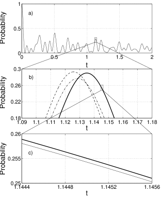
Figure 1: The probability to have zero momentum versus scaled time. a) Overall picture of the probability to have zero momentum. Individual lines are not resolvable at full size. b) The heavy solid line is the full master equation, the dashed line represents the standard adiabatic approximation while the dot-dash line represents the secular approximation. The full master equation is indistinguishable from the more sophisticated adiabatic and dressed state approximations even at this size. c) The thin solid line represents the dressed-state approximation and the sophisticated adiabatic approximation.

Fig. 1b zooms in on a section of the full size figure to illustrate the differences between the approximations. As we can see, the secular and standard adiabatic approximation evolutions both significantly lead that of the full master equation in time. The dressed-state and sophisticated adiabatic approximations are very close to the full master equation solution even at this magnification. Fig 1c zooms in even closer to try to distinguish the sophisticated adiabatic approximation from the full master equation.

This trend continues as we investigate the probability to have 1 atomic unit of momentum in Fig. 2.

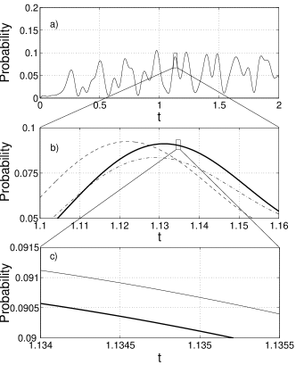
Figure 2: The probability to have 1 atomic unit of momentum versus scaled time. a) Overall picture of the probability to have 1 atomic unit of momentum. Individual lines are again not resolvable at full size. b) The heavy solid line is the full master equation, the dashed line represents the standard adiabatic approximation while the dot-dash line represents the secular approximation. The full master equation is indistinguishable from the more sophisticated adiabatic and dressed state approximations even at this size. c) The thin solid line represents the dressed-state approximation and the sophisticated adiabatic approximation.

The inaccuracy of the secular and standard adiabatic approximations are again evident in Fig. 2b. The more sophisticated adiabatic approximation is very close to the full master equation evolution and is still indistinguishable at this magnification.

Fig. 2c provides a means of comparing the sophisticated adiabatic approximation to the full master equation evolution in detail. As we can see, the more sophisticated adiabatic approximation is again very close to the full master equation.

The last visual comparison to make is to see how the evolution described by the approximations matches that of the full master equation after a very long time period. The time period that has elapsed in Fig. 3 is 8 time units, after which, we would have expected there to be a number of spontaneous emissions. At this point in time, we compare the probability densities described by the approximations and the full master equation.

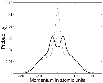
Figure 3: Long time probability density. The solid line represents the full master equation which is indistinguishable from the dressed-state and more sophisticated adiabatic approximations at this magnification. The dashed line represents the standard adiabatic approximation while the dash-dot line is the evolution described by the secular approximation. It is worth noting here that due to our approximations, the probability density is only defined for integer values of momentum. We have “connected the dots”to aid the eye.

It is evident from Fig. 3 that the standard adiabatic and the secular approximations are quite poor methods for simulating the full master equation evolution over a long time period. The main reason for this is the leading behaviour such as we see in Fig. 1a. Even at long times, the probability to have zero momentum is still oscillating and the leading behaviour means that the standard adiabatic and secular approximations are not oscillating in phase with the full master equation. Thus, even though they follow roughly the same shape, they are not necessarily at the same point in the oscillation as the full master equation. What is even more striking though is that the secular approximation evolution seems to follow a slightly different trend for the probabilities to have larger momentum. The intriguing features of the secular approximation are discussed in Sec VIII.

To examine how close the sophisticated adiabatic and the dressed-state approximations are to the full master equation, Fig. 4 focuses on a smaller section to provide a comparison.

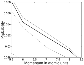
Figure 4: Long time probability density. The heavy solid line represents the full master equation evolution while the thin solid line represents the sophisticated adiabatic and dressed-state approximations. Again the secular and standard adiabatic approximations are represented by the dot dash line and the dashed line respectively.

It is evident from Fig. 4 that the dressed-state and sophisticated adiabatic approximations are very close to the full master equation, even at this long time.

VII.2 Resources

The main resource required to perform the simulations is time. Although each approximation has different memory and processing power requirements, these needs are reasonably accurately reflected in the time each simulation takes to run. The times quoted in table 1 are the times required to calculate the set of results from 0 to 8 time units and are quoted in seconds.

Table 1: Comparison of the times each simulation requires to run.

Simulation	Time (s)
Full Master equation	617.7
Standard Adiabatic Approximation	16.98
More Sophisticated Adiabatic Approximation	18.31
Secular Approximation	76.43
Dressed State Approximation	18.31

As we can see from the results in table 1, the adiabatic approximations are both clearly the fastest. The secular approximation is just over 4 times larger than the adiabatic approximations. This is not entirely unexpected. We would have expected at least a doubling in time by using the methods that included state information. The secular approximation is supposed to force the coherences to zero. Unfortunately, using our method to simulate this allows zero to be anywhere up to $10^{-5}$. This, although small, still has to be processed explaining the four-fold increase in time. One reason it is just over 4 times the time required for the adiabatic approximations could be that after the evolution has been calculated, there is still a partial trace to be performed to obtain a solution of the same form as the adiabatic approximations. We could have limited this time by simulating two coupled equations instead of a full master equation and then would probably have only doubled the time taken.

VIII Discussion

The standard and more sophisticated adiabatic approximations take similar times to simulate, and are much faster than the full master equation. The only difference between them is an extra potential term. It turns out, though, that this Hamiltonian term is quite important in accurately describing the motion of the atom. While the standard approach evolves too quickly and leads that of the full master equation evolution, the more sophisticated approach with the modified potential does not suffer this problem. The evolution described by this more sophisticated approach is very close to the full master equation, even at long times. Of course the dressed-state approximation offers the same accuracy as the sophisticated adiabatic approximation which may be useful if we wanted to simulate an initially excited atom.

These successes contrast the results from the secular approximation. As one can see from Figs. 1 and 2, the secular approximation not only leads the full master equation solution but it also predicts a lower probability to have either zero or one atomic unit of momentum. This result is surprising because the secular approximation master equation is quite similar to the others. Investigating this further, we find that the secular approximation master equation simulation shows that the probability to have 25 atomic units of momentum increases exponentially much faster than any of the other approximations. To analyse this in another manner, we find that for the secular approximation Tr$[\rho]$ falls off from 1 exponentially much faster than any of the other approximations or the full master equation.

If we consider the dressed-state approximation master equation, Eq. (46), we notice that the Hamiltonian terms are, to leading order, the same as the final secular approximation master equation Eq. (30). The only advantage the dressed state approximation has in terms of it’s Hamiltonian is the presence of the higher order term. The leading order Lindbladian terms are also identical with only the higher order terms differing. The dressed-state master equation includes Lindbladian terms which give rise to a momentum kick to the atom (from the $\mathcal{B}$ superoperator) without a change in the internal state of the atom. The higher order secular approximation master equation Lindbladian term provides the opposite. Here there is an internal state change without a momentum kick to the atom. Thus it is quite unexpected that the secular approximation solution should differ so greatly from the dressed-state approximation solution as they are identical in the leading order terms.

It is a fairly simple matter to investigate the effect of the differences between the two approximations by simulating only parts of the master equations. If we only included the Hamiltonian terms from each master equation, the difference would only be the higher order term in the dressed state master equation. This term has the same effect here as it does for the sophisticated adiabatic approximation, correcting the leading behaviour. It does not however account for the secular approximation predicting lower probabilities as it does in Figs. 1 and 2. Thus to investigate the difference between the higher order Lindbladian terms, we drop the $\mathcal{B}$ superoperator from the dressed-state master equation and add it to the secular approximation master equation. This does not correct the problems with the secular approximation nor does it severely affect the dressed-state approximation. This only leaves the inherent difference that the dressed-state master equation provides a correction term without requiring a state change where the secular approximation forces a state change in it’s correction term. Thus we have to conclude that the best approximation to the full master equation involves a Lindbladian term that does not change the internal state of the atom. Lacking it, the secular approximation is the poorest.

One other point to note in this discussion is one of the conditions on which the adiabatic elimination techniques are based. This is that $\Gamma\rho_{ee}$ be much larger than $\mathcal{K}\rho_{ee}$. This will be satisfied if

$$\mathrm{Tr}\left[\rho_{ee}\frac{p_{x}^{2}}{2m}\right]/\Gamma\mathrm{Tr}\left[\rho_{ee}\right]\ll 1.$$ (50)

For the parameter regime of this investigation, it is not obvious that this holds. Fig 5 shows how the ratio in Eq. (50) evolves through time for the sophisticated adiabatic approximation.

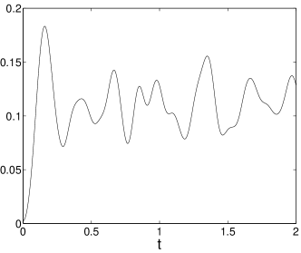
Figure 5: Ratio of Tr$[\rho_{ee}{p_{x}^{2}}/{2m}]$ to Tr$[\Gamma\rho_{ee}]$ for the sophisticated adiabatic approximation. All other simulations look similar.

Here we see that numerically, this ratio is around 0.1 which is of the same order as the other ratios (such as $\Omega_{\rm max}/\delta$) which are required to be small for our approximations.

Finally, we discuss the possibility of simulating with the true experimental parameters. This is difficult because of the stiffness of the full master equation, and the basis size required for all methods. The latter problem can be avoided by using quantum trajectories MolCasDal93 ; DumZolRit92 ; Car93 . Hensinger et al Hen01a actually use quantum trajectory simulations based on the secular approximation master equation. It is however, possible to convert any master equation of the Lindblad form to a quantum trajectory simulation Wiseman . All of the approximate master equations we have developed here have been written in the Lindblad form and as such all of these could be simulated using quantum trajectories.

IX conclusion

There are a number of theoretical models for the motion of an atom as it interacts with a light field. This paper has investigated the possibility of using four different approximations as opposed to using the full master equation to simulate an experimental system. Two have been widely used in the past and two have not. We have given a detailed explanation of the mathematical principles to perform each of these approximations on a fairly general system. We have also compared them numerically to to the true dynamics from the full master equation.

In a regime of particular experimental interest, we have found that the most accurate results are obtained from two approaches that we have introduced here, a sophisticated adiabatic approach and a dressed-state approach. These give identical equations in the regime of interest, and in terms of resources, they are almost as fast to simulate as the standard adiabatic approximation. This has been most used in the past, but deviates significantly from the true dynamics for long times. The other approximation that has been used in the past, the secular approximation, is even poorer. On top of the failings of the standard adiabatic approximation, it takes longer to simulate and appears to produce anomalous momentum diffusion.

- (1) D.A. Steck, W.H. Oskay and M.G. Raizen, Science 293, 274 (2001).
- (2) D.L. Haycock, P.M. Alsing, I.H. Deutsch, J. Grondalski and P.S. Jessen, Phys Rev Let. 85 3365 (2000).
- (3) W.K. Hensinger, A.G. Truscott, B. Upcroft, M. Hug, H.M. Wiseman, N.R. Heckenberg and H. Rubinsztein-Dunlop, Phys Rev A. 64, 033407 (2001).
- (4) W.K. Hensinger, H. Häffner, A. Browaeys, N.R. Heckenberg, K. Helmerson, C. McKenzie, G.J. Milburn, W.D. Phillips, S.L. Rolston, H. Rubinsztein-Dunlop and B. Upcroft, Nature, 412, 52 (2001).
- (5) T. Pellizzari, S.A. Gardiner, J.I. Cirac and P. Zoller, Phys Rev Let. 75, 3788 (1995)
- (6) J.I. Cirac, P. Zoller, H.J. Kimble and H. Mabuchi, Phys Rev Let. 78, 3221 (1997)
- (7) G. Lindblad, Commun. Math. Phys. 48, 199 (1976).
- (8) A.S. Parkins, R. Müller, J. Mod. Opt. 43, 2553, (1996)
- (9) R. Graham, M. Schlautmann and P. Zoller, Phys. Rev. A 45, R19 (1992).
- (10) S. Dyrting and G.J. Milburn, Phys Rev A. 49, 4180 (1994).
- (11) R. Deutschmann, W. Ertmer, and H. Wallis, Phys. Rev. A 47, 2169 (1993).
- (12) J. Dalibard and C. Cohen-Tannoudji, J. Opt. Soc. Am. B, 2, 1707 (1985).
- (13) P. Meystre and M. Sargent III, Elements of Quantum Optics: Third Edition (Springer Verlag, Germany, 1999).
- (14) S.M. Barnett and P.M. Radmore, Methods in Theoretical Quantum Optics (Oxford University Press, United States of America, 1997).
- (15) P. Warszawski and H.M. Wiseman, Phys Rev A. 63, 013803 (2000)
- (16) S.M. Tan, J. Opt. B, 1, 424 (1999).
- (17) S.M. Tan, Quantum Optics Toolbox and accompanying User Guide, http://www.phy.auckland.ac.nz/Staff/ smt/qotoolbox/download.html.
- (18) W.H. Press, B.P. Flannery, S.A. Teukolsky and W.T. Vetterling, Numerical Recipes : The Art of Scientific Computing (Cambridge University Press, United States of America, 1986).
- (19) K. Mølmer, Y. Castin, and J. Dalibard, J. Opt. Soc. Am. B 10, 524 (1993).
- (20) R. Dum, P. Zoller and H. Ritsch, Phys. Rev. A 45, 4879 (1992).
- (21) H.J. Carmichael, An Open Systems Approach to Quantum Optics (Springer-Verlag, Berlin, 1993).
- (22) H. M. Wiseman, Quantum Semiclass. Opt 8, 205 (1996).