Polarization-squeezed light formation in a medium with electronic Kerr nonlinearity

Abstract

We analyze the formation of polarization-squeezed light in a medium with electronic Kerr nonlinearity. Quantum Stokes parameters are considered and the spectra of their quantum fluctuations are investigated. It is established that the frequency at which the suppression of quantum fluctuations is the greatest can be controlled by adjusting the linear phase difference between pulses. We shown that by varying the intensity or the nonlinear phase shift per photon for one pulse, one can effectively control the suppression of quantum fluctuations of the quantum Stokes parameters.
PACS: 42.50.Dv, 42.50.Lc.

Keywords: ultrashort light pulse, self- and cross-phase modulation, electronic Kerr nonlinearity, quantum Stokes parameters.

I Introduction

Knowledge of the quantum properties of the polarization of light is essential when treating issues concerning Einstein-Podolski-Rosen (EPR) paradox [1] or Bell’s inequality [2]. The quantum analysis of the light polarization is generally based on Stokes parameters associated with Hermitian Stokes operators [3, 4]. We call a quantum state to be a polarization-squeezed (PS) state if it has the level of quantum fluctuations of one of the quantum Stokes parameters smaller than the level corresponding to the coherent state [5]. Such a state can be generated by using the optical parametric amplification ($\chi^{2}$) [6, 7]. Recently, effective methods of PS state formation using Kerr-like media ($\chi^{3}$) and optical solitons in fibers have been proposed [5, 8, 9, 10, 11]. In the Kerr medium the self-phase modulation (SPM) occurs, leading to quadrature squeezing with preservation of the photon statistics [12].

It was noted in [13] that a quantum treatment of SPM of ultrashort light pulses (USPs) must account for the additional noise related to the nonlinear absorbtion. The study of the nonlinear propagation in Raman active media [14] accounts for the quantum and thermal noises as a fluctuating addition to the relaxation nonlinearity in the interaction Hamiltonian. However, if we deal with USPs propagation, for instance through fused-silica fibers, the electronic motion on $\sim 1$ fs time scale contributes with about $80$% to the Kerr effect while Raman oscillators give only $20$% contribution [15]. An attempt to develop the quantum theory of pulse SPM has been undertaken in [16], where the electronic Kerr nonlinearity is modelled as a Raman-like one. The electronic nonlinearity was considered correctly with the interaction Hamiltonian [17] and the momentum operator [18] in the normally ordered form.

If two-mode radiation with orthogonal polarization and/or different frequencies propagates through a Kerr medium, then the cross-phase modulation (XPM) and parametric interaction can also occur. The approach in [17, 18] has been extended for the combined SPM–XPM of USPs in [19], by considering the spectra of fluctuations of quadratures. Notice that, for interacting solitons in a Kerr medium with anomalous dispersion ($k^{{}^{\prime\prime}}<0$), the XPM induces the transient photon-number correlations while SPM answers for the intrapulse ones [20].

The experimental realization of the polarization squeezing implies the spatial overlapping of an orthogonally polarized strong coherent beam with squeezed vacuum on a 50 : 50 beamsplitter [21] or the interference of two independent quadrature-squeezed USPs produced in a fiber Sagnac interferometer [8]. The last series of experiments [10, 11] involve both the temporal and spatial overlaps of two orthogonally polarized quadrature-squeezed USPs. From the theoretical point of view, the quantum fluctuations of Stokes parameters in the case of the nonlinear propagation in an isotropic Kerr medium were introduced by the study of the light polarization [4]. The time-independent quantum treatment of two-mode interaction [5] predicted the possibility of forming the PS state in anisotropic Kerr media.

In this letter we report on the theoretical computation of the spectra of fluctuations of the Stokes parameters in the case of two orthogonally polarized propagating USPs in an anisotropic electronic Kerr medium. We employ simultaneously the SPM for quadrature squeezing and the XPM for the PS state formation and its control. The estimations are done in the frame of the quantum theory for SPM-XPM of USPs developed in [19]. The response time of the electronic Kerr nonlinearity is accounted and the dispersion of linear properties is described in the first approximation of the dispersion theory. We begin with a brief description of the model introduced in [19] and based on the momentum operators for the pulse fields. For consistency, we present some elements of the algebra of time-dependent Bose operators. By using such algebra we get the average values, the correlation functions, and the spectra of quantum fluctuations of Stokes parameters. Our concluding remarks close the paper.

II Quantum theory of combined SPM-XPM effect in electronic Kerr medium

The quantum theory developed in [19] is based on the following momentum operators:

$$\hat{G}^{(j)}_{\rm{spm}}(z) = \hbar\beta_{j}\int_{-\infty}^{\infty}dt\int_{-\infty}^{t}H(t-t_{1})\hat{\mathbf{N}}\bigl{[}\hat{n}_{j}(t,z)\hat{n}_{j}(t_{1},z)\bigl{]}dt_{1},$$ (1)

$$\hat{G}_{\rm{xpm}}(z) = \hbar\tilde{\beta}\int_{-\infty}^{\infty}dt\int_{-\infty}^{t}H(t-t_{1})\bigl{[}\hat{n}_{1}(t,z)\hat{n}_{2}(t_{1},z)+\hat{n}_{1}(t_{1},z)\hat{n}_{2}(t,z)\bigl{]}\,dt_{1},$$ (2)

where $j$ is the pulse number, $\beta_{j}$ and $\tilde{\beta}$ are nonlinear coefficients ($\beta_{j}=\hbar\omega_{0}k_{0}n_{2(j)}/8n_{0}V$ [19, 22]) ($j=1,2$), $\hat{\mathbf{N}}$ is the normal ordering operator, $H(t)$ is the nonlinear response function [$H(t)\neq 0$ at $t\geq 0$ and $H(t)=0$ at $t<0$], $\hat{n}_{j}(t,z)=\hat{A}^{+}_{j}(t,z)\hat{A}_{j}(t,z)$ is the “photon number density” operator in the cross-section $z$ of the medium, and $\hat{A}_{j}(t,z)$ and $\hat{A}^{+}_{j}(t,z)$ are the photon anihilation and creation Bose operators with the commutation relations $[\hat{A}_{j}(t_{1},z),\hat{A}^{+}_{k}(t_{2},z)]=\delta_{jk}\delta{(t_{2}-t_{1})}$. The thermal noise is neglected and the expressions (1) and (2) are averaged over the thermal fluctuations. We assume that the Kerr effect is produced by the electronic motion with characteristic time $\tau_{r}\leq 1$ fs. In our approach the pulse duration $\tau_{p}$ is much greater than the relaxation time $\tau_{r}$, and the Kerr medium is lossless and dispersionless; that is, the pulses frequencies are off resonance.

In general, the induced third-order polarization $P^{(3)}$ of the medium at the frequency $\omega$ is: $P^{(3)}_{i}(\omega)=\sum_{j}[\chi^{(3)}_{1122}E_{i}(\omega)E_{j}(\omega)E^{*}_{j}(\omega)+\chi^{(3)}_{1212}E_{j}(\omega)E_{i}(\omega)E^{*}_{j}(\omega)+\chi^{(3)}_{1221}E_{j}(\omega)E_{j}(\omega)E^{*}_{i}(\omega)]$ [5, 23]. Since the first two terms in $P^{(3)}$ involve operator products accounted in (1) and (2), the last term introduces products of the form $\hat{A}^{+^{2}}_{1}\hat{A}^{{}^{2}}_{2}+\hat{A}^{+^{2}}_{2}\hat{A}^{{}^{2}}_{1}$ which are neglected since they are connected with the parametrical interaction. The conditions (also assumed here) under which such terms can be neglected were discussed in [5], where it was noted that the parametric interaction can be neglected if $\Delta z\gg 1$ and the phase mismatch $\Delta=2(k_{2}-k_{1})$ is large, namely $|\Delta|>\rm{min}\{\tilde{\beta}|A_{1}(0)|,\tilde{\beta}|A_{2}(0)|\}$. Here $\tilde{\beta}=8\pi\omega^{2}(\chi^{(3)}_{1122}+\chi^{(3)}_{1212}+\chi^{(3)}_{1221})/c^{2}(k_{1}+k_{2})$, and $k_{j}=(\omega/c)n_{j}$. Note that for circularly polarized modes the last term in $P^{(3)}$ is absent, which is valid in isotropic Kerr media where modes obey only SPM and XPM. For elliptically polarized fields the last term in $P^{(3)}$ induces the circular birefringence $\Delta n_{c}=-(2\pi/n_{0})2\chi^{(3)}_{1221}(|E_{+}(\omega)|^{2}-|E_{-}(\omega)|^{2})$ [23]. However, for the successful experimental overlapping of the two quadrature-squeezed USPs a birefringence compensator is required [10, 11]. In general, $\Delta n_{c}$ can be neglected when USPs propagate along some symmetry directions [23].

Since in our case the Kerr effect is of an electronic origin, in the absence of one- and two-photon and Raman resonances, $H(t)$ can be chosen as $H(t)=(1/\tau_{r})\exp{\left(-t/\tau_{r}\right)}$ at $t\geq 0$ [22]. Then with (1) and (2) the space-evolution equation for $\hat{A}_{1}(t,z)$ in the moving coordinate system ($z=z^{{}^{\prime}}$, $t=t^{{}^{\prime}}-z/u$, where $t^{{}^{\prime}}$ is the running time and $u$ is the group velocity),

$$\frac{\partial\hat{A}_{1}(t,z)}{\partial z}-\bigl{[}\hat{O}_{1}(t)+\hat{\tilde{O}}_{2}(t)\bigl{]}\hat{A}_{1}(t,z)=0,$$ (3)

has the solution given by

$$\hat{A}_{1}(t,z)=e^{\hat{O}_{1}(t)+\hat{\tilde{O}}_{2}(t)}\,\hat{A}_{0,1}(t).$$ (4)

Here $\hat{O}_{j}(t)=i\gamma_{j}q[\hat{n}_{0,j}(t)]$, $\hat{\tilde{O}}_{j}(t)=i\tilde{\gamma}q[\hat{n}_{0,j}(t)]$, $\gamma_{j}=\beta_{j}z$, $\tilde{\gamma}=\tilde{\beta}z$, $\hat{n}_{0,j}(t)=\hat{A}^{+}_{0,j}(t)\hat{A}_{0,j}(t)$ is the “photon number density” operator at the entrance into the medium $z=0$, and $q[\hat{n}_{0,j}(t)]=\int_{-\infty}^{\infty}h(t_{1})\hat{n}_{0,j}(t-t_{1})dt_{1}$, where $h(t)=H(|t|)$. $\hat{A}_{2}(t,z)$ can be derived by changing the indexes $1\leftrightarrow 2$ in (4). In comparison with the so-called nonlinear Schrödinger equation, used in the quantum theory of optical solitons (see [20] and refs. therein), in (3) the pulse dispersion spreading in the medium is absent. This approach corresponds to the first approximation of the dispersion theory [22]. Note that the structure of $q[\hat{n}_{0,j}(t)]$ is like that of the linear response in the quantum description of a USP spreading in the second-order approximation.

The statistical features of pulses at the output of the medium can be evaluated by using the algebra of time-dependent Bose operators [17, 18, 19]. In such algebra we have

$$\hat{A}_{0,j}(t_{1})e^{\hat{O}_{j}(t_{2})}=e^{\hat{O}_{j}(t_{2})+{\mathcal{D}}_{j}(t_{2}-t_{1})}\hat{A}_{0,j}(t_{1}),\quad\hat{A}_{0,j}(t_{1})e^{\hat{\tilde{O}}_{j}(t_{2})}=e^{\hat{\tilde{O}}_{j}(t_{2})+{\tilde{\mathcal{D}}}(t_{2}-t_{1})}\hat{A}_{0,j}(t_{1}),$$ (5)

where ${\mathcal{D}}_{j}(t_{2}-t_{1})=i\gamma_{j}\,h(t_{2}-t_{1})$, ${\tilde{\mathcal{D}}}(t_{2}-t_{1})=i\tilde{\gamma}h(t_{2}-t_{1})$, $2\gamma_{j}$ is the nonlinear phase shift per photon for the $j$-th pulse, and $\tilde{\gamma}$ is the nonlinear coupling coefficient. By using the theorem of normal ordering [17, 18], one obtains the average values of the Bose operators over the initial coherent summary state $|\alpha_{0}(t)\rangle=|\alpha_{0,1}(t)\rangle\otimes|\alpha_{0,2}(t)\rangle$:

$$\langle e^{\hat{O}_{j}(t)}\rangle = e^{i\phi_{j}(t)-\mu_{j}(t)},\quad~{}\langle e^{\hat{\tilde{O}}_{j}(t)}\rangle=e^{i\tilde{\phi}_{j}(t)-\tilde{\mu}_{j}(t)},$$ (6)

$$\langle e^{\hat{O}_{j}(t_{1})+\hat{O}_{j}(t_{2})}\rangle = e^{i[\phi_{j}(t_{1})+\phi_{j}(t_{2})]-[\mu_{j}(t_{1})+\mu_{j}(t_{2})]-{\mathcal{K}}_{j}(t_{1},t_{2})},$$ (7)

$$\langle e^{\hat{\tilde{O}}_{j}(t_{1})+\hat{\tilde{O}}_{j}(t_{2})}\rangle = e^{i[\tilde{\phi}_{j}(t_{1})+\tilde{\phi}_{j}(t_{2})]-[\tilde{\mu}_{j}(t_{1})+\tilde{\mu}_{j}(t_{2})]-\tilde{\mathcal{K}}_{j}(t_{1},t_{2})}.$$ (8)

The parameters $\phi_{j}(t)=2\gamma_{j}\bar{n}_{0,j}(t)$, $\mu_{j}(t)=\gamma^{2}_{j}\bar{n}_{0,j}(t)/2$ are connected with SPM of the $j$-th pulse and $\tilde{\phi}_{j}(t)=2\tilde{\gamma}\bar{n}_{0,j}(t)$, $\tilde{\mu}_{j}(t)=\tilde{\gamma}^{2}\bar{n}_{0,j}(t)/2$ with the pulses’ XPM. Here $\phi_{j}(t)$ ($\tilde{\phi}_{j}(t)$) is the nonlinear phase addition caused by SPM (XPM). The eigenvalue $\alpha_{0,j}(t)$ of the annihilation operator $\hat{A}_{0,j}(t)$ over the coherent state $|\alpha_{0,j}(t)\rangle$ can be written as $\alpha_{0,j}(t)=|\alpha_{0,j}(t)|e^{i\varphi_{j}(t)}$, where $\varphi_{j}(t)$ is the linear phase of the $j$-th pulse. Then $|\alpha_{0,j}(t)|^{2}=\langle\hat{n}_{0,j}(t)\rangle\equiv\bar{n}_{0,j}(t)$. For simplicity let $\bar{n}_{0,j}(t=0)\equiv\bar{n}_{0,j}$. We separate the time dependence in $|\alpha_{0,j}(t)|$ by introducing the pulse’s envelope $r_{j}(t)$ so that $|\alpha_{0,j}(t)|=|\alpha_{0,j}(0)|r_{j}(t)$ with $r_{j}(0)=1$. In (7)-(8), ${\mathcal{K}}_{j}(t_{1},t_{2})=\mu_{0,j}\,r^{2}_{j}(t_{1}+\tau/2)g(\tau)$ and $\tilde{\mathcal{K}}_{j}(t_{1},t_{2})=\tilde{\mu}_{0,j}\,r^{2}_{j}(t_{1}+\tau/2)g(\tau)$ are the temporal correlators, where $\mu_{0,j}=\gamma_{j}\bar{n}_{0,j}$, $\tilde{\mu}_{0,j}=\tilde{\gamma}\bar{n}_{0,j}$, $g(\tau)=(1+|\tau|/\tau_{r})h(\tau)$, and $\tau=t_{2}-t_{1}$.

III Quantum Stokes parameters and their average values, polarization degree

In classical optics the polarization state is visualized as a Stokes vector on the Poincaré sphere and is characterized by the four classical Stokes parameters $\{S_{k}\}_{k=0,3}$. Since $S_{0}$ defines the total intensity of pulse field, $\{S_{k}\}_{k=1,3}$ characterize light polarization and form a Cartesian axis system. Each point on the sphere corresponds to a definite polarization state, whose variation is characterized by the motion of the point on the sphere. In quantum optics, $\{S_{k}\}_{k=0,3}$ are replaced by the operators $\{\hat{S}_{k}\}_{k=0,3}$ which obey: $[\hat{S}_{0},\hat{S}_{i}]=0$, $[\hat{S}_{i},\hat{S}_{j}]=2i\varepsilon_{ijk}\hat{S}_{k}$. We define the quantum Stokes parameters as: $\hat{S}_{0}(t,z)=\sum^{2}_{j=1}\hat{n}_{j}(t,z)$, $\hat{S}_{1}(t,z)=\hat{n}_{1}(t,z)-\hat{n}_{2}(t,z)$,

$$\hat{S}_{2}(t,z) = \hat{A}^{+}_{2}(t,z)\hat{A}_{1}(t,z)+\hat{A}^{+}_{1}(t,z)\hat{A}_{2}(t,z),$$ (9)

$$\hat{S}_{3}(t,z) = i~{}[\hat{A}^{+}_{2}(t,z)\hat{A}_{1}(t,z)-\hat{A}^{+}_{1}(t,z)\hat{A}_{2}(t,z)],$$ (10)

where in our case $\hat{A}_{j}(t,z)$ is given by (4) and $\hat{A}^{+}_{j}(t,z)$ is its Hermitian conjugate. By using Eqs. (5)-(6) we compute the average values of $\{\hat{S}_{k}(t,z)\}_{k=0,3}$ on the coherent summary state $|\alpha_{0}(t)\rangle$. Finally, we get: $\langle\hat{S}_{0}(t,z)\rangle=\sum^{2}_{j=1}\bar{n}_{0,j}(t)$, $\langle\hat{S}_{1}(t,z)\rangle=\bar{n}_{0,1}(t)-\bar{n}_{0,2}(t)$, and

$$\langle\hat{S}_{2}(t,z)\rangle = 2{[\bar{n}_{0,1}(t)\bar{n}_{0,2}(t)]}^{1/2}e^{-[\Delta_{1}(t)+\Delta_{2}(t)]}\cos{[\tilde{\Phi}_{2}(t)-\tilde{\Phi}_{1}(t)]},$$ (11)

$$\langle\hat{S}_{3}(t,z)\rangle = 2{[\bar{n}_{0,1}(t)\bar{n}_{0,2}(t)]}^{1/2}e^{-[\Delta_{1}(t)+\Delta_{2}(t)]}\sin{[\tilde{\Phi}_{2}(t)-\tilde{\Phi}_{1}(t)]},$$ (12)

where $\Delta_{j}(t)=\mu_{j}(t)+\tilde{\mu}_{j}(t)$, $\tilde{\Phi}_{j}(t)=\phi_{j}(t)-\tilde{\phi}_{j}(t)+\varphi_{j}(t)$. By measurements, one obtains a set of measurable quantities associated with the operators (9) and (10). However, the presence of quantum fluctuations results in an uncertainty for the measured quantities. The fluctuation uncertainty of each $\langle\hat{S}_{k}(t,z)\rangle$ can be associated with a particular region of uncertainty on the Poincaré sphere. In the case of the nonlinear propagation, the ball-region of uncertainty, specifically for the coherent state of light, changes to the ellipsoid of uncertainty [5].

In classical optics the polarization degree ${\mathcal{P}}$ is the ratio of the intensity of the polarized part of the radiation $I_{\text{pol}}$ to the total intensity $I_{\text{tot}}$, and is connected with the classical Stokes parameters by ${\mathcal{P}}={\mathcal{R}}/\langle S_{0}\rangle$, where ${\mathcal{R}}$ is the radius of the classical Poincaré sphere, ${\mathcal{R}}^{2}=\sum_{k=1}^{3}\langle S_{k}\rangle^{2}$. Since for completely polarized light ${\mathcal{P}}=1$, for partially polarized light $0<{\mathcal{P}}<1$. The definition of the quantum polarization degree follows the classical one: ${\mathcal{P}}(t,z)={{\mathcal{R}}(t,z)}/\langle\hat{S}_{0}(t,z)\rangle$, where ${\mathcal{R}}^{2}(t,z)=\sum_{k=1}^{3}\langle\hat{S}_{k}(t,z)\rangle^{2}$. With the expressions (11)-(12) we have

$${\mathcal{P}}(t,z)=\{1-4\bar{n}_{0,1}(t)\bar{n}_{0,2}(t)[\bar{n}_{0,1}(t)+\bar{n}_{0,2}(t)]^{-2}(1-e^{-2[\Delta_{1}(t)+\Delta_{2}(t)]})\}^{1/2}.$$ (13)

Since in real-life situations $\Delta_{1}(t)+\Delta_{2}(t)\ll 1$, we have ${\mathcal{P}}(t,z)\approx 1$. Indeed, a recent study [3, 5] investigated the nonlinear behavior of ${\mathcal{P}}(t,z)$ for the nonclassical states of light and revealed that the deviation of ${\mathcal{P}}(t,z)$ from $1$ is a pure quantum effect. Note that the results (11)-(13) are similar to the ones obtained in [5].

IV Correlation functions and spectra of quantum Stokes parameters

Since the Kerr medium is assumed to be lossless and dispersionless, the operators $\hat{S}_{0}(t,z)$ and $\hat{S}_{1}(t,z)$, as well as their dispersions, are conserved. Therefore, we focus our attention to the quantum fluctuations of $\hat{S}_{2}(t,z)$ and $\hat{S}_{3}(t,z)$ by defining their correlation functions as

$$R_{S_{k}}(t_{1},t_{2})=\left\langle\hat{S}_{k}(t_{1},z)\hat{S}_{k}(t_{2},z)\right\rangle-\left\langle\hat{S}_{k}(t_{1},z)\right\rangle\left\langle\hat{S}_{k}(t_{2},z)\right\rangle\qquad(k=2,3).$$ (14)

The correlation functions (14) can be analytically computed by using Eqs. (5) and (7)-(8). Here we simply write down the result for $R_{S_{2}}(t,t+\tau)$ in the approximation $\gamma_{j},\tilde{\gamma}\ll 1$:

$$R_{S_{2}}(t,t+\tau) = \delta(\tau)+h(\tau)[\bar{n}_{0,1}(t)\phi_{2}(t)-\bar{n}_{0,2}(t)\phi_{1}(t)]\sin{2[\tilde{\Phi}_{1}(t)-\tilde{\Phi}_{2}(t)]}$$ (15)

$$+ g(\tau)\{\bar{n}_{0,1}(t)[\phi^{2}_{2}(t)\!+\!\tilde{\phi}^{2}_{2}(t)]+\bar{n}_{0,2}(t)[\phi^{2}_{1}(t)\!+\!\tilde{\phi}^{2}_{1}(t)]\}\sin^{2}{[\tilde{\Phi}_{1}(t)\!-\!\tilde{\Phi}_{2}(t)]},$$ (16)

where for simplicity we denote $t_{1}=t$, $t_{2}=t+\tau$. In the absence of SPM [$\phi_{j}(t)=0$] and XPM [$\tilde{\phi}_{j}(t)=0$] of pulses, Eq. (16) gives us the correlation function for the coherent state $R_{S_{2}}^{coh}(t,t+\tau)=\delta(\tau)$, as expected. The spectral densities of quantum fluctuations of $\hat{S}_{k}(t,z)$ can be evaluated by using Wiener-Khintchine theorem: $S_{S_{k}}(\omega,t)=\int_{-\infty}^{\infty}R_{S_{k}}(t,t+\tau)e^{i\omega\tau}d\tau$. Allowing for a small change of the envelope during the relaxation time we obtain

$$S_{S_{2}}(\Omega,t) = 1+2L(\Omega)[\bar{n}_{0,1}(t)\phi_{2}(t)-\bar{n}_{0,2}(t)\phi_{1}(t)]\sin{2[\tilde{\Phi}_{1}(t)-\tilde{\Phi}_{2}(t)]}$$ (17)

$$+ 4L^{2}(\Omega)\{\bar{n}_{0,1}(t)[\phi^{2}_{2}(t)\!+\!\tilde{\phi}^{2}_{2}(t)]+\bar{n}_{0,2}(t)[\phi^{2}_{1}(t)\!+\!\tilde{\phi}^{2}_{1}(t)]\}\sin^{2}{[\tilde{\Phi}_{1}(t)\!-\!\tilde{\Phi}_{2}(t)]},$$ (18)

where $L(\Omega)=1/(1+\Omega^{2})$, and $\Omega=\omega\tau_{r}$ is the reduced frequency. The spectral density (18) depends on the relaxation time $\tau_{r}$ and quasi-statically changes with time. Besides, the second term on r.h.s. of Eq. (18) indicates that the quantum fluctuations of $\hat{S}_{2}(t,z)$ can be less than those corresponding to the coherent state $S_{S_{2}}^{coh}(\Omega,t)=1$. The correlation function of $\hat{S}_{3}(t,z)$, as well as its spectrum, can be easily obtained by shifting (16) and (18) in phase with $\pi/2$.

For an arbitrary $\Omega_{0}=\omega_{0}\tau_{r}$, at which the linear phase difference between incoming pulses

$$\Delta\varphi(t)_{\rm opt} = \frac{1}{2}\arctan\left(\frac{\bar{n}_{0,1}(t)\phi_{2}(t)-\bar{n}_{0,2}(t)\phi_{1}(t)}{L(\Omega_{0})\Bigl{\{}\bar{n}_{0,1}(t)[\phi^{2}_{2}(t)+\tilde{\phi}^{2}_{2}(t)]+\bar{n}_{0,2}(t)[\phi^{2}_{1}(t)+\tilde{\phi}^{2}_{1}(t)]\Bigl{\}}}\right)$$ (20)

$$+\phi_{1}(t)-\phi_{2}(t)-\tilde{\phi}_{1}(t)+\tilde{\phi}_{2}(t),$$

is optimized, the expression (18) reaches the minimum value:

$$S_{S_{2}}(\Omega_{0},t) = 1+2L^{2}(\Omega_{0})\{\bar{n}_{0,1}(t)[\phi^{2}_{2}(t)+\tilde{\phi}^{2}_{2}(t)]+\bar{n}_{0,2}(t)[\phi^{2}_{1}(t)+\tilde{\phi}^{2}_{1}(t)]\}$$ (23)

$$-2L(\Omega_{0})\Bigl{(}[\bar{n}_{0,1}(t)\phi_{2}(t)-\bar{n}_{0,2}(t)\phi_{1}(t)]^{2}$$

$$+L^{2}(\Omega_{0})\{\bar{n}_{0,1}(t)[\phi^{2}_{2}(t)+\tilde{\phi}^{2}_{2}(t)]+\bar{n}_{0,2}(t)[\phi^{2}_{1}(t)+\tilde{\phi}^{2}_{1}(t)]\}^{2}\Bigl{)}^{1/2}.$$

To characterize the deviation of $S_{S_{2}}(\Omega,t)$ from the coherent level, we define the normalized spectral variance $S^{*}_{S_{2}}(\Omega,t)=[S_{S_{2}}(\Omega,t)-1]/\bar{n}_{0,1}(t)$. In the case of the suppression of quantum fluctuations $-1\leq S^{*}_{S_{2}}(\Omega,t)<0$. Let us investigate the $S^{*}_{S_{2}}(\Omega,t)$ by choosing the linear phase difference between pulses to be optimal at a defined reduced frequency $\Omega_{0}$, and change the intensity of one pulse (the control pulse) in comparison with the intensity of the other one. Such dependence of $S^{*}_{S_{2}}(\Omega,t)$ at $t=0$ and $\Omega=0$ on the maximum nonlinear phase addition $\phi_{0,1}\equiv\phi_{1}(t=0)$ in case the linear phase difference is optimal at $\Omega_{0}=0$ and $\Omega_{0}=1$, is displayed in Figs. 1 and 2, respectively.

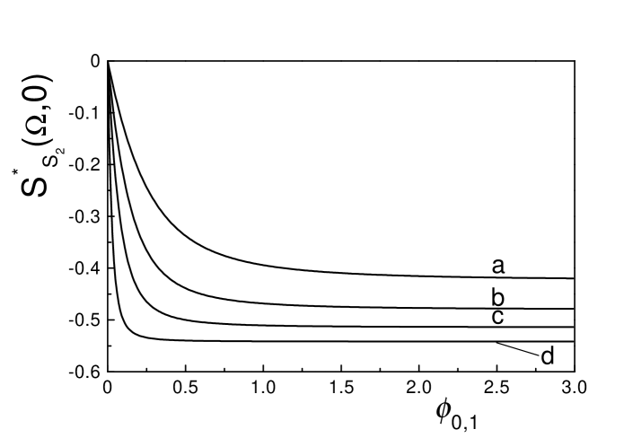
FIG. 1.: Normalized spectral variance $S^{*}_{S_{2}}(\Omega,t)$ as a function of the maximum nonlinear phase addition $\phi_{0,1}$ at the reduced frequency $\Omega=0$ for initial phase difference $\Delta\varphi(t)$ which is optimal at $\Omega_{0}=0$. Curves are calculated at time $t=0$, $\gamma_{1}=\gamma_{2}/4=2\tilde{\gamma}$, and correspond to $\bar{n}_{0,2}=\bar{n}_{0,1}/4$ (a), $\bar{n}_{0,2}=\bar{n}_{0,1}/2$ (b), $\bar{n}_{0,2}=\bar{n}_{0,1}$ (c), $\bar{n}_{0,2}=3\bar{n}_{0,1}$ (d).

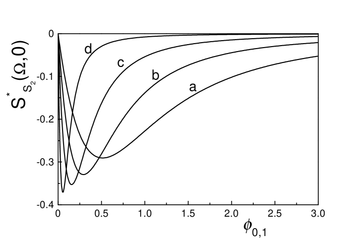
FIG. 2.: As in Fig. 1 but for $\Omega_{0}=1$.

Thus, at $\Omega_{0}=0$ the increase of the control pulse intensity produces a uniform suppression of quantum fluctuation of $\hat{S}_{2}(t,z)$ for any $\phi_{0,1}>1$. At $\Omega_{0}=1$ the increase of the control pulse intensity produces the suppression basically in the domain $\phi_{0,1}<1$. The normalized spectral variance $S^{*}_{S_{2}}(\Omega,t)$ at $t=0$, $\Omega_{0}=0$, and fixed $\phi_{0,1}=2$, is presented in Fig. 3.

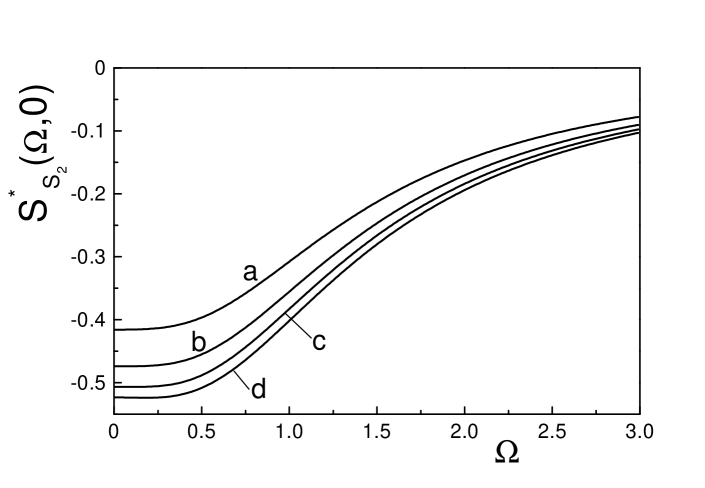
FIG. 3.: Normalized spectral variance $S^{*}_{S_{2}}(\Omega,t)$ at $\phi_{0,1}=2$ for initial phase difference $\Delta\varphi(t)$ which is optimal at $\Omega_{0}=0$. Curves are calculated at time $t=0$, $\gamma_{1}=\gamma_{2}/4=2\tilde{\gamma}$, and correspond to $\bar{n}_{0,2}=\bar{n}_{0,1}/4$ (a), $\bar{n}_{0,2}=\bar{n}_{0,1}/2$ (b), $\bar{n}_{0,2}=\bar{n}_{0,1}$ (c), $\bar{n}_{0,2}=3\bar{n}_{0,1}$ (d).

Now the suppression in $\hat{S}_{2}(t,z)$ is maximal at $\Omega\approx 0$. Summarizing, the choice of the linear phase difference allows us to obtain the spectra with the form of interest, and the increase of the control pulse intensity can effectively control the suppression of quantum fluctuations of quantum Stokes parameters.

One can also control the suppression of quantum fluctuations of $\hat{S}_{2}(t,z)$ by increasing the nonlinear coefficient $\gamma_{2}$ in comparison with $\gamma_{1}$. This is equivalent to the increase of the Kerr electronic nonlinearity for one pulse $n_{2(2)}$ in comparison with the one for another pulse $n_{2(1)}$ ($\gamma_{j}=\beta_{j}z$). The variance $S^{*}_{S_{2}}(\Omega,t)$ at $t=0$, $\Omega_{0}=0$ for various relations between nonlinear coefficients $\gamma_{1}$ and $\gamma_{2}$ is displayed in Fig. 4 in the simplest case of pulses with the same intensity.

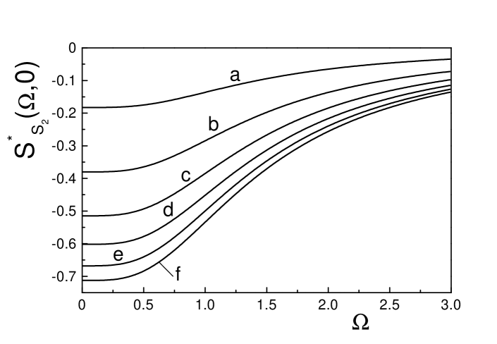
FIG. 4.: Normalized spectral variance $S^{*}_{S_{2}}(\Omega,t)$ at $\phi_{0,1}=2$ for initial phase difference $\Delta\varphi(t)$ which is optimal at $\Omega_{0}=0$. Curves are calculated at time $t=0$, $\bar{n}_{0,1}=\bar{n}_{0,2}$, $\tilde{\gamma}=\gamma_{1}/2$ and correspond to $\gamma_{2}=2\gamma_{1}$ (a), $\gamma_{2}=3\gamma_{1}$ (b), $\gamma_{2}=4\gamma_{1}$ (c), $\gamma_{2}=5\gamma_{1}$ (d), $\gamma_{2}=6\gamma_{1}$ (e), $\gamma_{2}=7\gamma_{1}$ (f).

In this case, the increase of $\gamma_{2}$ in comparison with $\gamma_{1}$ suppresses the quantum fluctuations of $\hat{S}_{2}(t,z)$ basically at low frequencies, $\Omega\approx 0$ . A similar dependence, but at $\Omega_{0}=1$, is shown in Fig. 5.

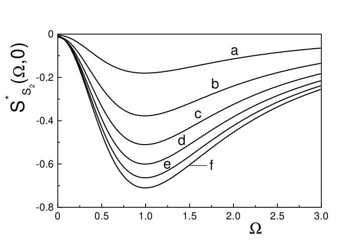
FIG. 5.: As in Fig. 4 but for $\Omega_{0}=1$

Now, the squeezing takes place essentially at $\Omega\approx 1$ ($\omega\approx 1/\tau_{r}$).

Note the experimentally obtained squeezing of $-2.8$ dB in $\hat{S}_{2}$ reported in [10]. The calculations in [10] use quantum noise operators and do not account for the finite relaxation time of the Kerr nonlinearity. However, the relaxation time, which was accounted here, is of a fundamental importance since it determines the level of quantum fluctuations of Stokes operators below the level corresponding to the coherent state [see Eq. (18)]. Besides, we indicated the optimal strategy for the successful generation of the PS state in the electronic Kerr medium.

V Conclusion

We investigated the formation of polarization-squeezed light in a nonlinear medium with electronic Kerr nonlinearity. The correlation functions and corresponding spectra of quantum Stokes parameters $\hat{S}_{2}$ and $\hat{S}_{3}$ were considered. We shown that, by adjusting the linear phase difference between pulses, the maximum suppression of the quantum fluctuations of $\hat{S}_{2}$ or $\hat{S}_{3}$ can be realized at the spectral component of interest. It is established that the increase of the intensity of the control pulse can be employed to suppress the quantum fluctuations of $\hat{S}_{2}$. We find that the increase of one nonlinear coefficient ($\gamma_{2}$) in comparison with another one ($\gamma_{1}$) produces a substantial suppression of quantum fluctuations of $\hat{S}_{2}$.

REFERENCES

[1] Ou Z. Y., Pereira S. F., Kimble H. J., Peng K.
C., Phys. Rev. Lett., 68, 1992 (3663).
[2] Aspect A., Grangier P. Roger G., Phys. Rev.
Lett., 49, 1982 (91).
[3] Agarwal G. S. Puri R. R., Phys. Rev. A, 40, 1989 (5179).
[4] Tanas R. Kielich S., J. Mod. Opt., 37, 1990 (1935).
[5] Chirkin A. S., Orlov A. A., Paraschuk D. Yu.,
Kvant. Elektron., 20, 1993 (999), [Quantum
Electron., 23, 1993 (870)].
[6] Grangier P., Slusher R. E., Yurke B., LaPorta A., Phys. Rev.
Lett., 59, 1987 (2153).
[7] Bowen W. P., Treps N., Schnabel R., Lam P.
K., Phys. Rev. Lett., 89, 2002 (253601).
[8] Silberhorn Ch., Lam P. K., Wei O., König F., Korolkova N. Leuchs
G., Phys. Rev. Lett., 86, 2001 (4267).
[9] Korolkova N. V., Leuchs G., Loudon R., Ralph T. C., Silberhorn
C., Phys. Rev. A, 65, 2002 (052306).
[11] Glöckl O., Heersnik J, Korolkova N. V., Leuchs G., and Lorenz
S., J. Opt. B: Quantum Semiclass. Opt., 5, 2003 (S492).
[12] Kitagawa M. Yamamoto Y., Phys. Rev. A, 34, 1986 (3974).
[13] Blow J. K., Loudon R., Phoenix S. J. D., J. Opt. Soc. Am.
B, 8, 1991 (1750).
[14] Boivin L., Kärtner F. X., Haus A. H., Phys. Rev.
Lett., 73, 1994 (240).
[15] Joneckis L. G. Shapiro J. H., J. Opt. Soc. Am.
B, 10, 1993 (1102).
[16] Boivin L., Phys. Rev. A, 52, 1994 (754).
[17] Popescu F. and Chirkin A. S., Pis’ma Zh. Eksp. Teor. Fiz., 69, 1999 (481),
[JETP Lett., 69, 1999 (516)].
[18] Chirkin A. S. Popescu F., J. Russ. Laser Research, 22, 2001 (354).
[19] Popescu F. Chirkin A. S., J. Opt. B: Quantum Semiclass.
Opt., 4, 2002 (184).
[20] König F., Zielonka M. A., Sizmann A.,
Phys. Rev. A, 66, 2002 (013812).
[21] Hald J., Sørensen J. L., Schori C., Polzik, E. S., J. Mod.
Optics, 47, 2001 (2599).
[22] Akhmanov S. A., Vysloukh V. A., Chirkin A. S., Optics of
Femtosecound Laser Pulses, AIP, New York (1992) [Supplemented translation
of Russian original, Nauka, Moscow (1988)].
[23] Shen Y. R. The Principles of Nonlinear Optics, John
Wiley & Sons, Inc., (1984).