Optimized quantum nondemolition measurement of a field quadrature

Abstract

We suggest an interferometric scheme assisted by squeezing and linear feedback to realize the whole class of field-quadrature quantum nondemolition measurements, from Von Neumann projective measurement to fully non-destructive non-informative one. In our setup, the signal under investigation is mixed with a squeezed probe in an interferometer and, at the output, one of the two modes is revealed through homodyne detection. The second beam is then amplitude-modulated according to the outcome of the measurement, and finally squeezed according to the transmittivity of the interferometer. Using strongly squeezed or anti-squeezed probes respectively, one achieves either a projective measurement, i.e. homodyne statistics arbitrarily close to the intrinsic quadrature distribution of the signal, and conditional outputs approaching the corresponding eigenstates, or fully non-destructive one, characterized by an almost uniform homodyne statistics, and by an output state arbitrarily close to the input signal. By varying the squeezing between these two extremes, or simply by tuning the internal phase-shift of the interferometer, the whole set of intermediate cases can also be obtained. In particular, an optimal quantum nondemolition measurement of quadrature can be achieved, which minimizes the information gain versus state disturbance trade-off.

I Introduction

In order to be manipulated and transmitted information should be encoded into some degree of freedom of a physical system. Ultimately, this means that the input alphabet should correspond to the spectrum of some observable, i.e. that information is transmitted using quantum signals. At the end of the channel, to retrieve this kind of quantum information, one should measure the corresponding observable. As a matter of fact, the measurement process unavoidably introduces some disturbance, and may even destroys the signal, as it happens in many quantum optical detectors, which are mostly based on the irreversible absorption of the measured radiation. Actually, even in a measurement scheme that somehow preserves the signal for further uses, one is faced by the information gain versus state disturbance trade-off, i.e. by the fact that the more information is obtained, the more the signal under investigation is being modified.

Actually, the most informative measurement of an observable $X$ on a state $|\psi\rangle$ corresponds to its ideal projective measurement, which is also referred to as Von Neumann second kind quantum measurement [1]. In an ideal projective measurement the outcome $x$ occurs with the intrinsic probability density $|\langle\psi|x\rangle|^{2}$, whereas the system after the measurement is left in the corresponding eigenstate $|x\rangle$. A projective measurement is obviously repeatable, since a second measure gives the same outcome as the first one. However, the initial state is erased, and the conditional output do not permit to obtain further information about the input signal. The opposite case corresponds to a fully non-destructive detection scheme, where the state after the measurement can be made arbitrarily close to the input signal, and which is characterized by an almost uniform output statistics, i.e. by a data sample that provides almost no information.

Besides fundamental interest, the realization of a projective measurement of the quadrature would have application in quantum communication based on continuous variables. In facts, it provides a reliable and controlled source of optical signals. On the other hand, a fully non-destructive measurement scheme is an example of a quantum repeater, another relevant tool for the realization of quantum network. Between these two extremes we have the entire class of quantum nondemolition (QND) measurements. Such intermediate schemes provide only a partial information about the measured observable, and correspondingly are only partially distorting the signal under investigation. In particular, in this paper, we show how to attain an optimized QND measurement of quadrature i.e. scheme which minimizes the information gain versus state disturbance trade-off.

Most of the schemes suggested for back-action evading measurements are based on nonlinear interaction between signal and probe taking place either in $\chi^{(3)}$ or $\chi^{(3)}$ media (both fibers and crystals) [2, 3, 4, 5, 6, 7, 8], or on optomechanical coupling [9, 10]. A beam-splitter based scheme has been earlier suggested to realize optical Von Neumann measurement [11]. Here, we focus our attention on an interferometric scheme which requires only linear elements and single-mode squeezers.

A schematic diagram of the suggested setup is given in Fig. 1. The signal under examination $|\psi_{\sc s}\rangle$ and the probe (meter) state $|\psi_{\sc p}\rangle$ are given by

$$|\psi_{\sc s}\rangle = \int dx\>\psi_{\sc s}(x)\>|x\rangle_{1}$$ (1)

$$|\psi_{\sc p}\rangle = \int dx\>\psi_{\sc p}(x)\>|x\rangle_{2}\;,$$ (2)

where $|x\rangle_{j}$, $j=1,2$ are eigenstates of the field quadratures $x_{j}=1/2(a_{j}^{\dagger}+a_{j})$, $j=1,2$ of the two modes, and $\psi_{\sc s}(x)$ and $\psi_{\sc p}(x)$ are the corresponding wave-functions. The two beams are linearly mixed in a Mach-Zehnder interferometer with internal phase-shift given by $\phi$. There are also two $\lambda/4$ plates, each imposing a $\pi/2$ phase-shift. Overall, the interferometer equipped with the plates is equivalent to a beam splitter of transmittivity $\tau=\cos^{2}\phi$. However, the interferometric setup is preferable to a single beam splitter since it permits a fine tuning of the transmittivity. After the interferometer, one of the two output modes is revealed by homodyne detection, whereas the second mode is firstly displaced by an amount that depends on the outcome of the measurement (feedback assisted amplitude modulation), and then squeezed according to the transmittivity of the interferometer (see details below). As we will see, either by tuning the phase-shift of the interferometer, or by exciting the probe state $|\psi_{\sc p}\rangle$ in a squeezed vacuum, and by varying the degree of squeezing, the action of the setup ranges from a projective to a non-destructive measurement of the field quadrature as follows:

1. the statistics of the homodyne detector ranges from a distribution arbitrarily close to the intrinsic quadrature probability density of the signal state $|\psi_{\sc s}(x)|^{2}$ to an almost uniform distribution;

2. the conditional output state, after registering a value $x_{0}$ for the quadrature of the signal mode, ranges from a state arbitrarily close to the corresponding quadrature eigenstate $|x_{0}\rangle$ to a state that approaches the input signal $|\psi_{\sc s}\rangle$.

The two features can be summarized by saying that the present scheme realizes the whole set of QND measurements of a field quadrature. In addition, the interferometer can be tuned in order to minimize the information gain versus state disturbance trade-off, i.e. to achieve an optimal QND measurement of quadrature. Such a kind of measurement provides the maximum information about the quadrature distribution of the signal, while keeping the conditional output state as close as possible to the incoming signal.

The paper is structured as follows. In the next Section we analyze the dynamics of the measurement scheme, and describe in details the action of linear feedback and tunable squeezing on the conditional output state and on the homodyne distribution. In Section III we analyze the limiting cases of strongly squeezed and anti-squeezed probes, which correspond to projective and non-destructive measurements respectively. In Section IV we introduce two fidelity measures, in order to quantify how close are the conditional output and the homodyne distribution to the input signal and its quadrature distribution respectively. As a consequence, we are able to individuate an optimal set of configurations that minimize the trade-off between information gain and state disturbance. Section V closes the paper with some concluding remarks.

II Homodyne interferometry with linear feedback

Let us now describe the interaction scheme in details. The evolution operator of the interferometer is given by $U(\phi)=\exp\left[i\phi\left(a_{1}^{\dagger}a_{2}+a^{\dagger}_{2}a_{1}\right)\right]$, such that the input state $|\Psi_{\sc in}\rangle\rangle=|\psi_{\sc s}\rangle\otimes|\psi_{\sc p}\rangle$ evolves as

$$|\Psi_{\sc out}\rangle\rangle = U(\phi)\>|\psi_{\sc s}\rangle\otimes|\psi_{\sc p}\rangle=$$ (3)

$$= \int dx_{1}\int dx_{2}\>\psi_{\sc s}(x_{1})\>\psi_{\sc p}(x_{2})\>|x_{1}\cos\phi+x_{2}\sin\phi\rangle_{1}\otimes|-x_{1}\sin\phi+x_{2}\cos\phi\rangle_{2}$$ (4)

$$= \int dy_{1}\int dy_{2}\>\psi_{\sc s}(y_{1}\cos\phi-y_{2}\sin\phi)\>\psi_{\sc p}(y_{1}\cos\phi+y_{2}\sin\phi)\>|y_{1}\rangle_{1}\otimes|y_{2}\rangle_{2}\;.$$ (5)

After the interferometer the quadrature of one of the modes (say mode $2$) is revealed by homodyne detection. The distribution of the outcomes is given by

$$p(X)=\hbox{Tr}\left[\>|\Psi_{\sc out}\rangle\rangle\langle\langle\Psi_{\sc out}|\>{\mathbb{I}}_{1}\otimes\Pi_{2}(X)\right]\qquad\Pi(X)=|X\rangle\langle X|\;,$$ (6)

$\Pi(x)$ being the POVM of the homodyne detector. Since the reflectivity of the interferometer is given by $\sin\phi$ from an outcome $X$ by the homodyne we infer a value $x_{0}=-X/\sin\phi$ for the quadrature of the input signal. The corresponding probability density is given by

$$p(x_{0})=-\sin\phi\>p(X)=\tan\phi\int dy\>|\psi_{\sc s}(y)|^{2}\>\left|\psi_{\sc p}\left[\tan\phi(y-x_{0})\right]\right|^{2}\;,$$ (7)

and the conditional output state for the mode $1$

$$|\varphi_{x_{0}}\rangle = \sqrt{\sin\phi}\>\langle-X\sin\phi|\Psi_{\sc out}\rangle\rangle=$$ (8)

$$= \sqrt{\frac{\sin\phi}{p(x_{0})}}\int dy\>\psi_{\sc s}(y\cos\phi+x_{0}\sin^{2}\phi)\>\psi_{\sc p}(y\sin\phi-x_{0}\cos\phi\sin\phi)\>|y\rangle\;.$$ (9)

The amplitude of this conditional state is then modulated by a feedback mechanism, which consists in the application of a displacement $D(x_{0}\sin\phi\tan\phi)$, with $D(z)=\exp(za^{\dagger}-\bar{z}a)$. Such displacing action can be obtained by mixing the mode with a strong coherent state of amplitude $z$ (e.g. the laser beam also used as local oscillator for the homodyne detector, see Fig. 1) in a beam splitter of transmittivity $\tau$ close to unit, with the requirement that $z\sqrt{1-\tau}=x_{0}\sin\phi\tan\phi$ [12]. An experimental implementation using a feedforward electro-optic modulator has been presented in [13]. The resulting state is given by

$$D(x_{0}\sin\phi\tan\phi)\>|\varphi_{x_{0}}\rangle=\sqrt{\frac{\sin\phi}{p(x_{0})}}\int dy\>\psi_{\sc s}(y\cos\phi)\>\psi_{\sc p}(y\sin\phi-x_{0}\tan\phi)\>|y\rangle\;.$$ (10)

Finally, this state is subjected to a single-mode squeezing transformation $S(r)=\exp[1/2r(a^{{\dagger}2}-a^{2})]$ by a degenerate parametric amplifier (DOPA). By tuning the squeezing parameter to a value $r^{\star}=\cos\phi$ and using the relation $S(r)|y\rangle=e^{r/2}|e^{r}y\rangle$ we arrive at the final state

$$|\psi_{x_{0}}\rangle = S(r^{\star})\>D(x_{0}\sin\phi\tan\phi)\>|\varphi_{x_{0}}\rangle=$$ (11)

$$= \sqrt{\frac{\tan\phi}{p(x_{0})}}\int dy\>\psi_{\sc s}(y)\>\psi_{\sc p}\left[(y-x_{0})\tan\phi\right]\>|y\rangle\;.$$ (12)

The wave-function of this conditional output state is thus given by

$$\psi_{x_{0}}(x)=\frac{\psi_{\sc s}(x)\>\psi_{\sc p}\left[(x-x_{0})\tan\phi\right]}{\sqrt{\int dy\>|\psi_{\sc s}(y)|^{2}\>\left|\psi_{\sc p}\left[\tan\phi(y-x_{0})\right]\right|^{2}}}\;.$$ (13)

Eq. (7) and Eqs. (12,13) summarize the filtering effects of the probe wave-function on the output statistics and the conditional state respectively.

III Measurements using squeezed or anti-squeezed probes

For the probe mode in the vacuum state we have $\psi_{\sc p}(x)=(2/\pi)^{-1/4}\exp(-x^{2})$ such that the homodyne distribution of Eq. (7) results

$$p(x_{0})=|\psi_{\sc s}(x)|^{2}\star G(x,x_{0},\frac{1}{4\tan^{2}\phi})\;$$ (14)

where $\star$ denotes convolution and $G(x;x_{0},\sigma^{2})$ a Gaussian of mean $x_{0}$ and variance $\sigma^{2}$. The quadrature distribution of the corresponding output state is given by

$$|\psi_{x_{0}}(x)|^{2}=\frac{1}{p(x_{0})}|\>\psi_{\sc s}(x)|^{2}\>G(x,x_{0},\frac{1}{4\tan^{2}\phi})\;$$ (15)

Eqs (14) and (15) account for the noise introduced by vacuum fluctuations. This noise can be manipulated by suitably squeezing the probe, thus realizing the whole set of QND measurement.

Squeezed or anti-squeezed vacuum probes are described by the wave-functions

$$\psi_{\sc sq}(x) = \frac{1}{(2\pi\Sigma^{2})^{1/4}}\exp\left\{-\frac{x^{2}}{4\Sigma^{2}}\right\}$$ (16)

$$\psi_{\sc asq}(x) = \left(\frac{\Sigma^{2}}{2\pi}\right)^{1/4}\exp\left\{-\frac{\Sigma^{2}x^{2}}{4}\right\}\;,$$ (17)

where the information about squeezing stays in the requirement $0<\Sigma^{2}\leq 1/4$. Notice that squeezing the probe introduces additional energy in the system. The mean photon number of the states in (17) is given by $N=(\Sigma^{2}+1/\Sigma^{2}-2)/4$. Using a squeezed vacuum probe Eqs. (14) and (15) rewrites as

$$p(x_{0}) = |\psi_{\sc s}(x)|^{2}\star G(x,x_{0},\Sigma^{2}/\tan^{2}\phi)\stackrel{{\scriptstyle\Sigma\rightarrow 0}}{{\longrightarrow}}|\psi_{\sc s}(x_{0})|^{2}$$ (18)

$$|\psi_{x_{0}}(x)|^{2} = \frac{1}{p(x_{0})}\>|\psi_{\sc s}(x)|^{2}\>G(x,x_{0},\Sigma^{2}/\tan^{2}\phi)\stackrel{{\scriptstyle\Sigma\rightarrow 0}}{{\longrightarrow}}\delta(x-x_{0})\;.$$ (19)

Eq. (18) says that by squeezing the probe the statistics of the homodyne detectors can be made arbitrarily close to the intrinsic quadrature distribution $|\psi_{\sc s}(x_{0})|^{2}$, whereas Eq. (19) shows that, for any value of the outcome $x_{0}$, the conditional output $|\psi_{x_{0}}\rangle$ approaches the corresponding quadrature eigenstate $|x_{0}\rangle$. For $\Sigma\rightarrow 0$ the mean energy of the conditional output state $|\psi_{x_{0}}\rangle$ increases, since it is approaching a quadrature eigenstate (an exact eigenstate would have infinite energy). Notice that this amount of energy is mostly provided by the probe state itself, rather than by the displacement and squeezing stages of the setup. The improvement in the precision due to squeezing, compared to that of a vacuum probe, can be quantified by the ratio of variances in the filtering Gaussian of Eqs. (15) and (19). Calling this ratio $\Delta$ we have $\Delta=\Sigma^{2}$ and thus, for squeezing not too low, $\Delta\simeq N$.

For an anti-squeezed vacuum probe Eqs. (14) and (15) rewrites as

$$p(x_{0}) = |\psi_{\sc s}(x)|^{2}\star G(x,x_{0},(\Sigma^{2}\tan^{2}\phi)^{-1})\stackrel{{\scriptstyle\Sigma\rightarrow 0}}{{\longrightarrow}}\frac{\exp\{-\frac{x^{2}}{2\sigma^{2}}\}}{\sqrt{2\pi\sigma^{2}}}\quad\sigma^{2}=\frac{1}{\Sigma^{2}\tan^{2}\phi}$$ (20)

$$|\psi_{x_{0}}(x)|^{2} = \frac{1}{p(x_{0})}\>|\psi_{\sc s}(x)|^{2}\>G(x,x_{0},(\Sigma^{2}\tan^{2}\phi)^{-1})\stackrel{{\scriptstyle\Sigma\rightarrow 0}}{{\longrightarrow}}|\psi_{\sc s}(x)|^{2}\quad\forall x_{0}\;.$$ (21)

Eqs. (20) and (21) says that by anti-squeezing the probe the statistics of the homodyne detectors is approaching a flat distribution over the real axis, and correspondingly that the conditional output can be made arbitrarily close to the incoming signal, independently on the actual value of $x_{0}$.

Notice that, in principle, both projective and non-destructive measurements could be obtained with vacuum probe, simply by varying the internal phase-shift of the interferometer according to Eqs. (14) and (15). However, this would affect also the rate of the events at the output (since $\phi$ governs the transmittivity of the interferometer), and therefore may be not convenient from practical point of view. On the other hand, when a fine tuning of the variances in Eqs. (18-21) is needed (as for example in the optimization of the scheme, see next Section) it can be conveniently obtained by varying $\phi$, without the need of varying the degree of squeezing of the probe.

IV Optimized QND measurement

So far we considered the two extreme cases of infinitely squeezed or antisqueezed probes. Now we proceed to quanti-fy the trade-off between the state disturbance and the gain of information for the whole set of intermediate cases. There are two relevant parameters: i) how close the output signal is to the input state, and ii) how close the homodyne distribution is to the intrinsic quadrature probability. According to Eq. (12), after the outcome $x$ is being registered the conditional output state is given by $|\psi_{x}\rangle$. Since the outcome $x$ occurs with the probability $p(x)$ of Eq. (7), the density matrix describing the output ensemble after a large number of measurements is given by

$$\varrho_{\sc out}=\int dx\>p(x)\>|\psi_{x}\rangle\langle\psi_{x}|\;.$$ (22)

Indeed, this is the state that can be subsequently manipulated, or used to gain further information on the system. The resemblance between input and output can be quantified by the average state fidelity

$$F=\langle\psi_{\sc s}|\varrho_{\sc out}|\psi_{\sc s}\rangle=\int dx\>p(x)\>\left|\langle\psi_{\sc s}|\psi_{x}\rangle\right|^{2}\;.$$ (23)

Inserting Eq. (12) in Eq. (23) we obtain

$$F=\int\int dy^{\prime}dy^{\prime\prime}\>\left|\psi_{\sc s}(y^{\prime})\right|^{2}\>\left|\psi_{\sc p}(y^{\prime\prime})\right|^{2}\>T_{\phi}(y^{\prime},y^{\prime\prime})\;,$$ (24)

where, for the squeezed vacuum probes we are taking into account, the transfer function is given by

$$T_{\phi}(y^{\prime},y^{\prime\prime})=\exp\left\{-\tan^{2}\phi\>\frac{(y^{\prime}-y^{\prime\prime})^{2}}{8\sigma^{2}_{\sc p}}\right\}\;,$$ (25)

$\sigma_{\sc p}^{2}$ being the variance of the probe wave-function, i.e. $\sigma_{\sc p}=\Sigma$ for squeezed probe and $\sigma_{\sc p}=\Sigma^{-1}$ for anti-squeezed probes. F take values from zero to unit, and it is a decreasing function of the probe squeezing.

If also the initial signal is Gaussian the fidelity results

$$F=\frac{\sqrt{2}x}{\sqrt{1+2x^{2}}}\qquad x=\frac{\sigma_{\sc p}}{\sigma_{\sc s}\tan\phi}\;,$$ (26)

$\sigma_{\sc s}^{2}$ being the variance of the signal’ wave-function. Eq. (26) interpolates between the two extreme cases of the previous Section. In order to check this behavior we evaluate (26) for strong squeezing or anti-squeezing. We have

$$F=\left\{\begin{array}[]{lrrc}\sqrt{2}x\rightarrow 0&&x\ll 1&{\rm squeezed\>probe}\\ &&\\ 1-(4x^{2})^{-1}\rightarrow 1&&x\gg 1&{\rm antisqueezed\>probe}\end{array}\right.\;.$$ (30)

In order to quantify how close the quadrature probability of the input signal is to the homodyne distribution at the output we introduce the average distribution fidelity

$$G=\left(\int dx\>\sqrt{p(x)}\>\left|\psi_{\sc s}(x)\right|\right)^{2}\;,$$ (31)

which also ranges from zero to one and it is an increasing function of the probe squeezing. For both Gaussian signal and probe we obtain

$$G=2\>\frac{\sqrt{1+x^{2}}}{2+x^{2}}\qquad x=\frac{\sigma_{\sc p}}{\sigma_{\sc s}\tan\phi}\;,$$ (32)

and therefore

$$G=\left\{\begin{array}[]{lrrc}1-\frac{1}{8}x^{4}\rightarrow 1&&x\ll 1&{\rm squeezed\>probe}\\ &&\\ 2x^{-1}\rightarrow 0&&x\gg 1&{\rm anti-squeezed\>probe}\end{array}\right.\;.$$ (36)

Notice that $F$ and $G$ are global figures of fidelity [14], i.e. compare the input and the output on the basis of the whole quantum state or probability distributions rather than by their first moments, as it happens by considering customary QND parameters (see for example [16], for a more general approach in the case of two-dimensional Hilbert space see [17]).

As a matter of fact the quantity $F+G$ is not constant, and this means that by varying the squeezing of the probe we obtain different trade-off between information gain and state disturbance. An optimal choice of the probe, corresponding to maximum information and minimum disturbance, maximizes $F+G$. The maximum is achieved for $x\equiv x_{\sc m}\simeq 1.2$, corresponding to fidelities $F[x_{\sc m}]\simeq 86\%$ and $G[x_{\sc m}]\simeq 91\%$. Notice that for a chosen signal, the optimization of the QND measurement can be achieved by tuning the internal phase-shift of the interferometer, without the need of varying the squeezing of the probe. For a nearly balanced interferometer we have $\tan\phi\simeq 1$: in this case the optimal choice for the probe is a state slightly anti-squeezed with respect to the signal, i.e. $\sigma_{\sc p}\simeq 1.2\>\sigma_{\sc s}$. Finally, the fidelities are equal for $x\equiv x_{\sc e}\simeq 1.3$, corresponding to $F[x_{\sc e}]=G[x_{\sc e}]\simeq 88\%$

For non Gaussian signals the behavior is similar though no simple analytical form can be obtained for the fidelities. In this case, in order to find the optimal QND measurement, one should resort to numerical means [15].

V Conclusions

In conclusions, we have suggested an interferometric scheme assisted by squeezing and linear feedback to realize an arbitrary QND measurement of a field quadrature. Compared to previous proposals the main features of our setup can be summarized as follows: i) it involves only linear coupling between signal and probe, ii) only single mode transformations on the conditional output are needed, and iii) the whole class of QND measurements may be obtained with same setup either by tuning the internal phase-shift of the interferometer, or by varying the squeezing of the probe.

The present setup permits, in principle, to achieve both a projective and a fully non-destructive quantum measurement of a field quadrature. In practice, however, the physical constraints on the maximum amount of energy that can be impinged into the optical channels pose limitations to the precision of the measurements. This agrees with the facts that both an exact repeatable measurement and a perfect state preparation cannot be realized for observables with continuous spectrum [18]. Of course, other limitations are imposed by the imperfect photodetection and by the finite resolution of detectors [19]. Compared to a vacuum probe, the squeezed/anti-squeezed meters suggested in this paper provide a consistent noise reduction in the desired fidelity figure already for moderate input probe energy. In addition, by varying the squeezing of the probe an optimal QND measure can be achieved, which provides the maximum information about the quadrature distribution of the signal, while keeping the conditional output state as close as possible to the incoming signal.

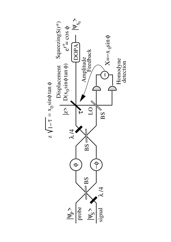
FIG. 1.: Setup for QND measurements of a field quadrature on the state $|\psi_{\sc s}\rangle$. The signal is linearly mixed with a probe mode in a Mach-Zehnder interferometer, which, equipped with two additional $\lambda/4$ plates, shows a transmittivity $\cos^{2}\phi$. Such transmittivity can be tuned by varying the internal phase-shift $\phi$. One of mode exiting the interferometer is then revealed by homodyne detection, and the resulting outcome $x_{0}$ is used for a feedback-assisted displacement, by an amount $x_{0}\sin\phi\tan\phi$ of the other mode. Such displacement is obtained by mixing the mode with a strong coherent state of amplitude $z$ (e.g. the laser beam also used as local oscillator for the homodyne detector) in beam splitter of transmittivity $\tau$ close to unit, with the requirement that $z\sqrt{1-\tau}=x_{0}\sin\phi\tan\phi$. Finally, the conditional output is squeezed by a degenerate parametric amplifier (DOPA) by an amount $S(r^{\star})$ with $e^{r^{\star}}=\cos\phi$. By varying the degree of squeezing of the probe mode the resulting measurement ranges from a projective to a fully non-destructive detection of the field quadrature.

REFERENCES

- [1] J. von Neumann, Mathematical Foundations of Quantum Mechanics (Princeton Univ. Press, Princeton, NJ, 1955), pp. 442-445.
- [2] M. D. Levenson et al, Phys. Rev. Lett. 57, 2743 (1986).
- [3] A La Porta et al, Phys. Rev. Lett. 62, 28 (1989).
- [4] S. Pereira et al, Phys. Rev. Lett. 72, 214 (1994).
- [5] J. Poizat, P. Grangier, Phys. Rev. Lett. 70, 271 (1993).
- [6] S. R. Friberg, Phys. Rev. Lett. 69, 3165 (1992).
- [7] R.Bruckmeier et al, Appl. Phys. B 64, 203 (1997).
- [8] F. X. Kartner, H. A. Haus, Phys. Rev. A 47, 4585 (1993); Appl. Phys. B 64, 219 (1997).
- [9] K. Jacobs et al, Phys. Rev. A 49, 1961 (1994).
- [10] M. Pinard et al, Phys. Rev. A 51, 2443 (1995).
- [11] G. M. D’Ariano, M. F. Sacchi, Phys. Lett. A 231, 325 (1997).
- [12] M. G. A. Paris, Phys. Lett. A 217, 78 (1996).
- [13] P. K. Lam et al, Phys. Rev. Lett. 79, 1471 (1997).
- [14] K. Banaszek, Phys. Rev. Lett. 86, 1366 (2001)
- [15] M. G. A. Paris, unpublished.
- [16] D. Walls and G. Milburn, Quantum optics Springer Verlag (Berlin, 1994).
- [17] C. Fuchs, A. Peres, Phys. Rev. A 53, 2038 (1996).
- [18] M. Ozawa, Publ. RIMS Kyoto 21, 279 (1985).
- [19] H. F. Hofmann, Phys. Rev. A 61, 033815 (2000).