Fast, efficient error reconciliation for quantum cryptography

Abstract

We describe a new error reconciliation protocol Winnow based on the exchange of parity and Hamming’s “syndrome” for $N-$bit subunits of a large data set. Winnow was developed in the context of quantum key distribution and offers significant advantages and net higher efficiency compared to other widely used protocols within the quantum cryptography community. A detailed mathematical analysis of Winnow is presented in the context of practical implementations of quantum key distribution; in particular, the information overhead required for secure implementation is one of the most important criteria in the evaluation of a particular error reconciliation protocol. The increase in efficiency for Winnow is due largely to the reduction in authenticated public communication required for its implementation.

I Introduction

Quantum cryptography [1] presents special problems in regard to error correction of noisy quantum communications. Under the constraint that the public channel can be authenticated, and the assumption that all public communications can be eavesdropped, classical information on the exchanged qubits must be revealed through a series of public discussions to test the quantum key integrity and to remove the errors. Discrepancies within the qubits, observed as errors, must be treated as having been introduced by a hostile eavesdropper; the eavesdropper is generally referred to as Eve and labeled E in this work.

In a classical environment all errors can always be removed with the condition that to remove all errors one may have to reveal all information. However, within the secrecy framework imposed by quantum key distribution (QKD), revealed information reduces privacy and the effective channel capacity. Because of this great care must be taken to reveal a minimal amount of information to remove errors from quantum key while accounting for the leaked information to ensure key integrity after errors are removed.

Within this context of QKD, the two parties that exchange qubits over a quantum channel (Alice (A) and Bob (B) is the notation typically used within the quantum cryptography community) must have a fast and efficient method to mend the quantum key; in addition, they must also reduce E’s knowledge gained during public discussions to a vanishingly small amount. These constraints require that any error reconciliation protocol will also need supporting protocols to provide a complete framework for quantum cryptographic security. That is, a useable QKD system will comprise a quantum-key transmitter (A) and receiver (B), and a series of protocols to remove errors and account for and mitigate the information leakage attributable to E. The series of protocols includes [2, 3], but is not necessarily limited to the following: error-reconciliation [4, 5], privacy amplification [6] and signature authentication [7].

In addition to these protocols, we acknowledge a protocol generally formulated in [4] that we refer to as privacy maintenance. We also note that the predecessor to CASCADE [5] — the best known and probably the most widely used error reconciliation protocol — is also generally formulated in [4] and is characterized by a binary search; here we refer to the binary search, which is a major element of CASCADE, as BINARY. A fundamental difference between BINARY and CASCADE is that CASCADE neglects privacy maintenance: all data are retained until the necessary privacy amplification is performed on the error-free data. We observe that the reconciliation process is more efficient if privacy maintenance is implemented during reconciliation as will become obvious in the following discussion.

Finally, this work introduces a new error reconciliation protocol that uses a Hamming code [8, 9] to remove errors. We refer to this protocol as Winnow. Winnow is characterized by the application of a parity test, a conditional Hamming hash, and privacy maintenance.

II Hamming Error Detection and Correction

The application of the Hamming hash function for error correction [8, 9] is illustrated as follows:

First, after A and B exchange qubits on the quantum channel, A and B then divide their random bits into blocks of length $N_{h}=2^{m}-1$. (Due to the 1:1 correlation of these data, we henceforth refer to these blocks as a single data- or bit-block.) The $m-$bit ($m\geq 3$) syndromes $S_{a}$ and $S_{b}$ are then calculated, where $S_{a}$ and $S_{b}$ respectively depend only on A’s or B’s bits in a particular block.

Next, B transmits his syndrome to A and errors are only discovered if the syndrome difference $S_{d}$ (exclusive or of $S_{a}$ with $S_{b}$) is non-zero:

$$S_{d}=S_{a}\oplus S_{b}\neq\{0\}^{m}\text{.}$$ (1)

Finally, $m$ bits are deleted from each bit block to eliminate the potential loss of privacy to E due to the (classical) communication of B’s syndromes: $m$ bits of information are revealed on each block for which $S_{b}$ is revealed reducing the channel capacity per symbol by $m/N_{h}$[10].

Specifically, data privacy is maintained by removal of $m$ bits from each block at the $\{2^{j}\}$ positions where $j\in\{0,\ldots,m-1\}$. These bits are independent in the syndrome calculations as seen below in the matrix $h^{(m)}$:

$$h^{(3)}=\left[\begin{array}[]{ccccccc}1&0&1&0&1&0&1\\ 0&1&1&0&0&1&1\\ 0&0&0&1&1&1&1\\ \end{array}\right]\text{,}$$ (2)

where for this particular matrix, $m\equiv 3$. We refer to the operation of discarding bits in this manner [4] as privacy maintenance.

As a final comment on Eq. 2, note that the transpose of $h^{(3)}\equiv\left[h^{(3)}\right]^{T}$ are the binary equivalent numbers $1$ to $7$, and is generalized such that $[h^{(m)})]^{T}\equiv\{1,\ldots,(2^{m}-1)\}$, $N_{h}$ binary numbers.

The matrix $h^{(m)}$ is a special form of hash function [11] and is represented by:

$$h^{(m)}_{i,j}=\left\lfloor{j\over 2^{i-1}}\right\rfloor\left({\rm mod}\;2\right)\text{,}$$ (3)

where $i\in\{1,\ldots,m\}$, and $j\in\{1,\ldots,N_{h}\}$; arithmetic is modulo 2.

The Hamming algorithm always corrects any single error within any $N_{h}$-bit block, but the effect of the Hamming algorithm, which is related to the syndromes and privacy maintenance, is less clear in the event that more than one error exists in a bit block. Such considerations are now discussed in detail in terms of the syndromes.

The syndromes $S_{a}$ and $S_{b}$ are formed by contraction of the $N_{h}-$bit blocks with the matrix $h^{(m)}$:

$$S_{i}=\left(\sum_{j=1}^{N_{h}}X_{j}h^{(m)}_{i,j}\,\right)\left({\rm mod}\;2\right)\in\{0,1\}^{m}\text{,}$$ (4)

where subscript $i$ represents syndrome bit $i$ in the $m$-bit binary syndrome, $X_{j}$ represents bit j $\in$ A’s or B’s block, and $S=\{S_{i}\}$ is the binary syndrome value of either B’s or A’s block. Understanding the effect of the syndromes in locating and correcting errors is crucial to assessing the performance of Hamming, and thus Winnow.

The syndrome difference (Eq. 1) defines a binary number that gives the location of a single bit in A’s or B’s code word that when toggled from $0\mapsto 1$ or from $1\mapsto 0$ affects the syndrome difference $S_{d}$ such that when the syndrome difference is recalculated it gives the binary number $S_{d}^{\prime}\equiv\{0\}^{m}$. For example, if $S_{d}\neq\{0\}^{m}$, then $S_{d}$ is an $m$-bit binary number whose value gives the location of a single bit in either A’s or B’s code-word to add exclusive or with the orignal bit value. After that bit value is changed, then the new syndrome for that code word is then calculated (e.g. $S_{A}^{\prime}$) and added (again, exclusive or) to the original syndrome for the other code word ($S_{B}$ in this example). The result is that the changing of the single bit indicated by the non-zero syndrome difference in the one code-word either corrects an error, or introduces another, in that code word. This is no great mystery but rather reflects the fact that Hamming codes are n-k codes. In this case, $n=2^{m}-1$ relates the number of bits in each code word ($N_{h}$), and $k=n-m$ relates the channel capacity (the channel capacity is $k/n\Longleftrightarrow k/N_{h}$ per bit) given the code (a Hamming code in this discussion).

In an n-k Hamming code, there are $2^{(2^{m})}$ unique code words characterized by $2^{m}$ unique syndromes; further, there are $2^{k}$ code words with the same syndrome. Because this code can correct $1$ error, it has a minimum Hamming distance of $d=3$. This also means it can detect at least $2$ errors. In fact the Hamming distance $d$ for the Hamming code is $d\equiv 3$.

By definition, a code word with a single error will have $S_{d}\neq\{0\}^{m}$ (can obviously detect a single error if it can correct a single error). In addition, if a code word has exactly $2$ errors then by definition $S_{d}\neq\{0\}^{m}$ (can detect at least $2$ errors if it can correct a single error). Therefore, if a code word has exactly $2$ errors, then after applying the Hamming algorithm, and after changing the bit value indicated by $S_{d}$, the code word will finish with exactly $3$ errors. The proof is by contradiction: If a code word with $2$ errors finished with $1$ error (an error was corrected), then the new syndrome difference would be non-zero! Contradiction also proves that $1$-error is corrected if there is exactly $1$ error: If an error was introduced the syndrome difference would again be non-zero. Thus, in examining Hamming codes we observe that a code word with $1$ error will finish with $0$ errors, but a code word with exactly $2$ errors finishes with exactly $3$ errors. In each case the new syndrome difference changes such that $S_{d}^{\prime}=\{0\}^{m}$.

By symmetry, if an $N_{h}$-bit code word contains exactly $N_{h}-1$-errors (all the bits except one are in error), then after application of Hamming all the bits in the code word will be in error. Further, a code word that contains $N_{h}-2$ errors will finish with $N_{h}-3$ errors, i.e one of the errors is corrected.

The above arguments imply that a Hamming code only works well if the probability of $2$ or more errors is low relative to the liklihood of a single, or no, errors. In either case the Hamming code is inefficient as $m$-bits are revealed in the syndrome (this fact is discussed in detail later).

The difficult question to answer in analyzing the performance of a Hamming code is how does Hamming affect code words with more than $2$, but less than $2^{m-1}$, errors?

It is not obvious but the number of code words with $3$-errors and $S_{d}\equiv\{0\}^{m}$ is related to the number of ways $2$-error code words map to a code word with $3$ errors (and $S_{d}=\{0\}^{m}$). In other words, there must be a way to arrange $3$ errors in a code word and still maintain $S_{d}=\{0\}^{m}$. Lacking this would mean that the code could always detect more than $2$ errors with a Hamming distance of $d=3$.

To complete the Hamming efficiency analysis, how code words with $3$ or more errors are affected after application of Hamming must be analyzed. For $3$ errors it is now obvious: there must be at least $2^{m}-1$ ways to start with $3$ errors in an $N_{h}$-bit code word and still finish with $3$ errors. In the case that there exist $3$ errors in a code word, and $S_{d}\neq\{0\}^{m}$, then an error will be introduced into the $N_{h}$-bit code word because if the code word finished with $2$ errors then $S_{d}\neq\{0\}^{m}$—a contradiction.

As a special case (example), consider $m=3$. There are ${7\choose 3}=35$ ways to arrange $3$ errors in $7$ bits. Because there are exactly $7$ non-zero syndrome differences for $m=3$ and $n_{i}=2$, there must be at least $7$ ways to arrange $3$ errors in $7$-bits and have $S_{d}\equiv\{0\}^{m}$. In fact for this special case this is the result. What this means is that, statistically, $7$ in $35$ code words with $3$-errors will finish with $3$-errors, and $28$ in $35$ words with $3$ errors will finish with $4$ errors. Thus, code words that start with $3$ errors will finish with $19/5$ errors per $7$-bit block, in the limit of an infinite number of $7$-bit blocks with exactly $3$ errors. By symmetry, it is obvious that given an infinite number of $7$-bit blocks with exactly $4$ errors, the final error rate per block would be $16/5$—a lower final error rate.

Thus, what is needed is a way to calculate, for any number $m$ of parity checks, in Hamming, a way to calculate the number of ways to arrange the initial number of errors per block and finish with $S_{d}=\{0\}^{m}$, or with $S_{d}\neq\{0\}^{m}$. Eq. 7 permits that calculation for any initial number of errors per block, $n_{i}$, given any initial block size, $N_{h}$:

$$N_{S_{d}\neq 0}+N_{S_{d}=0} = {N_{h}\choose n_{i}}$$ (5)

$$-N_{S_{d}\neq 0}+N_{h}\cdot N_{S_{d}=0} = (-1)^{q}\cdot N_{h}\cdot{\frac{N_{h}-1}{2}\choose p}$$ (6)

$$\Longleftrightarrow{\left[\matrix{N_{S_{d}\neq 0}\cr N_{S_{d}=0}}\right]} = \left[\matrix{N_{h}&1\cr-1&1\cr}\right]^{-1}\left[\matrix{{N_{h}\choose n_{i}}\cr(-1)^{q}{\frac{N_{h}-1}{2}\choose p}\cr}\right]\text{,}$$ (7)

where $q=\lceil n_{i}/2\rceil$, $p=\lfloor n_{i}/2\rfloor$, $n_{i}$ is the initial number of errors per Hamming block of $N_{h}=2^{m}-1$ bits per block; in this situation, $N_{S_{d}=0}$ gives the number of syndrome differences with $S_{d}=\{0\}^{m}$, and $N_{S_{d}\neq 0}$ gives the number of syndrome differences with $S_{d}\neq\{0\}^{m}$. Eq. 7 is generalized by dividing both sides by the total number of ways to arrange $n_{i}$ errors in the $N_{h}$ bits. In this situation we find a more useful quantity:

$$\Pi_{S_{d}=0} = \frac{N_{S_{d}=0}}{{N_{h}\choose n_{i}}}\text{, and}$$ (8)

$$\Pi_{S_{d}\neq 0} = \frac{N_{S_{d}\neq 0}}{{N_{h}\choose n_{i}}}\text{.}$$ (9)

This result is required later.

These arguments are not obviously general for the case of $m>3$, but they give insight into the general problem. The difficulty with the special case of $m=3$ and $n_{i}=3$ is that the next case of $n_{i}=4$ is symmetric and complementary with $n_{i}=3$, as mentioned previously. Further, as was noted, there is no path to map $3$ errors to $2$ errors as $S_{d}\neq\{0\}^{m}$ when there are exactly $2$ errors. However, Eq. 7 is the general technique to calculate the quantities specified, i.e. the number of ways to map $n_{i}$ errors to $S_{d}=\{0\}^{m}$ or not, given $N_{h}=2^{m}-1$ bits in a block.

Given these facts, how the errors change for $m\geq 4$ and $4\leq n_{i}<2^{(m-1)}$ is the general result of interest.

Let $n_{i}^{(+)}$ be the number of ways to increase the number of errors from $n_{i}$ to $n_{i}+1$, in a bit-block, and $n_{i}^{(-)}$ the number of ways to decrease the number of errors from $n_{i}$ to $n_{i}-1$; of course, the considerations relate to $m\geq 4$. The results are as follows:

$$n_{i}^{(+)} = N_{S_{d}=0}(N_{h}|n_{i})+(n_{i}+1)\cdot N_{S_{d}=0}(N_{h}|n_{i}+1)$$ (10)

$$n_{i}^{(-)} = {N_{h}\choose n_{i}}-n_{i}^{(+)}\text{,}$$ (11)

where $N_{S_{d}=0}(N_{h}|n_{i}+1)$ is the number of ways to arrange $n_{i}+1$ errors in $N_{h}$ bits and obtain $S_{d}=\{0\}^{m}$ (the reader will recall that earlier it was stated that the number of ways to get $S_{d}=\{0\}^{m}$ for $n_{i}+1$ errors is directly related to the number of ways to map $n_{i}\mapsto n_{i}+1$ errors); of course, $N_{S_{d}=0}(N_{h}|n_{i})$ is the number of ways to arrange $n_{i}$ errors in $N_{h}$ bits and get $S_{d}=\{0\}^{m}$. Thus, the generalized probability for the number of errors $n_{i}$ to increase, or decrease is:

$$\Pi^{(+)} = \frac{n_{i}^{(+)}}{n_{i}^{(+)}+n_{i}^{(-)}}\text{, and}$$ (12)

$$\Pi^{(-)} = 1-\Pi^{(+)}\text{.}$$ (13)

III Winnow

As a general rule, the ideal error correcting protocol would correct all bit errors in each bit block, introduce no additional bit errors, and reveal a minimal amount of information on the key bits to an eavesdropper through public communication. The outlined Hamming protocol has a number of shortcomings regarding this ideal. First, the difference syndrome $S_{d}$ does not distinguish between single- and multiple-bit errors. Therefore, additional errors may be introduced if instances of $S_{d}\neq\{0\}^{m}$ are treated as due to single errors. Second, up to $m$ bits of information are exchanged for each data block reducing channel capacity per symbol with each exchange: information which can be compromised by eavesdropping.

One solution is to eliminate all bits within data blocks for which $S_{d}\neq\{0\}^{m}$. This certainly removes the possibility of introducing additional bit errors into the key, but, unfortunately, the efficiency of such a method is low as every block loses either $m$-bits to privacy maintenance, or all bits because $S_{d}\neq\{0\}^{m}$. The efficiency of this approach is not optimal as most of the discarded bits/blocks for which $S_{d}\neq\{0\}^{m}$ are probably not in error.

Another, more powerful solution is to introduce a preliminary parity comparison on a block of $N=2^{m}$ bits and to make a comparison of the syndromes $S_{a}$ and $S_{b}$ conditional upon the result of the parity comparison.

If the block parities do not agree an odd number of errors exists in the $N$-bit block. Moreover, if the bit errors are distributed randomly throughout the data, and if the number of errors is sufficiently small, then an odd number of errors in a block probably indicates a single error which can be corrected by the additional application of the Hamming algorithm. For example, in the situation that a block contains one bit error, if $S_{d}=\{0\}^{m}$ then the first bit is in error. (By symmetry it is clear that if there are exactly $N-1$ errors in the block the first bit would not be in error.) Thus, this approach always allows the correction of a single error in the $N$ bits, i.e. if the bits are to be retained. However, in the protocol outlined here the one bit is regularly discarded for privacy maintenance (for the exchanged parity bit) and the Hamming algorithm is applied to the remaining $N_{h}$ bits, as previously discussed, and then $\lceil\log_{2}(N_{h})\rceil$ additional bits are discarded to complete the privacy maintenance giving a channel capacity of $(2^{m}-m-1)/N$ per symbol on blocks that contain an initial parity error. This appears to be an additional loss of channel capacity, but because the syndromes are not exchanged and compared when the block parities agree the channel capacity actually increases over the basic Hamming algorithm; one bit is still discarded from the blocks that do not exhibit a parity error for privacy maintenance. We refer to this error reconciliation protocol as Winnow.

Winnow reveals $\log_{2}(N)+1$ bits in $2$ classical communications when the parities on the $N$ bits do not agree: $m$ bits for the syndrome and $1$ bit for parity; conversely, Winnow reveals $1$ bit of information in $1$ classical communication when the parities agree.

Therefore, the amount of key data discarded is

$$N^{odd}_{dis.}=\log_{2}(N)+1=m+1$$ (14)

bits for blocks with odd numbers of errors such that the fraction of the bits remaining after privacy maintenance is

$$\mu^{odd}_{pm}=1-\frac{N^{odd}_{dis.}}{N}\text{.}$$ (15)

For $N\in\{8,16,32,64,128\}$, $\mu^{odd}_{pm}\in\{0.5,0.69,0.88,0.89,0.94\}$, respectively. Also,

$$\mu^{even}_{pm}=1-\frac{1}{N}\text{,}$$ (16)

and $\mu^{even}_{pm}\in\{0.88,0.94,0.97,0.98,0.99\}$ for the same values of $N$. In either case, the appropriate overhead for the classical communications is also removed immediately from the data so that the privacy of the bits is at least maintained if not improved.

All single bit errors in an $N$-block are guaranteed to be either eliminated or corrected after a single pass of Winnow (a Winnowing). What remains to be considered is how blocks with multiple errors affect the overall efficiency of Winnow.

IV Winnow Efficiency

Define the change in number of errors in a given block and for a given initial number of errors as $\Delta n=n_{f}-n_{i}$, where $n_{i}$ and $n_{f}\equiv n_{f}(n_{i}|N)$ are the initial and final numbers of bit errors in a block prior to and after Winnowing, respectively. The average change in the number of errors, for a given number of initial errors, after a Winnowing (this step includes elimination of the parity bit but not the final $m$-bits required for completion of the privacy maintenance step) can be expressed as

$$\bar{\Delta n}\equiv\big{\langle}\!\Delta n(n_{i})\!\big{\rangle}=\sum_{\Delta n=-2}^{1}\Delta n\!\cdot\!p(\Delta n|n_{i})\text{,}$$ (17)

where

$$\sum_{\Delta n=-2}^{1}p(\Delta n|n_{i})=1\text{,}$$ (18)

and $p(\Delta n|n_{i})$ is the probability that the number of errors will change by $\Delta n\in\{-2,-1,0,1\}$ given an initial condition of $n_{i}$ errors in an $N-$bit data block. The $p(\Delta n|n_{i})$ of interest can be written more instructively as

$$p(\!+1|n_{i})\! = \!\pi^{(n)}\!\!\cdot\!\Pi_{S_{d}\neq 0}(n_{i})\!\cdot\!\Pi^{(\!+\!)}(n_{i})$$ (19)

$$p(\!\pm 0|n_{i})\! = \!\pi^{(n)}\!\!\cdot\!\Pi_{S_{d}=0}(n_{i})\!+\!\pi^{(y)}\!\cdot\!\Pi_{S_{d}\neq 0}(\delta n_{i})\!\cdot\!\Pi^{(\!+\!)}(\delta n_{i})$$ (20)

$$p(\!-1|n_{i})\! = \!\pi^{(n)}\!\!\cdot\!\Pi_{S_{d}\neq 0}(n_{i})\!\cdot\!\Pi^{(\!-\!)}(n_{i})+\pi^{(y)}\!\cdot\!\Pi_{S_{d}=0}(\delta n_{i})$$ (21)

$$p(\!-2|n_{i})\! = \!\pi^{(y)}\!\!\cdot\!\Pi_{S_{d}\neq 0}(\delta n_{i})\!\cdot\!\Pi^{(\!-\!)}(\delta n_{i})\text{,}$$ (22)

where, $n_{i}$ is as previously defined, $\delta n_{i}\equiv n_{i}-1$, $\pi^{(y\vee n)}$ depends only on the initial number of errors ($n_{i}$) in the $N$-bit block and is the probability the bit discarded for privacy maintenance following the parity check was (y), or (^∨) was not (n) in error; $\Pi_{S_{d}=0}(n_{i}^{\vee}\delta n_{i})$ and $\Pi_{S_{d}\neq 0}(n_{i}^{\vee}\delta n_{i})$ are the probabilities that $S_{a}\!=\!S_{b}$ or $S_{a}\!\neq\!S_{b}$ for $n_{i}$ or $\delta n_{i}$ errors in $N_{h}$ bits and are concretely defined in Eq. 9, and $\Pi^{(\pm)}(n_{i}^{\vee}\delta n_{i})$ is defined in Eq. 13.

Eq. 17 can be expressed in terms of $\pi^{(y\vee n)}$, $\Pi_{S_{d}}$ and $\Pi^{(\pm)}$ as

$$\bar{\Delta n} \equiv \big{\langle}\!\Delta n^{(n)}(n_{i})\!\big{\rangle}+\big{\langle}\!\Delta n^{(y)}(n_{i})\!\big{\rangle}\text{,}$$ (23)

$$= \bar{\Delta n}^{(n)}+\bar{\Delta n}^{(y)}\text{,}$$ (24)

where the arguments which depend on $n_{i}$ have been suppressed, and

$$\bar{\Delta n}^{(n)}\!\! = \pi^{(n)}\!\!\cdot\!\Pi_{S_{d}\neq 0}(n_{i})\!\cdot\!\Big{[}1\!-\!2\!\cdot\!\Pi^{(-)}(n_{i})\Big{]}\text{,}$$ (25)

$$\bar{\Delta n}^{(y)}\!\! = \pi^{(y)}\!\cdot\!\Pi_{S_{d}\neq 0}(\delta n_{i})\!\cdot\!\Big{[}1\!-\!2\!\cdot\!\Pi^{(-)}(\delta n_{i})\Big{]}\!-\pi^{(y)}\text{.}$$ (26)

The final quantity needed to calculate the efficiency of Winnow is $\pi^{(y\vee n)}$:

$$\pi^{(y)} = \frac{n_{i}}{N}\text{, where}$$ (27)

$$\pi^{(y)}+\pi^{(n)} = 1\text{.}$$ (28)

Table I and Table II provide a concrete example for the special case of $m=3$ of the effects of Winnow on blocks with exactly $n_{i}\in\{0,\ldots,8\}$ errors. Table I, introduces a new quantity

$$\bar{n}_{f}\equiv\langle n_{f}\rangle=n_{i}+\bar{\Delta n}\text{,}$$ (29)

and in Table II a new parameter

$$p_{f}=\frac{\bar{n}_{f}}{N_{f}}$$ (30)

is defined.

The parameter $p_{f}$ defines the probability for each bit in a given block to be in error. The number $N_{f}\in\{N-1,N-m-1\}$ and its value depends on the action required by Winnow for a given number of initial errors. For example, $N_{f}=N-1$ or $N-m-1$ for $p_{f}$ and $n_{i}$ even or odd, respectively.

These two tables illustrate the effect of Winnow on data which are divided into 8-bit blocks. The values marked with superscript $p$ reflect the effect of discarding one bit following the parity comparison. The values marked with superscript $ph$ refer to the data after the Hamming algorithm is also applied, but before the requisite $\log_{2}(N)=3$ bits of data are discarded for privacy maintenance. The final values denoted by subscript $f$ reveal the effect of Winnow (including the effect of all discarded data required for privacy maintenance).

The parameter $p_{f}$ clearly shows a reduction in errors for $n_{i}=1$ and an increase in errors for $n_{i}=3$. It also shows that discarding data to maintain privacy of the remaining key has no effect on the error probability.

The fraction of key remaining after a Winnowing is given by

$$\mu_{N}\equiv\frac{\langle N_{f}\rangle}{N}=\frac{\sum_{n_{i}=0}^{N}\,N_{f}\,P(n_{i}|N)}{N}\text{,}$$ (31)

and the probability for any key bit to be in error following a Winnowing is

$$p_{N}=\frac{\langle\bar{n}_{f}\rangle}{\langle N_{f}\rangle}=\frac{\sum_{n_{i}=0}^{N}\bar{n}_{f}(n_{i})\!\cdot\!P(n_{i}|N)}{N\!\cdot\!\mu_{N}}\text{,}$$ (32)

where $P(n_{i}|N)$ is the probability for an $N$-bit block to contain $n_{i}$ errors before a Winnowing.

Obviously, the efficiency with which Winnow removes errors depends upon the distribution of errors within the data. Without intimate knowledge of a specific QKD apparatus, a reasonable assumption is that the errors are random and normally distributed throughout the data. Given this assumption, $P(n_{i}|N)$ in Eq. 32 is given by the binomial distribution

$$P(n_{i}\mid N,p_{0})={N\choose n_{i}}{p_{0}}^{n_{i}}(1-p_{0})^{N-n_{i}}$$ (33)

where $p_{0}$ is the probability that any given bit is in (relative) error.

With this assumption, Eqs. 31 and 32 can be expressed as

$$\mu_{N}=\frac{N-1-m\sum_{n_{i}^{odd}}{N\choose n_{i}}{p_{0}}^{n_{i}}(1-p_{0})^{N-n_{i}}}{N}\text{,}$$ (34)

where $m=\log_{2}(N)$, and

$$p_{N}=\frac{\sum_{n_{i}=0}^{N}\bar{n}_{f}(n_{i}){N\choose n_{i}}{p_{0}}^{n_{i}}(1-p_{0})^{N-n_{i}}}{N\!\cdot\!\mu_{N}}\text{.}$$ (35)

The efficiency with which Winnow reduces errors in the key is of great interest. Two related issues which concern the efficiency are: 1) the number of iterations of Winnow necessary to achieve a sufficiently low probability of error in the remaining key data, and 2) the amount of key data that is discarded through privacy maintenance.

The number of iterations is of concern because each iteration reveals information and consumes time with each communication between A and B. Moreover, each communication requires the use of some private key for signature authentication [7]. Most importantly, though, is that each iteration requires a significant amount of data to be discarded through privacy maintenance.

Smaller $N$ require more data to be discarded than larger $N$ as can be seen from Eq. 34. However, an effect which tends to mollify this undesirable condition is that smaller $N$ are more efficient at removing errors for larger values of initial error probability. This effect is illustrated in Fig. 1 where we have plotted $p_{N}/p_{0}$ for several values of $N$. For all values of $N$ and $p_{0}$ sufficiently small, $p_{N}/p_{0}<1$ and the protocol can remove errors from the key data. However, as $p_{0}$ increases from $p_{0}=0$, each of the curves passes through $p_{N}/p_{0}=1$ indicating that additional errors are being introduced into the key. Moreover, the value of $p_{0}$ for which $p_{N}/p_{0}=1$ is smaller for larger N and the curves do not intersect between $p_{0}=0$ and $p_{N}/p_{0}=1$.

As a primary requirement of Winnowing real data in an iterative application, a random shuffling of the data between iterations is essential to randomly redistribute missed or introduced errors. Without this random shuffle multiple errors remain clumped together and, in essence, are impossible to completely remove from the data. Under this constraint it is obvious that the final error probability, and the amount of data remaining after a number of Winnowings, depends on the way in which $N$ is varied throughout the successive Winnowings. An intuitive result which we have verified empirically is that less data are discarded for the same initial and final error probabilities if $N$ is chosen well for the first iteration and is either held constant or increased for all subsequent iterations; there is no advantage to decreasing $N$ in subsequent iterations if Winnow is applied as outlined here.

Define

$$p(p_{0};\{j_{N}\})$$ (36)

and

$$\mu(p_{0};\{j_{N}\})$$ (37)

as the final error rate and fraction of data remaining after a sequence $\{j_{N}\}=\{j_{8},j_{16},j_{32},j_{64},j_{128}\}$ where $j_{N}$ iterations of Winnow are applied with a block size $N\in\{8,16,32,64,128\}$ beginning with $N=8$ and increasing monotonically in $N$ by factors of $2$.

Because $(p_{8}<p_{0})\;{\forall}\;(p_{0}<0.5)$, it may appear that errors can be corrected in the data for this entire range of initial error probability. However, there is another criterion that must be met which significantly reduces the maximum correctable error probability: There must remain a finite amount of error-free data after the potential information possessed by E is reduced through privacy amplification.

The maximum amount of potential information possessed by E can be determined by the initial error probability $p_{0}$ and depends on the QKD protocol and the type of attacks being employed. For example, if the BB84 protocol is used and E employs a complete intercept/resend attack on the quantum channel in the same bases used by B, she will introduce an error probability of $p_{0}=1/4$. She will also potentially know $1/2$ of the data before error reconciliation and up to $2/3$ of the data which remains after error reconciliation.

If E uses a more clever intercept/resend strategy of detecting and resending in the Breidbart basis (second paper in [4]), she would introduce the same number of errors ($p_{0}=1/4$) and could know up to a fraction of $0.59$ of the data before error reconciliation and $0.78$ of the data remaining after error reconciliation.

It should also be noted that certain states of light are more susceptible to attack than others. For example, consider weak coherent states which are commonly used in QKD systems. If E also employs a beamsplitter attack [3, 4, 12] against one of these systems, an additional amount of data is compromised which is not greater than the mean number of photons in the state. However, this value can be made arbitrarily small so it is neglected in the following calculations. Moreover, other states of light can be used in QKD schemes which are not vulnerable to this type of attack [13].

Thus, the fraction of data remaining after error reconciliation and privacy amplifications can be

$$\nu^{bb84}=\mu-(0.59)4\,p_{0}$$ (38)

for BB84, where $\nu$ describes the remaining fraction of key.

From the above considerations, $p$ and $\nu$ can be investigated as a function of $p_{0}$. Of particular interest is the maximum $p_{0}$ for which some secure data remains while achieving a sufficiently low final error probability to make the data useful. We have chosen, somewhat arbitrarily, $p\leq 10^{-6}$ as a reasonable target for the final error probability.

With this target and the remaining fraction of private data described by Eq. 38, we find the largest initial error probability for which some private data remains is

$$p_{0}=0.1322\text{,}$$ (39)

after Winnowing and privacy amplification.

To achieve $p\lesssim 10^{-6}$ from this large initial error probability, Winnow must be applied in the sequence $\{j_{N}\}=\{3,1,0,1,3\}$. That is, $3$ Winnowings with $N=8$ must be followed by $1$ Winnowing with $N=16$, etc. If this prescription is followed,

$$\nu^{bb84}=0.0017$$ (40)

of the original data remain and are secure following privacy amplification.

Some QKD schemes require a larger estimate of E’s knowledge. If Eq. 38 is replaced with [4]

$$\nu=\mu-2\sqrt{2}\,p_{0}\text{,}$$ (41)

we find

$$p_{0}=0.1222$$ (42)

for $\{j_{N}\}=\{3,0,1,0,4\}$. This leaves a fraction $\nu=0.0017$ of the original data as secure data with a single-bit error probability $\leq 10^{-6}$.

Finally, if we estimate that E knows every bit of data by causing $p_{0}=1/4$, then

$$\nu=\mu-4\,p_{0}\text{.}$$ (43)

We then find that the largest reconcilable $p_{0}$ is

$$p_{0}=0.1037$$ (44)

for $\{j_{N}\}=\{2,1,1,0,3\}$ and $\nu=0.0020$.

The most efficient iteration sequence ($\{j_{N}\}$) for any QKD scheme can be determined by first applying Winnow with $N=8$ to estimate $p_{0}$. Once the number of blocks with odd and even (even includes zero) errors, $M^{odd}_{e}$ and $M^{even}_{e}$ respectively, are known, the fraction

$$\frac{\#\text{ of Parity Errors}}{\#\text{ of Blocks}}=\frac{{\sum_{n_{i}^{odd}}{N\choose n_{i}}{p_{0}}^{n_{i}}(1-p_{0})^{N-n_{i}}}}{N}$$ (45)

can be used to estimate $p_{0}$. Knowledge of $p_{0}$ is sufficient to determine the $\{j_{N}\}$ which maximizes $\nu$.

For small $p_{0}$, the most efficient $\{j_{N}\}$ may start with $N>8$. However, working systems that have been reported in the literature [4, 14] have large enough error probabilities so that the most key is left if $N=8$ for at least the first iteration.

A detailed analysis of the advantages of Winnow over other protocols is beyond the scope of this work. However, it is instructive to note the advantages over at least the best-known protocol CASCADE.

The most notable difference between Winnow or BINARY and CASCADE is that CASCADE does not employ privacy maintenance. The disadvantage of such a protocol is that super-redundant information must be exchanged with each successive iteration. This is to be compared with BINARY and Winnow which reduce the size of the data set with each communication. With the reasonable requirement that a bit revealed through these communications requires at least a bit to be eliminated through some channel, either before or during privacy amplification, then the inefficiency of keeping all bits until all errors are removed becomes obvious: retaining and repetitively exchanging information on the same bits is an additional expense to the protocol.

For the purpose of comparison, we have computed the maximum $p_{0}$ which BINARY (less privacy maintenance) can successfully reconcile errors and preserve a small amount of secure data after privacy amplification and the removal of the super-redundant information. We find

$$p_{0}=0.114$$ (46)

for $\{j_{N}\}=\{2,1,0,2,1\}$ and $\nu^{bb84}=0.01$ when $(0.59)4\,p_{0}$ describes the additional amount of key that must be discarded through privacy amplification. This is to be compared with $p_{0}=0.1322$ for the same considerations with Winnow. This application of BINARY is a reasonable approximation to CASCADE which may include a higher order correction giving a slightly higher overall error reduction than BINARY without privacy maintenance.

This comparison (or any of the previous discussion) does not take into account bits used to authenticate messages sent between A and B. Both CASCADE and BINARY requires significantly more two-way communication than Winnow, and each packet of $n$ bits sent may require $\lceil\log_{2}(n)\rceil$ for authentication [7]. We calculate that the most efficient application of CASCADE requires a minimum of $1+\log_{2}(N)$ communications per iteration while Winnow requires only $2$ communications for any block size $N$ that exhibits a parity error; the additional communications required imposes a tight limitation on practical efficiency. In addition, because CASCADE does not maintain privacy, subsequent iterations requires more bits to be exchanged in the initial parity phase with each iteration. The additional bit exchanges may require additional signature authentication bits.

We acknowledge that because CASCADE and BINARY always removes a single error and never introduces additional errors to multiple error blocks, both BINARY and CASCADE perform infinitesimally better than Winnow in an environment where signature authentication is not required and privacy maintenance is removed from the Winnow and BINARY protocols. However, Winnow’s $2$ communications is a great advantage where time is of the essence with regard to production of secure key bits over inefficient noisy quantum channels.

V Conclusion

We have identified a new, fast, efficient, error reconciliation protocol for quantum key distribution which requires only $2$ communications between the two parties attempting to reconcile private, quantum key material. We refer to this protocol as Winnow.

Winnow incorporates a preliminary parity comparison on blocks whose size is $N=2^{m}$ where $m\in\{3,4,5,6,...\}$. Subsequently, one bit is discarded from these blocks to maintain the privacy of the remaining bits. A Hamming hash function, which can be used to correct single errors, is applied to the remaining $N-1$ bits on the blocks whose parities did not agree. Finally, $m$ bits are discarded from the blocks on which the Hamming algorithm was applied to maintain the privacy of those bits.

We find this protocol capable of correcting an initial error probability of up to $13.22\%$ in privacy amplified BB84-like quantum key distribution schemes.

Acknowledgments: The authors extend their thanks and appreciation to R. J. Hughes, E. Twyffort, D. P. Simpson and J. S. Reeve for many helpful discussions regarding this effort.

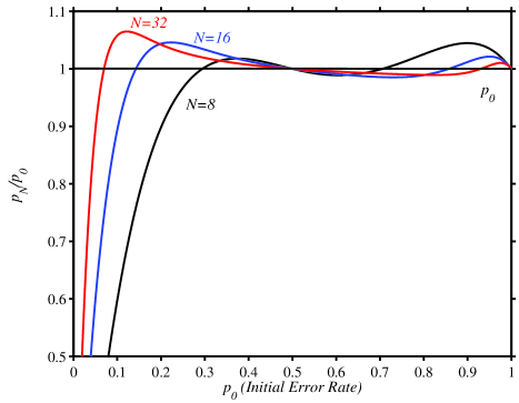
FIG. 1.: The ratio $p_{N}/p_{0}$ for $N=8$, $16$ and $32$. These curves illustrate the change in the probability that a given bit is in error after a single application of Winnow for the indicated block size $N$. Note that $(p_{8}<p_{16})\;{\forall}\;(p_{0}<0.38)$; in addition, $(p_{16}<p_{32})\;{\forall}\;(p_{0}<0.20)$. This indicates that a pplications of Winnow with smaller $N$ are more efficient at removing errors than are applications with larger $N$ within the region where $p_{0}$ satisfies these conditions.

TABLE I.: $\bar{n}_{f}$ for $N=8$ for various stages in Winnow (note that Hamming is not applied to blocks that contain an even number of errors).

$n_{i}$	0	1	2	3	4	5	6	7	8
$\bar{n}_{f}^{p}$	0	0.88	1.75	2.63	3.5	4.38	5.25	6.13	7
$\bar{n}_{f}^{ph}$	0	0	1.75	3.5	3.5	3.5	5.25	7	7
$\bar{n}_{f}$	0	0	1.75	2.0	3.5	2.0	5.25	4	7

TABLE II.: $\bar{n}_{f}/N_{f}$ for $N=8$ for various stages in Winnow (note that the Hamming component of Winnow is not applied to blocks that contain an even number of errors).

$p_{i}$	0	0.13	0.25	0.38	0.5	0.63	0.75	0.88	1
$p_{f}^{p}$	0	0.13	0.25	0.38	0.5	0.63	0.75	0.88	1
$p_{f}^{ph}$	0	0	0.25	0.5	0.5	0.5	0.75	1	1
$p_{f}$	0	0	0.25	0.5	0.5	0.5	0.75	1	1

REFERENCES

- [1] C. H. Bennett and G. Brassard, International Conference on Computers, Systems & Signal Processing, Bangalore, India, 1984 (IEEE, New York, 1984) 175-179; A. K. Ekert, Phys. Rev. Lett. 67, 661-663 (1991); C. H. Bennett and S. J. Wiesner, Phys. Rev. Lett. 69, 2881-2884 (1992); C. H. Bennett, Phys. Rev. Lett. 68, 3121-3124 (1992).
- [2] C. Cachin and U. M. Maurer, J. Cryptology 10, 97-110 (1997).
- [3] N. Ltkenhaus, Phys. Rev. A 59, 3301-3319 (1999).
- [4] C. H. Bennett et al., Lect. Notes in Comput. Sci. 473, 253-265 (1990); J. of Cryptology 5, 3-28 (1992).
- [5] G. Brassard and L. Salvail, Lect. Notes Comput. Sci. 765, 410-423 (1994).
- [6] C. H. Bennett et al., IEEE Trans. Inf. Theory 41, 1915-1923 (1995).
- [7] W. Diffe and M. E. Hellman, Proceedings of AFIPS National Computer Conference, 109-112 (1976); R. L. Rivest, A. Shamir and L. M. Adleman, Communications of the ACM 21, 120-126 (1978); C. Mitchell, F. Piper and P. Wild, G. J. Simmons (Ed.), Contemporary Cryptography: The Science of Information Integrity, 325-378 IEEE Press, 1992.
- [8] R. W. Hamming, The Bell System Technical Journal 2, 147-161 (1950).
- [9] R. W. Hamming, Coding and Information Theory, Prentice Hall, 239 pp, New Jersey (1986,1980).
- [10] C. E. Shannon, The Bell System Technical Journal 27, 379-423 and 623-656 (1948).
- [11] A. J. Menezes, P. C. van Oorschot and S. A. Vanstone, Handbook of Applied Cryptography, 780 pp, CRC Press, New York (1997).
- [12] M. Duek, O. Haderka and M. Hendrych, Opt. Commun. 169, 103-108 (1999).
- [13] J. Kim et al., Nature 397 500-503 (1999); P. Michler et al., Science 290, 2282 (2000); B. Lounis and W. E. Moerner, Nature 407, 491 (2000).
- [14] J. D. Franson and H. Ives, Appl. Opt. 33, 2949-2954 (1994); B. Jacobs and J. D. Franson, Opt. Lett. 21, 1854-1856 (1996); P. D. Townsend, Nature 385, 47-49 (1997); A. Muller, H. Zbinden and N. Gisin, Europhys. Lett. 33, 335-339 (1996); W. T. Buttler et al., Phys. Rev. Lett. 84, 5652-5655 (2000); R. J. Hughes, G. L. Morgan and C. Glen Peterson, J. Mod. Opt. 47, 533-547 (2000); D. S. Bethune and W. P. Risk, IEEE J. Quant. Elect. 36, 340-347 (2000); M. Bourennane et al., J. Mod. Opt. 47, 563-579 (2000); J. G. Rarity, P. R. Tapster and P. M. Gorman, J. Mod. Opt. 48, 1887-1901 (2001).