Experimental Investigation of the Robustness of Partially Entangled Photons over 11km

Abstract

We experimentally investigate the robustness of maximal and non-maximal Time-Bin entangled photons over distances up to 11 km. The entanglement is determined by controllable parameters and in all cases is shown to be robust, in that the photons maintain their degree of entanglement after transmission.

Quantum communication and quantum networks are only part of a much larger field now of Quantum Information Science Nielsen00a . At the heart of many of these associated endeavours is entanglement Tittel01a . Entangled states also play an essential role with respect to the fundamental nature of the microscopic world as investigated in tests of Bell inequalities Einstein35 ; Bell64 ; Aspect82 ; Tittel98 ; Weihs98 . Beyond the mere existence of entanglement, quantum communication schemes like quantum cryptography Eckert91 ; Gisin02a and teleportation Bennett93a ; Bouwmeester97a ; Rome98a ; Shih01a have been developed to utilise what has become known as this quantum resource, entanglement. Schemes using photonic quantum channels that connect distant nodes of a quantum network Cirac97a or for quantum repeaters Breigel98a rely on the possibility to broadcast entanglement over significant distances.

An important aspect which has received little attention from an experimental perspective is that information may need to be encoded in possibly unknown states of arbitrary degrees of entanglement. At a fundamental level, we expect that the entanglement should be robust whether the state is maximally entangled or not. Depending on the decohering environment this may not be the case. At some intuitive level however, we may be inclined to believe that due to their inherent symmetry, maximally entangled states are more robust against decoherence than non-maximal ones. We will consider a state to be robust if, when it is detected, the initial entanglement is unchanged over the length of the transmission.

We have previously shown that maximally entangled Energy-Time photons are robust enough to violate a Bell inequality between analysers 10 km apart Tittel98 . In this letter, we now investigate the robustness of partially, and maximally, entangled Time-Bin Qubits, when transmitted over long optical fibers, along the way providing the necessary basis for distribution of arbitrary states.

Entangled time-bin photons (entangled qubits) Brendel99a can be created using the experimental setup pictured in Fig.(1). A coherent superposition of two classical pump pulses is generated, from a single diode laser pulse, after passing through a Bulk optics Michelson interferometer with a large path-length difference. The laser produces pulses of less than 100 ps width at a frequency of 80 MHz with a wavelength of 657 nm. In this scheme the pulse duration must be short compared to the travel time difference of the pump interferometer, 1.2 ns in our case. The two pulses then undergo spontaneous parametric downconversion in a Periodically Poled Lithium-Niobate (PPLN) waveguide Tanzilli01a ; Tanzilli01b producing pairs of entangled photon at 1314 nm wavelength, convenient for fibre telecommunication. At these wavelengths the detection is obtained via passively quenched germanium avalanche photodiodes, operated in Geiger mode and cooled to 77 K. Depending on the amplitudes of the two classical pulses and the relative phase, one can create maximally and non-maximally entangled states of the form

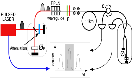
Figure 1: Experimental schematic: A pulsed laser diode source and Michelson interferometer produce 2 pump pulses which are then incident on a PPLN waveguide producing 2 entangled photons. After filtering (F), each pair is collected and transmitted along a fibre spool to a fibre Michelson interferometer. A circulator (C) allows input and detection on the same port. A triple coincidence between 2 photons and one of the pump pulses then detects the entangled state.

$$|\psi\rangle=\alpha|1,0;1,0\rangle_{AB}+\beta e^{i\phi_{P}}|0,1;0,1\rangle_{AB}$$ (1)

where $\alpha$ and $\beta$ are real and $\alpha^{2}+\beta^{2}=1$, due to normalisation. Our notation represents, in the case of a state like $|n,0;0,m\rangle$, that $n$ photons are in the first time-bin for $A$ and that $m$ photons are in the second time-bin for $B$. The time difference is obtained as a result of the photons having taken either the short or long arms of the Bulk, or ”Pump”, interferometer, and $\phi_{P}$ is the resulting relative phase. For equal amplitudes, $\alpha=\beta$, the state is maximally entangled, and when $\phi_{P}$=0, Eq.(1) corresponds to the maximally entangled Bell state $|\phi^{+}\rangle$.

After passing through the second (fibre) interferometer the state can be described by:

$$|\psi^{\prime}\rangle=\alpha|1,0,0;1,0,0\rangle_{AB}+\alpha e^{2i\phi_{I}}|0,1,0;0,1,0\rangle_{AB}$$

$$+\beta e^{i\phi_{P}}|0,1,0;0,1,0\rangle_{AB}+\beta e^{i(2\phi_{I}-\phi_{P})}|0,0,1;0,0,1\rangle_{AB}.$$ (2)

The resulting double coincidences for the pump and A (and the pump and B) from this state correspond to the three peaks of the coincidence histogram, as depicted at the bottom of Fig.(1). The two middle terms of this state interfere with respect to the amplitudes and phases of our initial entangled state in the central time bin. We can distinguish the first and last terms in Eq.(2) via the pump timing information. Thus, conditioning the detection on events in both middle peaks by making a triple coincidence corresponds to a projective measurement onto the state of Eq.(1).

In this experiment we are not concerned with questions of non-locality but simply with the robustness of the Time-Bin entangled states. As such we primarily utilise a ”Franson Replié” arrangement which utilises only one analyser interferometer as depicted in Fig.(1). This arrangement can be thought of as having used the symmetry of the standard Franson interferometer setup Franson89a and folded it in half so both interferometers were on top of each other in a sense. After the 11 km of fibre (on a spool) a circulator is placed at one port of the interferometer allowing us to both input and detect. The other detector operates normally on the other port. Coincidences correspond to both photons taking the short or the long paths together as opposed to doing it in independent interferometers. Whilst we believe that the correlations will be the same, whether we use one or two interferometers, we will give some results with respect to an experimental arrangement with two interferometers so that each photon travels over an independent 2.4 km length of fibre. This is done by placing a 2x2 fibre coupler (beamsplitter) after the PPLN waveguide in Fig.(1), connected to the two fibres, each with an interferometer, where detection is made on one output of each.

During transmission these pure states can in general suffer from environment induced phase as well as from bit flips. Bit flips can happen if the broadening of the photon (in time space), due to chromatic dispersion effects in fibers, is such that the amplitude initially located in one time bin starts overlapping with the one in the other time bin. ie the three peaks at the bottom of Fig.(1) merge together. This reduces our ability to discriminate between them, and hence we loose information. This can be prevented in several ways: we already produce our entangled photons centered at telecommunication wavelength of 1.3 $\mu$m where chromatic dispersion is zero, thus reducing the susceptibility to dispersion. We can improve this non-locally by using the right choice of wavelength determined by the dispersion curve of the fibers, in the same way that it is done for energy-time entangled states Franson92a ; Tittel99a . However, note that the compensation will be less perfect as the energy correlation between the entangled qubits is less stringent. Further on, we can utilise interference filters, in our case of 40 nm width, to reduce the spectral width of the photons, leading to a less pronounced spread of the pulse during a given transmission distance. And finally, we can increase the separation between the time bins, but this would make the interferometers larger and less stable and render the qubits more vulnerable to phase errors during transmission.

Phase errors generally arise as a result of some random variation between the two time bins but this is negligible in our case, at least as far as transmission is concerned. With 1.2 ns separation between time bins there would need to be very high (GHz) frequency noise in order to produce a phase flip. Our main phase error arises during creation and detection of ensembles of photons over extended periods of time. This requires that the interferometers have the same path-length difference for the entire time that we prepare and measure a particular state. This will be discussed further as we discuss our states.

If we are going to generate non-maximally entangled states, then an important question is: how can we characterise them? Firstly we can restrict our attention to pure states of the form of Eq.(1), as we post-select the final state. Now, given the state in Eq.(2), the probability of coincidence in the central time-bin is given by,

$$P_{c}=0.5[\alpha^{2}+\beta^{2}+2\alpha\beta cos(\phi)].$$ (3)

We see that the probability of a coincidence detection varies with the phase, $\phi=2\phi_{I}-\phi_{P}$. Therefore, by varying the phase, we can scan through maximum and minimum probabilities corresponding to regimes of maximum constructive and destructive interference and thus determine the Visibility which is given by,

$$V=2\alpha\beta.$$ (4)

Our fibre interferometers are thermally stabilised and the phase is varied by changing the temperature of the interferometer.

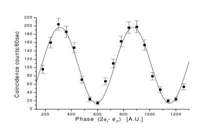
Figure 2: The nett Interference fringes for the experimental setup shown in Fig.(1) after the photons had travelled 11 km.

In Fig.(2) we see the results of this approach using the experimental setup in Fig.(1) with 11 km of fibre. Depicted are the nett count rates after subtraction of accidental coincidences. We will comment on this later. Due to the long distances the signal is reduced and hence we have to count for a longer time, 60 seconds in this instance. The squares denote the number of triple coincidences in each 60 second interval. It is for this 60 second integration time that we have to maintain the stability of the laser to within a fraction of a wavelength to minimise the phase errors discussed previously. The solid line that traces these points is a sinusoidal fit to the data derived from Eq.(3) and allows us to determine the Visibility.

The key here is that the nett Visibility parameterises the entanglement in the final state, as we would expect. Both the bit-flips and phase flips will manifest themselves as a reduction in Visibility and as such we will use this as the experimental measure of our entanglement. With respect to Fig.(2), this analysis returns a value of $V=94.2\pm 4.8\%$ after transmitting the maximally entangled state over 11km. The error in this result, $\Delta V$, is determined by the numerical uncertainty in the sinusoidal fit to the data.

Table(1) shows the raw Visibility as well as the nett Visibility, which is derived after subtracting the accidental coincidences, for maximally entangled states with both one and two interferometers. We see that although the raw Visibility is less over the longer distances, the nett Visibilities are almost equivalent.

Run	Distance	$V_{raw}\hskip 11.38109pt$	$V_{nett}\hskip 11.38109pt$	$\Delta V\hskip 11.38109pt$
I	0 km	90.2	94.9	3.7
II	11 km	86.8	94.2	4.8
III	0 km	89.1	92.7	4.7
IV	2.4 km	84.5	92.2	4.8

Table 1: The raw and nett (accidental coincidences subtracted) Visibilities for the maximally entangled states. I and II use 1 interferometer and rows III and IV use 2. $\Delta V$ is the uncertainty in the Visibility.

Let us briefly comment on the nature of accidental coincidences. They occur if both events in the coincidence window are triggered by noise. Also, there will be contributions if one photon triggers one detector and noise triggers the other while the photon’s correlated partner is absorbed in the fiber. Thus, the resulting decrease of raw visibility is due to a combination of fiber losses and detector noise. However, since we are interested in the impact of bit and phase flips on the entanglement, we must subtract this source of noise which is well understood and is easily measured.

The other aspect of characterisation is related to generating the non-maximally entangled states. We can quantify the expected entanglement in the state in terms of the Entropy of Entanglement:

$$E=-\alpha^{2}log_{2}\alpha^{2}-(1-\alpha^{2})log_{2}(1-\alpha^{2}),$$ (5)

where we use the amplitudes of the two pump pulses, appropriately normalised. With this experimental setup non-maximally entangled states can be realised in a controlled manner by varying the attenuation in one of the arms of the pump interferometer so that the classical pulses have unequal magnitudes. In practice we vary the attenuation in both arms so that we have the same mean power before the waveguide.

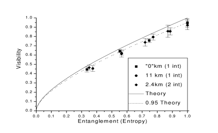
Figure 3: Nett Visibility of the output state as a function of the expected Entanglement, measured at our source. The relationship is unchanged by transmission over significant distances.

The results of the measurements of the non-maximally entangled states are given in Fig.(3). The solid line shows the theoretically expected Visibility from Eq.(4) as a function of the Entanglement Eq.(5) as $\alpha$ and $\beta$ are varied. In the experiment we have complete control over the classical amplitudes and these are measured directly at the output of the pump interferometer. After transmission the nett Visibility are obtained from sinusoidal fits described previously. On average, subtraction of the noise improved the raw Visibilities for the 0 distance runs by less than 5% and the 11 km runs by less than 9%. A dashed line corresponding to the theory but scaled to have a maximum Visibility of 95% is also shown. We see that for both the experimental setup as depicted in Fig.(1), with or without 11 km of fibre, and also with one or with two interferometers the results are in good agreement with the theory. Specifically we see that regardless of the initial entanglement or the distance travelled that there is no loss of entanglement over transmission for any of the states.

With our experimental configuration we don’t have access to an absolute phase reference within the system and hence standard tomographic techniques White99a ; James01a ; Thew02a won’t work. Given that the entanglement could be parameterised by the Visibility and there were no adverse effects due to decoherence, there appears little to be gained by reconstructing the full density matrix for the state.

In this experiment we use a PPLN waveguide which provides a highly efficient generator of entangled photons. A consequence of this high efficiency, conversion rates 4 orders of magnitude higher than obtained with bulk sources Tanzilli01a ; Tanzilli01b , is that when using a pulsed laser the probability of producing multiple photon pairs per pulse can become significant. This has the effect of reducing the Interference Visibility and hence at a more fundamental level the entanglement. This is a critical point especially in experiments of this nature. We ensured that we had the same mean power at the PPLN waveguide throughout these experiments. This was done so that any reduction in the Visibilility was due to decoherence and not due to variation in the rate of production of photon pairs.

A theory describing this behaviour has recently been developed, the details of which will be presented elsewhere Marcikic02a . From this we expect the Visibility to be related inversely to the number of photon pairs produced, $V=1/n$. If we also make the assumption that the pairs satisfy a Poissonian distribution, where $P(n)=\mu^{n}e^{-\mu}/n!$ is the probability of having $n$ pairs and $\mu$ is the mean number of photon pairs created per pulse, then we can find the following relationship

$$V(\mu)=V_{max}\frac{e^{-\mu}}{1-e^{-\mu}}\sum_{n\geq 1}\frac{\mu^{n}}{n!n}.$$ (6)

Here $V_{max}$ is a scaling factor to compensate for known factors that reduce the Visibility in a given experiment. From our knowledge of the experimental setup we can relate the measured quantities, the 2 single photon count rates, $S_{1},S_{2}$, and the average coincidence count rate, $R_{c}$, to give us an estimate of the mean number of photon pairs, $\mu_{e}=S_{1}S_{2}/4R_{c}f$, where $f$ is the frequency of the pulsed laser source. This gives us a measure that not only takes account of collection and detection efficiencies but also losses, which is convenient when working over long distances. We see in Fig.(4) that theory and experiment are in good agreement which allowed us to optimise the power so as to efficiently generate arbitrarily entangled states for transmission.

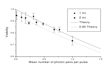
Figure 4: Interference Visibility as a function of the mean number of Photon Pairs in each pulse of the laser.

We have shown that we can generate, in a controlled way, states with arbitrary degrees of entanglement using a pulsed diode laser and a PPLN waveguide. This is very much a new technology under development which holds great promise for integrated quantum optics and hence quantum communication. The main results proved resoundingly that Time-Bin entanglement is robust with transmission distances up to 11 km.

This work was supported by the Swiss NCCR ”Quantum Photonics” and the European QuComm IST projects. W.T. acknowledges funding by the ESF Programme Quantum Information Theory and Quantum Computation (QIT)

References

- (1) See for instance, M. A. Nielsen and I. L. Chuang, Quantum Computation and Quantum Information, Cambridge University Press, Cambridge, (2001)
- (2) W. Tittel, and G. Weihs, Quantum Inf. and Comp., 1, No.2, 3 (2001)
- (3) A. Einstein, B. Podolski and N. Rosen, Phys. Rev. Lett., 47, 1215 (1935)
- (4) J. S. Bell, Speakable and Unspeakable in Quantum Mechanics, Cambridge University Press, Cambridge, (1987)
- (5) A. Aspect, J. Dalibard, and G. Roger, Phys. Rev. Lett., 49, 1804 (1982)
- (6) W. Tittel et al., Phys. Rev. A, 81 , 3563 (1998)
- (7) G. Weihs et al., Phys. Rev. Lett., 81, 5039 (1998)
- (8) A. Ekert, Phys. Rev. Lett., 67, 661 (1991)
- (9) N. Gisin et al., Rev. Mod. Phys., 74, 145 (2002)
- (10) C. H. Bennett et al., Phys. Rev. Lett., 70, 1895 (1993)
- (11) D. Bouwmeester et al., Nature, 390, 575 (1997)
- (12) D. Boschi et al., Phys. Rev. Lett. 80 1121 (1998)
- (13) Y. Kim, S. P. Kulik, and Y. Shih, Phys. Rev. Lett., 86, 1370 (2001)
- (14) J. Cirac et al., Phys. Rev. Lett., 78, 3221 (1997)
- (15) H. J. Briegel et al., Phys. Rev. Lett., 81, 5932 (1998)
- (16) J. Brendel et al., Phys. Rev. Lett., 82, 2594 (1998)
- (17) S. Tanzilli et al., Elect. Lett., 37, 28 (2001)
- (18) S. Tanzilli et al., Eur. Phys. J. D, 18, 155 (2002).
- (19) A. G. White et al., Phys. Rev. Lett., 83, 3101 (1999).
- (20) D. F. V. James et al., Phys. Rev. A., 64, 052312 (2001).
- (21) R. T. Thew et al., quant-ph/0201052 (2002)
- (22) J. D. Franson, Phys. Rev. Lett., 62, 2205 (1989)
- (23) J. D. Franson, Phys. Rev. A, 45, 3126 (1992)
- (24) W. Tittel et al., Phys. Rev. A, 59, 4150 (1999)
- (25) I. Marcikic, In preparation. (2002)