Temporal Interferometry: A Mechanism for Controlling Qubit Transitions During Twisted Rapid Passage with Possible Application to Quantum Computing

Abstract

In an adiabatic rapid passage experiment, the Bloch vector of a two-level system (qubit) is inverted by slowly inverting an external field to which it is coupled, and along which it is initially aligned. In twisted rapid passage, the external field is allowed to twist around its initial direction with azimuthal angle $\phi(t)$ at the same time that it is inverted. For polynomial twist: $\phi(t)\sim Bt^{n}$. We show that for $n\geq 3$, multiple avoided crossings can occur during the inversion of the external field, and that these crossings give rise to strong interference effects in the qubit transition probability. The transition probability is found to be a function of the twist strength $B$, which can be used to control the time-separation of the avoided crossings, and hence the character of the interference. Constructive and destructive interference are possible. The interference effects are a consequence of the temporal phase coherence of the wavefunction. The ability to vary this coherence by varying the temporal separation of the avoided crossings renders twisted rapid passage with adjustable twist strength into a temporal interferometer through which qubit transitions can be greatly enhanced or suppressed. Possible application of this interference mechanism to construction of fast fault-tolerant quantum CNOT and NOT gates is discussed.

I Introduction

Adiabatic rapid passage (ARP) is a well-known procedure for inverting the Bloch vector of a two-level system (qubit) arp . This is accomplished by inverting an external field $\mathbf{F}(t)$ which couples to the qubit, and along which the qubit is initially aligned. The field inversion is done on a time-scale that is large compared to the inverse Rabi frequency $\omega_{0}^{-1}$ (viz. adiabatic), though small compared to the thermal relaxation time $\tau$ (viz. rapid). In the usual case, $\mathbf{F}(t)$ remains within a plane that includes the origin: $\mathbf{F}(t)=b\,\hat{\mathbf{x}}+at\,\hat{\mathbf{z}}$, with $-T_{0}/2<t<T_{0}/2$, and $\omega_{0}^{-1}\ll T_{0}\ll\tau$.

ARP can be used to implement a NOT gate on the quantum state of a qubit. If one identifies the computational basis states $|0\rangle$ and $|1\rangle$, respectively, with the spin-up and spin-down eigenstates along the initial direction of the external field $\mathbf{F}(-T_{0}/2)$, then ARP maps $|0\rangle\leftrightarrow|1\rangle$ which is the defining operation of a NOT gate. Occurrence of a transition during ARP corresponds to an error in the NOT gate since the Bloch vector is not inverted, and thus $|i\rangle\rightarrow|i\rangle$, ($i=0,1$). Thus we can identify the ARP transition probability with the NOT gate error probability. For ARP, the adiabatic nature of the inversion ensures that the error probability is exponentially small. The price paid for this reliability, however, is an extremely slow NOT gate.

In twisted adiabatic rapid passage, the external field is allowed to twist around its initial direction with azimuthal angle $\phi(t)$ at the same time that it is adiabatically inverted: $\mathbf{F}(t)=b\cos\phi(t)\,\hat{\mathbf{x}}+b\sin\phi(t)\,\hat{\mathbf{y}}+at\,\hat{\mathbf{z}}$. Reference bry, showed that for twisted ARP, the exponentially small transition probability contains a factor $\exp[\,\Gamma_{g}\,]$ of purely geometric origin. The simplest case where $\Gamma_{g}\neq 0$ corresponds to quadratic twist: $\phi(t)=Bt^{2}$. Zwanziger et. al. zwa were able to experimentally realize ARP with quadratic twist and obtained results in agreement with the predictions of Reference bry, .

In this paper we will consider twisted rapid passage with polynomial twist, $\phi(t)\sim Bt^{n}$, and we will focus exclusively on qubit inversions done at non-adiabatic rates. Although we will briefly consider quadratic twist in Section II as a test case for our numerical simulations, our interest will not be the geometric effect of Reference bry, . Instead, our primary focus will be on establishing the existence of multiple avoided crossings during twisted rapid passage when $n\geq 3$, and with exploring some of their consequences. After general considerations (Section II), we will explicitly examine cubic ($n=3$) and quartic ($n=4$) twist, and will provide clear evidence that the multiple avoided crossings produce strong interference effects in the qubit transition probability. The transition probability is shown to be a function of the twist strength $B$, which can be used to control the time-separation of the avoided crossings, and hence the character of the interference (constructive or destructive). Cubic and quartic twist are examined in Sections III and IV, respectively. We shall see that interference between the multiple avoided crossings can greatly enhance or suppress qubit transitions. The interference effects are a direct consequence of the temporal phase coherence of the wavefunction. The ability to vary this coherence by varying the temporal separation of the avoided crossings renders twisted rapid passage with adjustable twist strength into a temporal interferometer through which qubit transitions can be controlled. It will be shown that quartic twist can implement qubit inversion non-adiabatically while operating at a fidelity that exceeds the threshold for fault tolerant operation. Finally, in Section V, we summarize our results and discuss possible application of this interference mechanism to quantum computing. In particular, we describe how one might use non-adiabatic rapid passage with quartic twist to construct a fast fault-tolerant quantum CNOT gate.

It is worth noting that experimental confirmation of the work described in this paper has recently been carried out by Zwanziger et. al. jwz . They have realized non-adiabatic rapid passage with both cubic and quartic twist, and have observed clear evidence of constructive and destructive interference in the qubit transition probability due to interference between the avoided crossings, with excellent agreement between the experimental data and our numerical simulations. This experimental work provides clear proof-of-principle for our thesis that controllable quantum interference exists during twisted rapid passage. With this thesis now experimentally confirmed, future research can focus on applying this interference to the task of constructing fast fault tolerant quantum CNOT and NOT gates.

After this paper was submitted, previous work was brought to our attention which also examined models of rapid passage in which more than one avoided crossing is possible, and in which interference effects were also considered lim ; suo ; joy . These papers focused solely on the adiabatic limit. Application of this adiabatic theory to the Zwanziger experiment yields predictions that are in poor agreement with the experimental results jwz . This failing is no doubt a consequence of the non-adiabatic character of this experiment whose results thus lies beyond the scope of the adiabatic theory developed in these papers. In contrast, the work we present below is principally interested in the non-adiabatic limit, and our simulation results are in full agreement with experiment jwz . We also consider possible application of these interference effects to the construction of fast fault-tolerant quantum CNOT and NOT gates. Ref. lim ; suo ; joy do not consider such applications.

II Twisted Rapid Passage

We begin by briefly summarizing the essential features of rapid passage in the absence of twist. Twistless rapid passage describes a wide variety of phenomena, ranging from magnetization reversal in NMR, to electronic transition during a slow atomic collision. The essential situation is that of a qubit which is Zeeman-coupled to a background field $\mathbf{F}(t)$,

$$H(t)=\mbox{\boldmath$\sigma$}\cdot\mathbf{F}(t)=\left(\begin{array}[]{cc}at&b\\ b&-at\end{array}\right)\hskip 7.22743pt,$$ (1)

with $\mathbf{F}(t)=b\,\hat{\mathbf{x}}+at\,\hat{\mathbf{z}}$. This particular form for $\mathbf{F}(t)$ describes inversion of the background field in such a way that it remains in the x-z plane throughout the inversion. For simplicity, we assume $a,\>b>0$ throughout this paper. The instantaneous energies $E_{\pm}(t)$ are:

$$E_{\pm}(t)=\pm\sqrt{b^{2}+(at)^{2}}\hskip 7.22743pt,$$ (2)

and an avoided crossing is seen to occur at $t=0$ where the energy gap is minimum. The Schrodinger dynamics for twistless rapid passage can be solved exactly for arbitrary values of $a$ and $b$ lan ; zen , and yields the Landau-Zener expression for the transition probability $P_{LZ}$:

$$P_{LZ}=\exp\left[\,-\frac{\pi b^{2}}{\hbar|a|}\,\right]\hskip 7.22743pt.$$ (3)

II.1 Twisted Rapid Passage and Multiple Avoided Crossings

In twisted rapid passage, the background field $\mathbf{F}(t)$ is allowed to twist around its initial direction during the course of its inversion: $\mathbf{F}(t)=b\cos\phi(t)\,\hat{\mathbf{x}}+b\sin\phi(t)\,\hat{\mathbf{y}}+at\,\hat{\mathbf{z}}$. It proves convenient to transform to the rotating frame in which the x-y component of the background field is instantaneously at rest. This is accomplished via the unitary transformation $U(t)=\exp[-(i/2)\phi(t)\sigma_{z}]$. The Hamiltonian $\overline{H}(t)$ in this frame is:

$$\overline{H}(t)=\mbox{\boldmath$\sigma$}\cdot\overline{\mathbf{F}}=\left(\begin{array}[]{cc}\left(\,at-\frac{\hbar}{2}\dot{\phi}\,\right)&b\\ b&-\left(\,at-\frac{\hbar}{2}\dot{\phi}\,\right)\end{array}\right)\hskip 7.22743pt,$$ (4)

where $\overline{\mathbf{F}}(t)=b\,\hat{\mathbf{x}}+(at-\hbar\dot{\phi}/2)\,\hat{\mathbf{z}}$ is the background field as seen in the rotating frame, and a dot over a symbol represents the time derivative of that symbol. The instantaneous energy eigenvalues are $\overline{E}_{\pm}(t)=\pm\sqrt{\left(\,at-(\,\hbar\dot{\phi}\,)/2\,\right)^{2}+b^{2}}$. Avoided crossings occur when the energy gap is minimum, corresponding to when

$$at-\frac{\hbar}{2}\,\frac{d\phi}{dt}=0\hskip 7.22743pt.$$ (5)

For polynomial twist: $\phi_{n}(t)=c_{n}Bt^{n}$, where $B$ is the twist strength. The dimensionless constant $c_{n}$ has been introduced to simplify some of the formulas below. For later convenience, we chose $c_{n}=2/n$. For polynomial twist, it is easily checked that eqn. (5) always has the root:

$$t=0\hskip 7.22743pt,$$ (6)

and that for $n\geq 3$, eqn. (5) also has the $n-2$ roots:

$$t=\left(\,{\rm sgn}\,B\,\right)^{\frac{1}{n-2}}\,\left(\,\frac{a}{\hbar|B|}\,\right)^{\frac{1}{n-2}}\hskip 7.22743pt.$$ (7)

All together, equation (5) has $n-1$ roots, though only the real roots correspond to avoided crossings. For quadratic twist ($n=2$), only eqn. (6) arises. Thus, for this case, only the avoided crossing at $t=0$ is possible. For $n\geq 3$, along with the avoided crossing at $t=0$, real solutions to eqn. (7) also occur. The different possibilities for this situation are summarized in Table 1.

Table 1: Classification of regimes under which multiple avoided crossings occur for polynomial twist with $n\geq 3$.

1. $\underline{sgn\,B=+1}$
(a)      $n$ odd;	$\>\>\>2$ avoided crossings at:	$\>\>\>t=0$ and $t=\left(a/\hbar B\right)^{1/(n-2)}$
(b)      $n$ even;	$\>\>\>3$ avoided crossings at:	$\>\>\>t=0$ and $t=\pm\left(a/\hbar B\right)^{1/(n-2)}$
2. $\underline{sgn\,B=-1}$
(a)      $n$ odd;	$\>\>\>2$ avoided crossings at:	$\>\>\>t=0$ and $t=-\left(a/\hbar|B|\right)^{1/(n-2)}$
(b)      $n$ even;	$\>\>\>1$ avoided crossing at:	$\>\>\>t=0$

We see that for polynomial twist with $n\geq 3$, multiple avoided crossings always occur for positive twist strength $B$, while for negative twist strength, multiple avoided crossings only occur when $n$ is odd. Note that the time separating the multiple avoided crossings can be adjusted by variation of the twist strength $B$ and/or the inversion rate $a$.

II.2 Brief Detour: Background on Quadratic Twist

As mentioned earlier, quadratic twist has already been examined in the literature bry . It is of interest here only because its dynamics can be solved exactly, and thus allows us to test our numerical simulations before proceeding to unexplored cases of twisted rapid passage. For quadratic twist, $\dot{\phi}_{2}=2Bt$. Inserting this into eqn. (4) gives $\overline{\mathbf{F}}(t)=b\,\hat{\mathbf{x}}+\overline{a}t\,\hat{\mathbf{z}}$, with $\overline{a}=a-\hbar|B|\,(\mathrm{sgn}\,B)$. Thus rapid passage with quadratic twist maps onto twistless rapid passage with $a\rightarrow\overline{a}$. This allows us to obtain an exact result for the transition probability $P_{2}$ for arbitrary values of $a$ and $b$ from eqn. (3) with $a\rightarrow\overline{a}$:

$$P_{2}=\exp\left[\,-\frac{\pi b^{2}}{\hbar|\,a-\hbar|B|\,(\mathrm{sgn}\,B)\,|}\right]\hskip 7.22743pt.$$ (8)

In the adiabatic limit, this reduces to $P_{2}=P_{LZ}\exp[\Gamma_{g}]$, where $\Gamma_{g}=-\pi Bb^{2}/a^{2}$ is the geometric exponent discovered in Ref. bry . Eqn. (8) makes the interesting prediction that a complete quenching of transitions will occur when $\mathrm{sgn}\,B=+1$ and $a=\hbar B$, while no such quenching is possible for $\mathrm{sgn}\,B=-1$. Zwanziger et. al. zwa were able to realize rapid passage with quadratic twist experimentally and confirmed the existence of $\Gamma_{g}$, and the twist-dependent quenching of transitions. We now show that our numerical simulation also reproduces these effects.

II.3 Simulation Details

The equations that drive the numerical simulation follow from the Schrodinger equation in the non-rotating frame:

$$i\hbar\frac{\partial}{\partial t}\,|\psi\rangle=H(t)\,|\psi\rangle\hskip 7.22743pt,$$ (9)

where $H(t)=\mbox{\boldmath$\sigma$}\cdot\mathbf{F}(t)$, and $\mathbf{F}(t)=b\cos\phi(t)\,\hat{\mathbf{x}}+b\sin\phi(t)\,\hat{\mathbf{y}}+at\,\hat{\mathbf{z}}$. To obtain these equations in the adiabatic representation, we expand $|\psi(t)\rangle$ in the instantaneous eigenstates $|E_{\pm}(t)\rangle$ of $H(t)$:

$$|\psi(t)\rangle=S(t)\;e^{-\frac{i}{\hbar}\int_{-T_{0}/2}^{t}\,d\theta\,\left(E_{-}-\hbar\dot{\gamma}_{-}\right)}\;|E_{-}(t)\rangle\;-\;I(t)\;e^{-\frac{i}{\hbar}\int_{-T_{0}/2}^{t}\,d\theta\,\left(E_{+}-\hbar\dot{\gamma}_{+}\right)}\;|E_{+}(t)\rangle\hskip 7.22743pt.$$ (10)

Here $\gamma_{\pm}(t)$ are the geometric phases geo associated with the energy-levels $E_{\pm}(t)$, respectively, and

$$\dot{\gamma}_{\pm}(t)=i\langle\,E_{\pm}(t)\,|\,\frac{d}{dt}\,|\,E_{\pm}(t)\,\rangle=i\langle\,E_{\pm}(t)\,|\,\dot{E}_{\pm}(t)\,\rangle\hskip 7.22743pt.$$ (11)

Substituting eqn. (10) into (9), and using the orthonormality of the instantaneous eigenstates, one obtains the equations of motion for the expansion coefficients $S(t)$ and $I(t)$:

$$\frac{dS}{dt} = -\Gamma^{\ast}(t)\;e^{-i\int_{-T_{0}/2}^{t}\,d\theta\,\delta(\theta)}\;\vspace{0.15in}I(t)\hskip 7.22743pt,$$ (12a)

$$\frac{dI}{dt} = \mbox{}\;\;\;\Gamma(t)\;e^{i\int_{-T_{0}/2}^{t}\,d\theta\,\delta(\theta)}\;S(t)\hskip 7.22743pt.$$ (12b)

Here,

$$\delta(t) = \frac{E_{+}(t)-E_{-}(t)}{\hbar}-\left(\,\dot{\gamma}_{+}(t)-\dot{\gamma}_{-}(t)\,\right)\hskip 7.22743pt,$$ (13)

$$\Gamma(t) = \langle\,E_{+}(t)\,|\,\dot{E}_{-}(t)\,\rangle\hskip 7.22743pt,$$ (14)

and one can show that $\Gamma^{\ast}(t)=-\,\langle E_{-}(t)\,|\,\dot{E}_{+}(t)\,\rangle$. Eqns. (12) are the qubit equations of motion in the adiabatic representation and include the influence of the geometric phase on the dynamics through $\delta(t)$. In the case of twistless rapid passage, the geometric phase vanishes, and eqns. (12) reduce to the well-known equations of motion for a two-level system found in Ref. thr . Eqns. (12) can be put in dimensionless form if we introduce the dimensionless variables: $\tau=(a/b)t$, $\overline{\Gamma}=(b/a)\Gamma$, and $\overline{\delta}=(b/a)\delta$. Here $a$ and $b$ are the parameters that appear in the background field $\mathbf{F}(t)$. One obtains:

$$\frac{dS}{d\tau} = -\overline{\Gamma}^{\ast}\;e^{-i\int_{-\tau_{0}/2}^{\tau}\,d\theta\,\overline{\delta}(\theta)}\;I(\tau)\vspace{0.25in}\hskip 7.22743pt,$$ (15a)

$$\frac{dI}{d\tau} = \mbox{}\;\;\;\overline{\Gamma}\,e^{i\int_{-\tau_{0}/2}^{\tau}\,d\theta\,\overline{\delta}(\theta)}\;S(\tau)\hskip 7.22743pt,$$ (15b)

where $\tau_{0}=(a/b)T_{0}$ is the (dimensionless) time over which the qubit evolves. For rapid passage, the qubit is initially in the negative energy level $|E_{-}(-\tau_{0}/2)\,\rangle$. This corresponds to the initial condition:

$$S(-\tau_{0}/2) = 1\hskip 7.22743pt,$$ (16a)

$$I(-\tau_{0}/2) = 0\hskip 7.22743pt.$$ (16b)

Our numerical simulation integrates eqns. (15) over the time-interval $[\,-\tau_{0}/2,\;\tau_{0}/2\,]$ subject to initial condition (16). From this we determine the asymptotic transition probability $P$:

$$P=|I(\tau_{0}/2)|^{2}\hskip 7.22743pt,$$ (17)

for $\tau_{0}\gg 1$. Later, we will need the $\tau$-values corresponding to the avoided crossings. These are determined by rewriting eqns. (6) and (7) in dimensionless form. To this end, we introduce

$$\eta_{\,n}=\frac{\hbar B\,b^{n-2}}{a^{n-1}}\hskip 7.22743pt,$$ (18)

and recalling that $\tau=(a/b)t$, one easily obtains:

$$\tau=0\hskip 7.22743pt,$$ (19)

and

$$\tau=\left(\,sgn\,\eta_{\,n}\,\right)^{\frac{1}{n-2}}\,\left[\,\frac{1}{|\eta_{\,n}|}\,\right]^{\frac{1}{n-2}}\hskip 7.22743pt.$$ (20)

The avoided crossings correspond to $\tau=0$ and also, for $n\geq 3$, the real solutions of eqn. (20).

II.4 Simulation Test Case: Quadratic Twist

For quadratic twist $\phi_{2}(t)=Bt^{2}$. The instantaneous eigenvalues and eigenvectors of $H(t)$ are easily found to be $E_{\pm}(t)=\pm E(t)$, where $E(t)=\sqrt{b^{2}+(at)^{2}}$, and

$$|E_{+}(t)\,\rangle=\left(\begin{array}[]{c}\cos\frac{\theta}{2}\\ \sin\frac{\theta}{2}\,e^{i\phi_{2}}\end{array}\right)\hskip 36.135pt;\hskip 36.135pt|E_{-}(t)\,\rangle=\left(\begin{array}[]{c}\sin\frac{\theta}{2}\\ -\cos\frac{\theta}{2}\,e^{i\phi_{2}}\end{array}\right)\hskip 7.22743pt,$$ (21)

with $\cos\theta=at/E$. From the eigenstates one obtains:

$$\dot{\gamma}_{\pm}(t) = -\frac{\dot{\phi}_{2}}{2}\left(\,1\mp\cos\theta\,\right)\hskip 7.22743pt;$$ (22a)

$$\Gamma(t) = \frac{\dot{\theta}}{2}-i\frac{\dot{\phi}_{2}}{2}\sin\theta\hskip 7.22743pt;$$ (22b)

$$\delta(t) = \frac{2E}{\hbar}-\dot{\phi}_{2}\cos\theta\hskip 7.22743pt.$$ (22c)

$\overline{\Gamma}(\tau)$ and $\overline{\delta}(\tau)$ are then determined from eqns. (22b) and (22c) and are found to depend parametrically on the dimensionless “inversion rate” $\lambda=\hbar a/b^{2}$ and the dimensionless “twist strength” $\eta_{\,2}=\hbar B/a$. “Inversion rate” and “twist strength” are placed in quotes as $\lambda$ does not depend solely on the inversion rate $a$, nor $\eta_{\,2}$ solely on the twist strength $B$. Crudely speaking, $\lambda=1$ can be thought of as the boundary separating adiabatic and non-adiabatic inversion rates, with $\lambda>1$ corresponding to non-adiabatic inversion. Having determined $\overline{\Gamma}(\tau)$ and $\overline{\delta}(\tau)$, eqns. (15) are integrated numerically using an adjustable step-size fourth-order Runge-Kutta algorithm. To simplify comparison of the numerical result for the transition probability with the exact result $P_{2}$, we re-write eqn. (8) in terms of $\lambda$ and $\eta_{\,2}$. One finds:

$$P_{2}=\exp\left[\,-\frac{\pi}{\lambda}\,\frac{1}{\left|\,1-\eta_{\,2}\,\right|}\,\right]\hskip 7.22743pt.$$ (23)

Figure 1 shows a representative plot of the transition probability $P(\tau)=|I(\tau)|^{2}$ versus $\tau$.

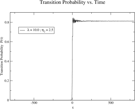
Figure 1: Representative plot of transition probability $P(\tau)$ for quadratic twist with $\lambda=10.0$ and $\eta_{\,2}=2.5$.

It is clear for the Figure that the transition occurs in the vicinity of the avoided crossing at $\tau=0$. Note also that $P(\tau)$ has a small oscillation about its asymptotic value $P=\lim_{\tau\rightarrow\infty}\,P(\tau)$. To average out the oscillation, $P(\tau)$ (for given $\lambda$ and $\eta_{\,2}$) was calculated for 10 different values of $\tau\gg 1$, and $P$ was identified with the average. Figures 2 and 3 show our numerical results for $P$ for various values of $\eta_{\,2}$ for $\lambda=10.0$ and $\lambda=3.0$, respectively. Also plotted in each of these Figures is the exact result $P_{2}$ (eqn. (23)).

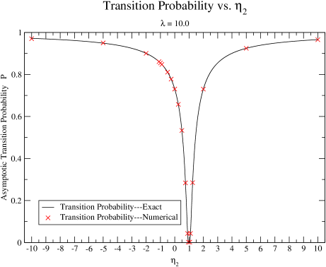
Figure 2: Numerical results for the asymptotic transition probability $P$ versus $\eta_{\,2}$ for quadratic twist with $\lambda=10.0$. Also plotted is the exact result $P_{2}$.

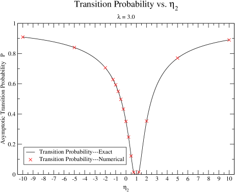
Figure 3: Numerical results for the asymptotic transition probability $P$ versus $\eta_{\,2}$ for quadratic twist with $\lambda=3.0$. Also plotted is the exact result $P_{2}$.

Figures 2 and 3 show that our numerical results are in excellent agreement with the exact result $P_{2}$, and clearly show the quenching of transitions at $\eta_{\,2}=1$, and the absence of quenching for negative $\eta_{\,2}$. The $\lambda$ values shown are purposely highly non-adiabatic. We see that the twist-induced quenching clearly persists into the non-adiabatic regime, although the width of the quench decreases with increasing $\lambda$. The agreement of our simulations with eqn. (23) at small $\eta_{\,2}$ indicates that our simulations also account for the geometric factor $\exp\left[\Gamma_{g}\right]$ in $P_{2}$. Having established that our numerical algorithm correctly reproduces the essential results of rapid passage with quadratic twist, we go on to consider the unexplored areas of rapid passage with higher order twist. Referring to Table 1, we see that all cases with odd $n$ have 2 avoided crossings. Cubic ($n=3$) twist corresponds to the simplest example of odd-order twist, and it is examined in the following Section. Similarly, quartic ($n=4$) twist is the simplest example of even-order twist, and we examine it in Section IV.

III Cubic Twist

Having successfully tested our numerical algorithm against the exact results for quadratic twist, we go on to consider cubic twist for which $\phi_{3}(t)=(2/3)Bt^{3}$, and $\eta_{\,3}=\hbar Bb/a^{2}$ (see eqn. (18)). As in Section II, the instantaneous eigenvalues of $H(t)$ are $E_{\pm}(t)=\pm E(t)$, and the instantaneous eigenstates are given by eqn. (21) with $\phi_{2}(t)\rightarrow\phi_{3}(t)$. Eqns. (22) again apply, however $\dot{\phi}_{2}(t)\rightarrow\dot{\phi}_{3}(t)$, and $\overline{\Gamma}(\tau)$ and $\overline{\delta}(\tau)$ are determined from eqns. (22b) and (22c). Having determined $\overline{\Gamma}(\tau)$ and $\overline{\delta}(\tau)$, eqns. (15) can be numerically integrated subject to the initial condition specified in eqns. (16). Before examining results of that integration, we show in Figure 4 a plot of the numerical results for the transition probability $P(\tau)$ for $\lambda=5.0$ and $\eta_{\,3}=0$.

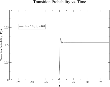
Figure 4: Plot of the transition probability $P(\tau)$ for twistless non-adiabatic rapid passage with $\lambda=5.0$ and $\eta_{\,3}=0$.

This corresponds to twistless non-adiabatic rapid passage, and we include this plot for later comparison with related plots for cubic and quartic twist. The asymptotic transition probability for this case is $P=0.533$. Thus, if we were to use this example of twistless non-adiabatic rapid passage to implement a fast NOT-operation on a qubit, the operation would be slightly more likely to produce an inversion (bit-flip) error than not. We will show below that if a small amount of cubic twist is included, the bit-flip error probability can be reduced by 2 orders of magnitude while still maintaining the non-adiabatic inversion rate $\lambda=5.0$. This substantial reduction in error probability is due to destructive interference between the two avoided crossings that occur during rapid passage with cubic twist.

III.1 Demonstration of Quantum Interference

From eqns. (19) and (20), we see that cubic twist is expected to have 2 avoided crossings at $\tau_{1}=0$ and $\tau_{2}=sgn\,\eta_{\,3}/|\eta_{\,3}|$. Figures 5 and 6 show $P(\tau)$ for $\lambda=5.0$ and $\eta_{\,3}=0.02$ and $\eta_{\,3}=-0.02$, respectively.

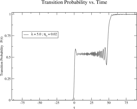
Figure 5: The transition probability $P(\tau)$ for non-adiabatic rapid passage with cubic twist with $\lambda=5.0$ and $\eta_{\,3}=0.02$.

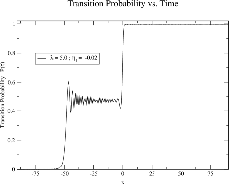
Figure 6: The transition probability $P(\tau)$ for non-adiabatic rapid passage with cubic twist with $\lambda=5.0$ and $\eta_{\,3}=-0.02$.

Figure 5 (6) clearly shows the expected avoided crossings at $\tau=0$ and $\tau=50$ ($-50$). It is also clear from these Figures, and comparison with Figure 4, that the avoided crossings are constructively interfering, leading to an asymptotic transition probability of $P=0.997$. Figures 7 and 8 show $P(\tau)$ for $\lambda=5.0$ and $\eta_{\,3}=0.05$ and $-0.05$, respectively.

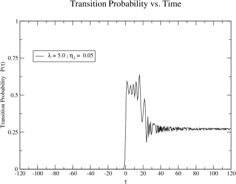
Figure 7: The transition probability $P(\tau)$ for non-adiabatic rapid passage with cubic twist with $\lambda=5.0$ and $\eta_{\,3}=0.05$.

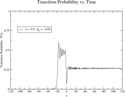
Figure 8: The transition probability $P(\tau)$ for non-adiabatic rapid passage with cubic twist with $\lambda=5.0$ and $\eta_{\,3}=-0.05$.

The avoided crossings in Figure 7 (8) clearly occur at $\tau=0$ and $\tau=20$ ($-20$) as expected. Here the avoided crossings interfere destructively, with $P=0.270$. Summarizing, we see that: (1) two avoided crossings do occur during rapid passage with cubic twist as predicted in Table 1; (2) the avoided crossings produce interference effects in the asymptotic transition probability $P$ which can be controlled through variation of their separation; and (3) the separation of the avoided crossings $\Delta\tau_{ac}=|\tau_{2}-\tau_{1}|=1/|\eta_{\,3}|$ can be altered by varying $\eta_{\,3}=\hbar Bb/a^{2}$. We now consider two possible applications of this interference effect.

III.2 Non-Resonant Pump

First, consider twistless adiabatic rapid passage with $\lambda=0.5$ and $\eta_{\,3}=0$. Figure 9 show the transition probability $P(\tau)$ for this case. The asymptotic transition probability is $P=1.87\times 10^{-3}$.

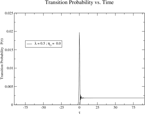
Figure 9: The transition probability $P(\tau)$ for twistless adiabatic rapid passage with $\lambda=0.5$ and $\eta_{\,3}=0$. Note the greatly reduced vertical scale compared to previous figures.

Figure 10 shows $P(\tau)$ for adiabatic rapid passage with cubic twist with $\lambda=0.5$ and $\eta_{\,3}=0.04$.

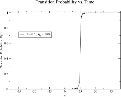
Figure 10: The transition probability $P(\tau)$ for adiabatic rapid passage with cubic twist with $\lambda=0.5$ and $\eta_{\,3}=0.04$.

The asymptotic transition probability in this case is $P=0.996$! Thus, by introducing a small amount of cubic twist, constructive interference between the avoided crossings transforms adiabatic rapid passage into a non-resonant pump for the qubit energy levels. Figures 5 and 6 indicate that, should it be desired, equally large transition probabilities are also possible at faster inversion rates $\lambda$. It is worth pointing out that to produce such a large transition probability using twistless non-adiabatic rapid passage would require $\lambda=784$ (see eqn. (23) with $\eta_{\,2}=0$) as opposed to $\lambda\sim 0.5-5.0$ when cubic twist is exploited.

III.3 Transition Quenching

We now show that one can utilize the interference between avoided crossings to strongly suppress qubit transitions during non-adiabatic rapid passage with cubic twist. Figure 11 shows $P(\tau)$ for $\lambda=5.0$ and $\eta_{\,3}=4.577\times 10^{-2}$.

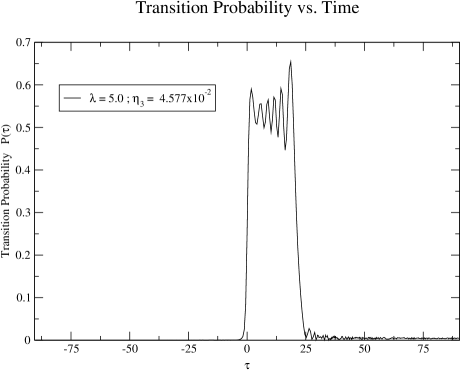
Figure 11: The transition probability $P(\tau)$ for non-adiabatic rapid passage with cubic twist with $\lambda=5.0$ and $\eta_{\,3}=4.577\times 10^{-2}$. Note the slightly reduced vertical scale.

The asymptotic transition probability for this case is $P=3.44\times 10^{-3}$. This is to be compared with twistless rapid passage with $\lambda=5.0$ (Figure 4) for which $P=0.533$. Destructive interference between the two avoided crossings has reduced the transition probability $P$ by 2 orders of magnitude relative to the twistless case shown in Figure 4. Thus if we were to implement a fast NOT-operation using non-adiabatic rapid passage with cubic twist at $\lambda=5.0$ and $\eta_{\,3}=4.577\times 10^{-2}$, we would obtain (on average) 1 bit-flip error per 291 NOT-operations. By comparison, twistless rapid passage with $\lambda=5.0$ would produce (on average) 1 bit-flip error for every 2 NOT-operations. This result strongly suggest the value of exploring whether this destructive interference between avoided crossings during twisted rapid passage could be exploited to produce fast reliable quantum NOT and CNOT logic gates. As striking as this result for cubic twist is, we shall see in the following Section that quartic twist can reduce the bit-flip error probability even more dramatically.

IV Quartic Twist

For quartic twist $\phi_{4}(t)=(1/2)Bt^{4}$ and $\eta_{\,4}=\hbar Bb^{2}/a^{3}$. Avoided crossings are expected to occur at $\tau_{1}=0$, and at $\tau_{2}=\pm 1/\sqrt{\eta_{\,4}}$ (when $sgn\,\eta_{\,4}=+1$; see eqn. (20) and Table 1). Formally, the analysis of quartic twist parallels that of quadratic and cubic twist. With the substitution $\phi_{2}(t)\rightarrow\phi_{4}(t)$, eqns. (21) and (22) continue to apply, and one determines $\overline{\Gamma}(\tau)$ and $\overline{\delta}(\tau)$ from eqns. (22b) and (22c). Once $\overline{\Gamma}(\tau)$ and $\overline{\delta}(\tau)$ are known, eqns. (15) can be integrated numerically subject to the initial condition specified in eqns. (16).

IV.1 Demonstration of Quantum Interference

In Figure 12 we plot the transition probability $P(\tau)$ for $\lambda=5.0$ and $\eta_{\,4}=4.6\times 10^{-4}$.

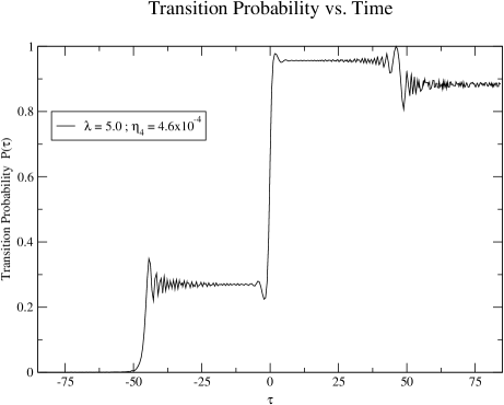
Figure 12: The transition probability $P(\tau)$ for non-adiabatic rapid passage with quartic twist with $\lambda=5.0$ and $\eta_{\,4}=4.6\times 10^{-4}$.

The expected avoided crossings at $\tau_{1}=0$ and $\tau_{2}=\pm 46.63$ are clearly visible. The asymptotic transition probability for this case is $P=0.88$. For twistless rapid passage with $\lambda=5.0$ (see Figure 4), $P=0.533$. Thus the avoided crossings in Figure 12 are constructively interfering, leading to an enhancement of the transition probability $P$. Figure 13 shows $P(\tau)$ for quartic twist with $\lambda=5.0$ and $\eta_{\,4}=-4.6\times 10^{-4}$.

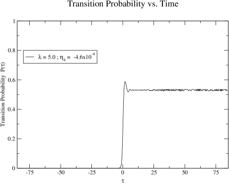
Figure 13: The transition probability $P(\tau)$ for non-adiabatic rapid passage with quartic twist with $\lambda=5.0$ and $\eta_{\,4}=-4.6\times 10^{-4}$.

This Figure clearly shows only one avoided crossing at $\tau_{1}=0$, as expected for $sgn\,\eta_{\,4}=-1$ (see Table 1). The asymptotic transition probability in this case is $P=0.533$ which equals the result for twistless rapid passage with $\lambda=5.0$ (Figure 4) to the level of precision obtained in our calculation.

Figure 14 plots $P(\tau)$ for $\lambda=5.0$ and $\eta_{\,4}=1.6\times 10^{-3}$.

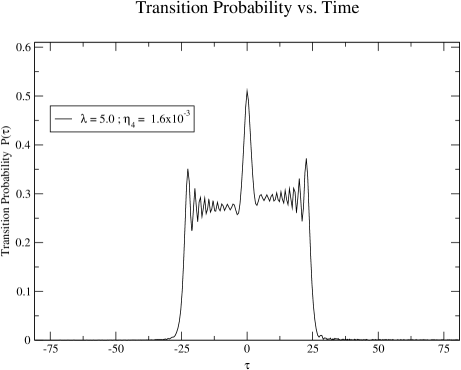
Figure 14: The transition probability $P(\tau)$ for non-adiabatic rapid passage with quartic twist with $\lambda=5.0$ and $\eta_{\,4}=1.6\times 10^{-3}$. Note the slightly reduced vertical scale.

The Figure clearly shows the expected crossings at $\tau_{1}=0$ and $\tau_{2}=\pm 25.0$. The asymptotic transition probability is $P=6.93\times 10^{-4}$ and corresponds to destructive interference relative to twistless rapid passage with $\lambda=5.0$ (Figure 4). We do not include a plot of $P(\tau)$ for $\lambda=5.0$ and $\eta_{\,4}=-1.6\times 10^{-3}$ as it is similar to Figure 13: one avoided crossing at $\tau_{1}=0$ and $P=0.533$.

Summarizing these results, we see that: (i) three (one) avoided crossings (crossing) occur(s) as predicted in Table 1 when $sgn\,\eta_{\,4}=+1\;(-1)$; (ii) the avoided crossings produce interference effects in the transition probability, with the character of the interference (constructive or destructive) determined by the separation of the avoided crossings; and (iii) the separation of adjacent avoided crossings is given by $\Delta\tau_{ac}=|\tau_{2}-\tau_{1}|=1/\sqrt{\eta_{\,4}}$ ($sgn\,\eta_{\,4}=+1$), and it is controllable through variation of $\eta_{\,4}=\hbar Bb^{2}/a^{3}$.

IV.2 Non-Resonant Pump

Quartic twist does not appear to be as effective at pumping the qubit energy-levels as cubic twist. Figure 15 shows $P(\tau)$ for $\lambda=0.5$ and $\eta_{\,4}=6.45\times 10^{-3}$.

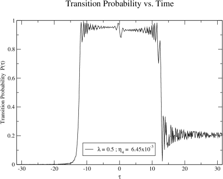
Figure 15: The transition probability $P(\tau)$ for adiabatic rapid passage with quartic twist with $\lambda=0.5$ and $\eta_{\,4}=6.45\times 10^{-3}$.

The expected avoided crossings at $\tau_{1}=0$ and $\tau_{2}=\pm 12.45$ are clearly visible, and the asymptotic transition probability is $P=0.20$. Although this is a 2 order of magnitude improvement over twistless adiabatic rapid passage with $\lambda=0.5$ (Figure 9), it falls well short of the transition probability $P=0.996$ easily obtainable with cubic twist. In fact, for $\eta_{\,4}<1$, $P\sim 0.20$ was among the largest $P$-values we could find. If larger values of twist strength are allowed, the largest transition probability we could find was $P=0.64$ at $\eta_{\,4}=3.00$.

IV.3 Transition Quenching

Quartic twist proves to be much more effective at quenching transitions during non-adiabatic rapid passage than cubic twist. Table 2 gives the transition probabilities for quartic twist pulses for which $\lambda=5.00$ and $\eta_{4}$ lies in the interval [$3.95\times 10^{-3}$, $4.04\times 10^{-3}$].

Table 2: Transition probabilities for quartic twist with $\lambda=5.00$ and $\eta_{4}$ in the range [$3.95\times 10^{-3}$, $4.04\times 10^{-3}$].

$\>\eta_{4}\;\;(\,\times 10^{-3}\,)\;$	$P$
3.95	$2.0\times 10^{-2}$
3.96	$1.3\times 10^{-2}$
3.97	$6.8\times 10^{-3}$
3.98	$3.6\times 10^{-3}$
3.99	$9\times 10^{-4}$
4.00	$4\times 10^{-5}$
4.01	$8\times 10^{-4}$
4.02	$3.9\times 10^{-3}$
4.03	$1.0\times 10^{-2}$
4.04	$1.7\times 10^{-2}$

The essential thing to notice in Table 2 is that for $\eta_{4}=4.00\times 10^{-3}$, the transition probability $P=4\times 10^{-5}$. This is significant for the following reason. It has been shown that a quantum computation of arbitrarily long duration becomes possible if the quantum logic gates used to implement the computation all have error probabilities (per gate operation) which lie below the threshold $P_{ft}$ for fault tolerant operation pre . This threshold has been estimated to be $P_{ft}\sim 10^{-4}-10^{-5}$ flt . In terms of the gate fidelity $F=1-P$, the more optimistic estimate for $P_{ft}$ gives $F_{ft}=0.9999$. We see that for $\lambda=5.00$ and $\eta_{4}=4.00\times 10^{-3}$, twisted rapid passage with quartic twist gives a gate fidelity of $F=0.99996$ which exceeds the best case estimate for fault tolerant operation $F_{ft}=0.9999$. This fault tolerant performance is achieved while inverting the qubit at a non-adiabatic rate. The reader should note that the values $\lambda=5.00$ and $\eta_{4}=4.0\times 10^{-3}$ can be realized with existing NMR technology (see Section V.4). Our analysis raises the exciting possibility that non-adiabatic rapid passage with quartic twist might provide a means of realizing fast fault-tolerant NOT and CNOT gates. The novelty of this prospect is the marriage of operational speed with fault-tolerance. This marriage of speed and reliability is a direct consequence of the destructive interference which is possible between the 3 avoided crossings that arise during rapid passage with quartic twist. Quantum CNOT gates are ubiquitous in quantum computing and quantum error correction uni ; bar ; qec . Thus, determining how to implement them in a fast fault tolerant manner is a potentially significant development for the field.

V Discussion

V.1 Summary

It has been our aim in this paper to show that multiple avoided crossings can arise during twisted rapid passage, and that by varying their time-separation, interference effects are produced which allow for a direct control over qubit transitions. This time-separation is controlled through the (dimensionless) twist strength $\eta$, and the resulting interference can be constructive (enhancing transitions) or destructive (reducing transitions). For nth-order polynomial twist, $\eta_{\,n}=\hbar Bb^{n-2}/a^{n-1}$, where $B$ is the (dimensionful) twist strength, $2b$ is the energy-gap separating the qubit energy-levels at an avoided crossing, and $a$ is the inversion rate of the external field $\mathbf{F}(t)$ (see Section II). The interference effects are a consequence of the temporal phase coherence of the wavefunction. The ability to vary this coherence by varying the temporal separation of the avoided crossings renders twisted rapid passge with adjustable twist strength into a temporal interferometer through which qubit transitions can be greatly enhanced or suppressed. Cubic and quartic twist were explicitly considered in this paper as they are, respectively, the simplest examples of odd-order and even-order polynomial twist in which these interference effects are expected to occur. Although we have focused on these two cases, we do not mean to suggest that these pulses are the best of all possible twisted rapid passage pulses. A search is currently underway for other twisted rapid passage pulses that might produce stronger destructive interference, and hence, faster, more fault tolerant quantum CNOT and NOT gates (see below for further discussion). We have seen that this interference mechanism can be used to pump qubit energy-levels, as well as to strongly quench qubit transitions during non-adiabatic twisted rapid passage. Although cubic twist proved to be more effective at pumping than quartic twist, quartic twist was found to be much more effective at quenching qubit transitions. We have seen that quartic twist allows qubit inversion to be done both non-adiabatically and at fidelities that exceed the threshold for fault tolerant operation. The marriage of operational speed with reliability is a direct consequence of the destructive interference that is possible between the 3 avoided crossings that can arise during rapid passage with quartic twist.

V.2 Implementing Quantum CNOT Gate

We now describe a procedure for implementing a quantum CNOT gate using twisted rapid passage in the context of liquid state NMR. If the liquid has low viscosity, one can ignore dipolar coupling between the qubits, and if the remaining Heisenberg interaction between the qubits is weak compared to the individual qubit Zeeman energies, it can be well-approximated by an Ising interaction chu . Under these conditions, the Hamiltonian (in frequency units) for the control ($c$) and target ($t$) qubits is:

$$\frac{H_{ct}}{\hbar}=-\omega_{c}\,I^{c}_{z}-\omega_{t}\,I^{t}_{z}+2\pi J\,I^{c}_{z}\,I^{t}_{z}\hskip 7.22743pt.$$ (24)

Here $\omega_{c}$ ($\omega_{t}$) is the resonance frequency of the isolated control (target) qubit; $J$ is the Ising coupling constant; and $\omega_{c}>\omega_{t}>\pi J$. We choose the single qubit computational basis states (CBS) to be $|0\rangle=|\uparrow\rangle$ and $|1\rangle=|\downarrow\rangle$. Thus the two-qubit CBS are: $|00\rangle=|\uparrow\uparrow\rangle$; $|01\rangle=|\uparrow\downarrow\rangle$; $|10\rangle=|\downarrow\uparrow\rangle$; and $|11\rangle=|\downarrow\downarrow\rangle$, and they are the eigenstates of $H_{ct}$. The energy-levels (in frequency units) are shown in Figure 16, where

$$\omega_{\pm}=\omega_{t}\pm\pi J\hskip 7.22743pt.$$ (25)

Figure 16: Energy-level structure appropriate for implementing a quantum CNOT operation using twisted rapid passage. The corresponding energies (in frequency units) appear to the right of the energy levels.

Given this energy-level structure, we can implement a quantum CNOT operation on the two qubits by sweeping through the $\omega_{+}$ resonance using twisted rapid passage. Decoupling ch2 is used to switch off the dynamics of the control qubit so that only the target qubit responds to the rapid passage pulse. Since the two states $|00\rangle$ and $|01\rangle$ are not resonant, they do not respond to the twisted rapid passage pulse. Thus,

$$\begin{array}[]{l}|00\rangle\rightarrow|00\rangle\\ |01\rangle\rightarrow|01\rangle\hskip 7.22743pt.\end{array}$$ (26)

On the other hand, for the $|10\rangle$ and $|11\rangle$ states, the combination of decoupling and sweeping through the $\omega_{+}$ resonance means that only the target qubit has its spin flipped. Thus,

$$\begin{array}[]{l}|10\rangle\rightarrow|11\rangle\\ |11\rangle\rightarrow|10\rangle\hskip 7.22743pt,\end{array}$$ (27)

and we see that this procedure implements a quantum CNOT operation on the two qubits.

V.3 Experimental Realization

Because of the fundamental significance of quantum CNOT gates to quantum computing and quantum error correction uni ; bar ; qec , it is hoped that the feasibility of using rapid passage with quartic twist to implement this gate might be tested experimentally (see penultimate paragraph of Section I). Experimental realization of polynomial twist $\phi_{n}(t)=(2/n)Bt^{n}$ should be possible through an adaptation of the procedure used by Zwanziger et. al. zwa to realize quadratic twist. Thus: (1) the driving rf-field is linearly polarized along the x-axis in the lab-frame with $F_{x}(t)=2b\cos\phi_{rf}(t)$; (2) the resonance offset $at$ (see eqn. (1)) is produced by linearly sweeping the detector frequency $\omega_{det}(t)$ through the resonance at the Larmor frequency $\omega_{0}$ such that $\omega_{det}(t)=\omega_{0}+(2at/\hbar)$; and (3) twist is introduced by sweeping the rf-frequency $\omega_{rf}(t)=\dot{\phi}_{rf}$ through the resonance at $\omega_{0}$ in such a way that $\omega_{rf}(t)=\omega_{det}-\dot{\phi}_{n}$. It is worth noting that the resonance condition $\omega_{rf}(t)=\omega_{0}$ is identical to our existence condition for avoided crossings, eqn. (5). Note that in our paper the external field inversion takes place over the time-interval ($-T_{0}/2$, $T_{0}/2$); the external field crosses the x-y plane at $t=0$ and is initially aligned along the $-\hat{\mathbf{z}}$ direction. The Appendix provides a translation key which relates the theoretical parameters of this paper to the experimental parameters of the Zwanziger experiments jwz ; zwa .

Before leaving the subject of experimental realization of rapid passage with quartic twist, two further remarks are in order. First, to insure that all qubits are inverted when a spread of resonance frequencies occurs, it is necessary to require that the frequency sweep cover a large enough interval that the entire spread of resonance frequencies is included in it. This gaurantees that all qubits will have passed through resonance by the end of the frequency sweep. Second, a range of rf field strengths can also be accomodated so long as $aT/2\gg b_{max}$. This condition insures that the frequency sweep begins far from resonance for all rf field strengths, and that transitions will continue to occur only near the avoided crossings. One therefore anticipates that in this case also, the interference effects will continue to occur as predicted. For reasonably good samples, magnets, and rf sources these constraints can be satisfied, and the interference effects presented above should be readily observable. This is in fact what is found experimentally jwz .

V.4 Other Pulses

Having introduced twisted rapid passage with polynomial twist, and pointed out the possible advantages of quartic twist for quantum computing, it is natural to ask how quartic twist compares with the more familiar $\pi$-pulse which can also be used to implement quantum CNOT and NOT gates. We begin by comparing the inversion time for quartic twist with that of a comparable $\pi$-pulse. We focus on quartic twist with $\lambda=5.00$ and $\eta_{4}=4.00\times 10^{-3}$ as this choice of parameters yields a gate fidelity $F=0.99996$ (see Section IV.3) which exceeds the threshold for fault tolerant gate operation $F_{ft}\sim 0.9999$. We now show that this case achieves fault tolerant operation while simultaneously matching the inversion speed of a $\pi$-pulse. In the notation of Ref. zwa , the basic experimental parameters for twisted rapid passage are $A$, $B$, $\omega_{1}$, and $T$, and they are related to our theoretical parameters by eqns. (35) and (30). $T$ continues to denote the duration of the twisted rapid passage pulse. Because a twisted rapid passage sweep must begin far from the avoided crossings, $A$ and $\omega_{1}$ cannot be chosen independently. In the rf-frame, the asymptotic effective magnetic field must lie near the z-axis so that $\tan\theta=\omega_{1}/A\sim 0.1$. Choosing $\omega_{1}=4000$ Hz gives $A=4\times 10^{4}$ Hz. Both of these values can be achieved with existing NMR technology. Writing $f=\omega_{1}/A$, eqn. (36) gives

$$T_{4}=\frac{4}{f\omega_{1}\lambda}\hskip 7.22743pt.$$

With $\lambda=5.00$, this gives

$$T_{4}=2\;\textrm{msec}\hskip 7.22743pt.$$

By comparison, the inversion time for a $\pi$-pulse with rf-amplitude $\omega_{1}=4000$ Hz is $T_{\pi}=\pi/\omega_{1}=0.8$ msec. Thus, twisted rapid passage with quartic twist is clearly capable of matching the inversion speed of a comparable $\pi$-pulse while still exceeding the threshold for fault tolerant operation. On the other hand, the error probability for a typical $\pi$-pulse is $P\sim 10^{-3}$ due to, for example, inhomogenities in the rf field amplitude. This corresponds to a fidelity $F\sim 0.999$ so that, unlike the equally fast quartic twist pulse which acts fault tolerantly, the $\pi$-pulse falls short of the threshold for fault tolerant operation $F_{th}\sim 0.9999$.

We hope in the future to examine higher order versions of polynomial twist to determine whether they have more effective quenching and/or robustness properties than cubic and quartic twist. We have also done preliminary work on the interesting case of periodic twist: $\phi(t)=\pi\rho\sin\omega t$. As we have seen, polynomial twist only allows 1–3 avoided crossings to occur during rapid passage. One can show that periodic twist allows the number of avoided crossings that occur during rapid passage to be modified through variation of the twist amplitude $\rho$ and frequency $\omega$. We intend to explore how the interference effects considered here are modified when more than 3 avoided crossings can occur.

Appendix A Connection Between Theory and Experiment

For ease of comparison with Refs. zwa and jwz , we choose $\mathbf{F}(t)=-b\cos\phi_{n}(t)\hat{\mathbf{x}}-b\sin\phi_{n}(t)\hat{\mathbf{y}}+at\hat{\mathbf{z}}$ in eqn. (1). The Hamiltonian in the detector frame is then

$$\frac{H(t)}{\hbar}=\frac{at}{\hbar}\,\sigma_{z}-\frac{b}{\hbar}\,\cos\phi_{n}(t)\,\sigma_{x}-\frac{b}{\hbar}\,\sin\phi_{n}(t)\,\sigma_{y}\hskip 7.22743pt.$$

Here $\phi_{n}(t)=(2/n)\mathcal{B}t^{n}$, and to avoid confusion with the notation of Ref. zwa , we have switched the symbol used for the twist strength in the main body of this paper: $B\rightarrow\mathcal{B}$. Transformation to the rf-frame is done using the unitary operator $U(t)=\exp[-(i/2)\,\phi_{n}(t)\,\sigma_{z}]$ so that $H(t)\rightarrow\overline{H}(t)$:

$$\frac{\overline{H}(t)}{\hbar} = \left(\,\frac{at}{\hbar}-\frac{\dot{\phi}_{n}}{2}\,\right)\,\sigma_{z}-\frac{b}{\hbar}\,\sigma_{x}$$ (28)

$$= \left(\,\frac{2at}{\hbar}-\dot{\phi}_{n}\,\right)\,I_{z}-\frac{2b}{\hbar}\,I_{x}\hskip 7.22743pt,$$

and $\mathbf{I}=\mathbf{\sigma}/2$.

The experimental Hamiltonian in the rf-frame appears in eqn. (12) of Ref. zwa :

$$\frac{\overline{H}_{ex}(t)}{\hbar}=\left(\,\dot{\phi}_{rf}-\omega_{0}\,\right)\,I_{z}-\omega_{1}\,I_{x}\hskip 7.22743pt.$$ (29)

Comparing eqns. (28) and (29) gives

$$\omega_{1}=\frac{2b}{\hbar}$$ (30)

and

$$\dot{\phi}_{rf}-\omega_{0}=\frac{2at}{\hbar}-\dot{\phi}_{n}\hskip 7.22743pt.$$ (31)

Integrating eqn. (31) gives

$$\phi_{rf}(t^{\prime\prime})=\int_{-T/2}^{t^{\prime\prime}}\,dt^{\prime\prime\prime}\,\left[\,\omega_{0}+\frac{2aT}{\hbar}\left(\,\frac{t^{\prime\prime\prime}}{T}\,\right)-2\mathcal{B}T^{n-1}\,\left(\,\frac{t^{\prime\prime\prime}}{T}\,\right)^{n-1}\,\right]\hskip 7.22743pt.$$ (32)

In this paper, we have parameterized time such that $t^{\prime\prime\prime}\in[\,-T/2,T/2\,]$, and $T$ is the duration of the twisted rapid passage pulse. Defining

$$\tau=\frac{t^{\prime\prime\prime}}{T}+\frac{1}{2}\hskip 7.22743pt,$$

it follows that $\tau\in[0,1]$. Introducing $t^{\prime}=t^{\prime\prime\prime}+T/2$ and $t=t^{\prime\prime}+T/2$, eqn. (32) becomes

$$\phi_{rf}(t)=\int_{0}^{t}\,dt^{\prime}\,\left[\,\omega_{0}+\left(\,\frac{2aT}{\hbar}\,\right)\,\left(\,\tau-\frac{1}{2}\,\right)-\frac{2\mathcal{B}T^{n}}{T}\,\left(\,\tau-\frac{1}{2}\,\right)^{n-1}\,\right]\hskip 7.22743pt.$$ (33)

As explained in the caption of Figure 2 of Ref. zwa , $\dot{\phi}_{rf}=\dot{\phi}_{det}-\dot{\phi}_{n}$; with $\dot{\phi}_{det}=\omega_{0}+2A(\tau-1/2)$; and generalizing to polynomial twist, $\dot{\phi}_{n}=nB(\tau-1/2)^{n-1}/T$, where $B$ is the symbol used in Ref. zwa for the twist strength. Plugging these expressions for $\dot{\phi}_{det}$ and $\dot{\phi}_{n}$ into $\dot{\phi}_{rf}=\dot{\phi}_{det}-\dot{\phi}_{n}$, and integrating gives

$$\phi_{rf}(t)=\int_{0}^{t}\,dt^{\prime}\,\left[\,\omega_{0}+2A\left(\,\tau-\frac{1}{2}\,\right)-\frac{nB}{T}\,\left(\,\tau-\frac{1}{2}\,\right)^{n-1}\,\right]\hskip 7.22743pt.$$ (34)

Equating eqns. (33) and (34) gives

$$A = \frac{aT}{\hbar}$$ (35a)

$$B = \frac{2\mathcal{B}}{n}T^{n}\hskip 7.22743pt.$$ (35b)

Using eqns. (30) and (35) in the definition of $\lambda$ (see discussion following eqns. (22)) gives

$$\lambda=\frac{4\,|A|}{\omega_{1}^{2}T}\hskip 7.22743pt.$$ (36)

Using eqns. (30), (35) and eqn. (18) with $n=3$ and $4$ gives

$$\eta_{3}=\frac{3}{4}\,\frac{B\omega_{1}}{A^{2}T}$$ (37)

and

$$\eta_{4}=\frac{B\omega_{1}^{2}}{2A^{3}T}\hskip 7.22743pt,$$ (38)

respectively. The results of this Appendix give the connection between our theoretical parameters and the experimental parameters $A$, $B$, $\omega_{1}$, and $T$ of the Zwanziger experiments jwz ; zwa . In Section V, these formulas are used to calculate the inversion time for a twisted rapid passage pulse with quartic twist.

References

- (1) A. Abragam, Principles of Nuclear Magnetism (Oxford University Press, New York 1961).
- (2) M. V. Berry, Proc. R. Soc. Lond. A 430, 405 (1990).
- (3) J. W. Zwanziger, S. P. Rucker, and G. C. Chingas, Phys. Rev. A 43, 3232 (1991).
- (4) J. W. Zwanziger, U. Werner-Zwanziger, and F. Gaitan, submitted to Chem. Phys. Lett. .
- (5) R. Lim, J. Phys. A 26, 7615 (1993).
- (6) K-A Suominen and B. M. Garraway, Phys. Rev. A 45, 374 (1992); K-A Suominen, Opt. Commun. 93, 126 (1992); K-A Suominen, B. M. Garraway, and S. Stenholm, Opt. Commun. 82, 260 (1991).
- (7) A. Joye, J. Phys. A 26, 6517 (1993); A. Joye, G. Mileti, and C. E. Pfister, Phys. Rev. A 44, 4280 (1991).
- (8) L. Landau, Phys. Z. Sowjetunion 1, 46 (1932)
- (9) C. Zener, Proc. R. Soc. Lond. A 137, 696 (1932).
- (10) A. Shapere and F. Wilczek, Geometric Phases in Physics (World Scientific, New Jersey, 1989).
- (11) W. R. Thorson, J. B. Delos, and S. A. Boorstein, Phys. Rev. A 4, 1052 (1971).
- (12) J. Preskill, Proc. R. Soc. Lond. A 454, 385 (1998).
- (13) P. Shor, in Proceedings of the 37th Symposium on the Foundations of Computer Science, (IEEE Computer Society Press, Los Alamitos, CA 1996), pp. 56-65; D. Gottesman, PhD thesis preprint http://www.arxiv.org/quant-ph/9705052.
- (14) D. P. DiVincenzo, Proc. R. Soc. Lond. A 454, 261 (1998).
- (15) A. Barenco et. al. , Phys. Rev. A 52, 3457 (1995).
- (16) P. W. Shor, Phys. Rev. A 52, R2493 (1995); A. M. Steane, Proc. R. Soc. Lond. A 452, 2551 (1996); A. R. Calderbank and P. W. Shor, Phys. Rev. A 54, 1098 (1996); D. Gottesman, Phys. Rev. A 54, 1862 (1996); E. Knill and R. Laflamme, Phys. Rev. A 55, 900 (1997); see also A. M. Steane, in Introduction to Quantum Computation and Information, eds. H. K. Lo, S. Popescu, and T. Spiller (World Scientific, New Jersey, 1998).
- (17) N. A. Gershenfeld and I. L. Chuang, Science 275, 350 (1997).
- (18) I. L. Chuang, in Introduction to Quantum Computation and Information, eds. H. K. Lo, S. Popescu, and T. Spiller (World Scientific, New Jersey, 1998).