Persistent currents due to point obstacles

a) Laboratory of Physics, Kochi University of Technology,
e)xTosa Yamada, Kochi 782-8502, Japan
b) Department of Theoretical Physics, Nuclear Physics Institute,
e)xAcademy of Sciences, 25068 Řež, Czech Republic
c) Doppler Institute, Czech Technical University, Břehová 7,
e)x11519 Prague, Czech Republic
e)xtaksu.cheon@kochi-tech.ac.jp, exner@ujf.cas.cz

We discuss properties of the two-dimensional Landau Hamiltonian perturbed by a family of identical $\delta$ potentials arranged equidistantly along a closed loop. It is demonstrated that for the loop size exceeding the effective size of the point obstacles and the cyclotronic radius such a system exhibits persistent currents at the bottom of the spectrum. We also show that the effect is sensitive to a small disorder.

1 Introduction

Persistent currents in rings threaded by a magnetic flux are one of the characteristic features of mesoscopic systems – see, e.g., [CGR, CWB] and numerous other theoretical and experimental papers where they were discussed. Recall that for a charged particle (an electron) confined to a loop $C$ the effect is contained in the dependence of the corresponding eigenvalues $E_{j}$ on the flux $\phi$ threading the loop measured in the units of flux quanta, $2\pi\hbar c|e|^{-1}$. Specifically the derivative $\partial E_{j}/\partial\phi$ equals $-{1\over c}I_{j}$, where $I_{j}$ is the persistent current in the $j$–th state. In particular, if the particle motion on the loop is free, we have

$$E_{j}(\phi)={\hbar^{2}\over 2m^{*}}\left(2\pi\over L\right)^{2}(j+\phi)^{2},$$ (1.1)

where $L$ is the loop circumference, so the currents depend linearly on the applied field.

The above example represents an ideal case when the particle is strictly confined to the loop. On the other hand, there are many situations when a particle in a magnetic field can be transported being localized essentially in the vicinity of a barrier or an interface. A prominent example are the edge currents [Ha, MS]. They attracted a new wave of interest recently when in several papers [BP, FGW, FM, MMP] conditions were derived under which such a transport remained preserved in the presence of a disorder.

Even weaker interaction giving rise to a magnetic transport, this time without a classical analogue, was found in [EJK], where the Landau Hamiltonian was perturbed by a straight equidistant array of $\delta$ potentials. It was shown that such an operator has bands of absolutely continuous spectrum in the gaps between the Landau levels. An independent evidence for the transport in this situation was found in [Ue].

The question we are going to ask in this paper is the following. If we take a finite array of identical $\delta$ potentials in the plane making a loop, does the mentioned transport give rise to persistent currents? As we will see the answer is in general positive if the effective radii of the $\delta$ potentials (specified below – see (2.4)) and the cyclotronic radius corresponding to the field intensity are much smaller than the loop size. We also discuss the effect of disorder manifested by randomization of the coupling constants and show that the effect is sensitive to such perturbations: in an example with a ring of 12 obstacles a variation larger than 1% leads to a localization.

2 The model

2.1 2D magnetic systems with point obstacles

As we said above, we are going to study a charged particle in the plane subject to a homogeneous magnetic field perpendicular to the plane interacting with an equidistant array of point obstacles placed at points $\vec{a}_{j},\>j=1,\dots,N$, belonging to a closed loop. The simplest example is the situation when the latter is a circle,

$$\vec{a}_{j}=\left(R\,\cos{2\pi j\over N},\,R\,\sin{2\pi j\over N}\right)\,,\;j=1,\dots,N\,.$$ (2.1)

For the sake of brevity we shall write $\vec{a}:=(\vec{a}_{1},\dots,\vec{a}_{N})$. The obstacles will be modeled by $\delta$ potentials so formally the Hamiltonian of the system can be written as

$$H=\left(-i\vec{\nabla}-\vec{A}(\vec{x})\right)^{2}+\sum_{j=1}^{N}\tilde{\alpha}_{j}\delta(\vec{x}\!-\!\vec{a}_{j})\,,$$ (2.2)

where $\vec{A}$ is the appropriate vector potential which we choose here in the circular gauge,

$$\vec{A}(\vec{x})=\left(-{1\over 2}By,\,{1\over 2}Bx\right)\,.$$

To make things simple we have used rationalized units in (2.2) putting $\hbar=c=e=2m^{*}=1$. On the other hand, the two-dimensional $\delta$ interaction is an involved object. To give it meaning and to specify the true coupling parameter which would replace the formal $\tilde{\alpha}_{j}$’s, we use the definition based on self-adjoint extensions which is discussed thoroughly in [AGHH], see also [DO, GHŠ] for the situation with a magnetic field. A $\delta$ interaction is determined by means of the boundary conditions

$$L_{1}(\psi,\vec{a}_{j})+2\pi\alpha_{j}L_{0}(\psi,\vec{a}_{j})=0\,,\quad j=1,\dots,N\,,$$ (2.3)

which couple the generalized boundary values

$$L_{0}(\psi,\vec{a}):=\lim_{|\vec{x}-\vec{a}|\to 0}\,{\psi(\vec{x})\over\ln|\vec{x}\!-\!\vec{a}|}\,,\;L_{1}(\psi,\vec{a}):=\lim_{|\vec{x}-\vec{a}|\to 0}\Bigl{[}\psi(\vec{x})\!-\!L_{0}(\psi,\vec{a})\,\ln|\vec{x}\!-\!\vec{a}|\Bigr{]}\,.$$

We now put $\alpha:=(\alpha_{1},\dots,\alpha_{N})$ and denote by $H^{B}_{\alpha,\vec{a}}$ the Hamiltonian of our model, which acts as free outside the interaction support,

$$H^{B}_{\alpha,\vec{a}}\psi(\vec{x})=\left(-i\vec{\nabla}-\vec{A}(\vec{x})\right)^{2}\psi(\vec{x})$$

for $\vec{x}\not\in\vec{a}$, and its domain consists of all functions which belong to the Sobolev class $W^{2,2}(\mathbb{R}^{2}\setminus\vec{a})$ and satisfy the boundary conditions (2.3).

The parameters $\alpha_{j}$ characterizing the “strength” of the interaction are not trivial [EŠ, CS]; this is clear from the fact that the free (Landau) Hamiltonian, which we denote as $H^{B}$, corresponds to $\alpha_{j}=\infty,\>j=1,\dots,N$. The difference between $\alpha_{j}$ and the formal coupling constants used in (2.2) reflects the nontrivial way in which the two-dimensional point interaction arises in the limit of scaled potentials. To understand the $\alpha_{j}$’s it is more natural to associate them with the scattering length: by [EŠ] the point interaction with the parameter $\alpha$ reproduces the low-energy behaviour of the scattering upon an obstacle of the radius $\rho$ provided

$$\alpha={1\over 2\pi}\,\ln\rho\,.$$ (2.4)

2.2 Spectral properties of $H^{B}_{\alpha,\vec{a}}$

The spectrum of the free operator $H^{B}$ is the series of infinitely degenerate eigenvalues $B(2n+1),\>n=0,1,\dots\,$. A finite number of point interactions leaves the essential spectrum intact so $\sigma_{\mathrm{ess}}(H^{B}_{\alpha,\vec{a}})$ consists again of the Landau levels. Moreover, it follows from general principles [We, Sec .8.3] that $N$ point interactions can give rise to at most $N$ eigenvalues in each gap of $\sigma(H^{B})$. It is this discrete spectrum which is the object of our interest.

To find it we can make use of Krein’s formula [AGHH, App. A] which expresses the resolvent kernel of $H^{B}_{\alpha,\vec{a}}$ by means of that of the free operator, specifically

$$(H^{B}_{\alpha,\vec{a}}-\!z)^{-1}(\vec{x},\vec{x}^{\prime})=G_{B}(\vec{x},\vec{x}^{\prime};z)+\sum_{j,m=1}^{N}[\Lambda^{B}_{\alpha,\vec{a}}(z)]^{-1}_{jm}G_{B}(\vec{x},\vec{a}_{j};z)G_{B}(\vec{a}_{m},\vec{x}^{\prime};z),$$ (2.5)

where $\Lambda^{B}\equiv\Lambda^{B}_{\alpha,\vec{a}}(z)$ is the $N\times N$ matrix with the elements

$$\Lambda^{B}_{jm}:=\left(\alpha_{j}-\xi(B;z)\right)\delta_{jm}-G_{B}(\vec{a}_{j},\vec{a}_{m};z)(1\!-\!\delta_{jm})\,,$$

where $G_{B}(\vec{x},\vec{x}^{\prime};z)$ is the resolvent kernel of $H^{B}$ and $\xi(B;z)$ its regularized value at the singularity,

$$\xi(B;z):=\lim_{\vec{x}^{\prime}\to\vec{x}}\left[\,G_{B}(\vec{x},\vec{x}^{\prime};z)+{1\over 2\pi}\,\ln|\vec{x}-\vec{x}^{\prime}|\right]$$ (2.6)

which is independent of $\vec{x}$. The sought discrete spectrum is given by the singularities of the second term at the r.h.s. of (2.5), or in other words, by solutions of the spectral condition

$$\det\Lambda^{B}_{\alpha,\vec{a}}(z)=0\,.$$ (2.7)

If $z=z_{0}$ satisfies this, it is an eigenvalue of the operator $H^{B}_{\alpha,\vec{a}}$ and the equation $\Lambda^{B}_{\alpha,\vec{a}}(z_{0})d=0$ has a nontrivial solution in $\mathbb{C}^{N}$; the corresponding non-normalized eigenfunction is then

$$\psi^{B,z_{0}}_{\alpha,\vec{a}}=\sum_{j=1}^{N}d_{j}G_{B}(\vec{a}_{j},\cdot\,;z_{0})$$ (2.8)

as can be checked by a standard argument [AGHH].

To make use of the above formulae we need the explicit form of the free Green’s function. It is known [DMM] to be

$$G_{B}(\vec{x},\vec{x}^{\prime};z)={1\over 4\pi}\,\Phi_{B}(\vec{x},\vec{x}^{\prime})\,\Gamma\left(|B|\!-\!z\over 2|B|\right)\,U\left({|B|\!-\!z\over 2|B|},\,1;{|B|\over 2}|\vec{x}\!-\!\vec{x}^{\prime}|^{2}\right)\,,$$ (2.9)

where

$$\Phi_{B}(\vec{x},\vec{x}^{\prime}):=\exp\left[-{iB\over 2}(x_{1}\!-\!x^{\prime}_{1})(x_{2}\!+\!x^{\prime}_{2})-{|B|\over 4}|\vec{x}\!-\!\vec{x}^{\prime}|^{2}\right]$$

and $U(u,v;\zeta)$ is the singular confluent hypergeometric (or Kummer) function [AS, Chap. 13]. Using the asymptotic formula

$$U(u,1;\zeta)=-{1\over\Gamma(u)}\,\left[\,\ln\zeta+\psi(u)-2\psi(1)+\mathcal{(}O)(\zeta^{2}\ln^{2}\zeta)\,\right]$$

with $\psi(u)$ being the digamma function and $-\psi(1)=\gamma=0.577\dots$ the Euler number we find

$$\xi(B;z)=-{1\over 4\pi}\,\left[\,\psi\left(|B|\!-\!z\over 2|B|\right)+2\gamma+\ln{|B|\over 2}\,\right]\,.$$ (2.10)

In this way we have derived the explicit form of the matrix $\Lambda^{B}_{\alpha,\vec{a}}(z)$ appearing in the condition (2.7).

3 The results

In Fig. 1, we show the energy spectra of the system as a function of the common coupling strength $\alpha_{i}=\alpha$. In this example, the $Np=12$ of $\delta$-interactions are placed equidistantly on the ring of circumference $L=2\pi$. We can make this assumption without loss of generality. It is true that scaling systems with 2D point interactions reveals peculiar properties [CS2], but in effect changing the size of the system is equivalent to the shift of $\alpha$ on a constant proportional to logarithm of the scaling factor. One can see from this figure that, for our choice of the system size, the coupling becomes strong as the parameter approaches the value $\alpha=-1$, in which case the eigenvalues split from the Landau levels of unperturbed system form a bunch of negative-energy states; recall that by(2.4) it corresponds to the scattering length $\rho=e^{-2\pi}$.

The properties of these states are made clear by plotting their energies as the function of the magnetic field $B$. We set the strength parameter to be $\alpha=-1$. In the top lines of Fig. 2, several lowest states are shown for for three cases $Np=6$, $Np=12$ and $Np=24$. As the number of the $\delta$-scatterers increases, one clearly sees the emergence of parabolic $B$ dependence, which is the hallmark of the persistent current we have been looking for. The situation becomes clearer when we plot derivatives $dE/dB$ and $d^{2}E/dB^{2}$ as the function of $B$. A direct evidence of the existence of persistent current in our system is shown in Fig. 3, in which the probability flux current is depicted for $Np=12$ case for the magnetic field strengths $B=0.5$, $B=1.0$, $B=1.5$ and $B=2.0$.

As with the “usual” persistent currents, one has to take into account the imperfection when thinking about the use of the effect in designing various devices. Thus the question of the robustness of the persistent current in our system is of interest. We test it by allowing random fluctuation of the coupling strengths of the $\delta$-scatterers. In Fig. 4, we plot the $E$, $dE/dB$ and $d^{2}E/dB^{2}$ as the function of $B$ as before, but letting the coupling strength of each scatterer to vary randomly by the amount $\Delta\alpha$ uniformly around the central value $\alpha=-1$. The fluctuations are taken to be $\Delta\alpha=0.01$, $\Delta\alpha=0.02$ and $\Delta\alpha=0.03$ from the left to right. The number of $\delta$-scatterers is again set to be $Np=12$. Some examples of probability current flow patterns at $B=0.5$ for each case are shown in Fig. 5. While a more detailed analysis of such random perturbations is required, Figs. 4-5 suggest that the persistent current generated by the array of $\delta$-scatterers is sensitive to small fluctuations of the strength; one typically needs the accuracy of less the 1% to have the persistent current intact down to the ground state.

In conclusion, we have demonstrated a purely quantum mechanism able to create persistent currents in systems with arrays of tiny obstacles in magnetic field; it is the the wave nature of electrons which is responsible for this counterintuitive phenomenon. The result might eventually have a practical impact on the design of the quantum ring devices, however, the effect of localization by random perturbations deserves a deeper study.

Acknowledments

P.E. appreciates the hospitality extended to him at the Kochi University of Technology where a part of this work was done. The research has been partially supported by GAAS and the Czech Ministry of Education within the projects A1048101 and ME170, and also by Grant-in-Aid for Scientific Research (C) (No. 13640413) by the Japanese Ministry of Science and Education.

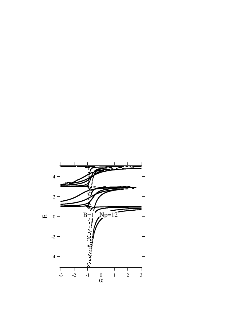
Figure 1: The energy spectra of a quantum particle on 2-dimensional plane with $Np=12$ delta functions of strength parameter $\alpha$ placed equidistantly on a ring of radius $R=1$ and subjected to perpendicular magnetic field of constant strength $B=1$. All quantities are in the unit $\hbar=c=e=2m*=1$.

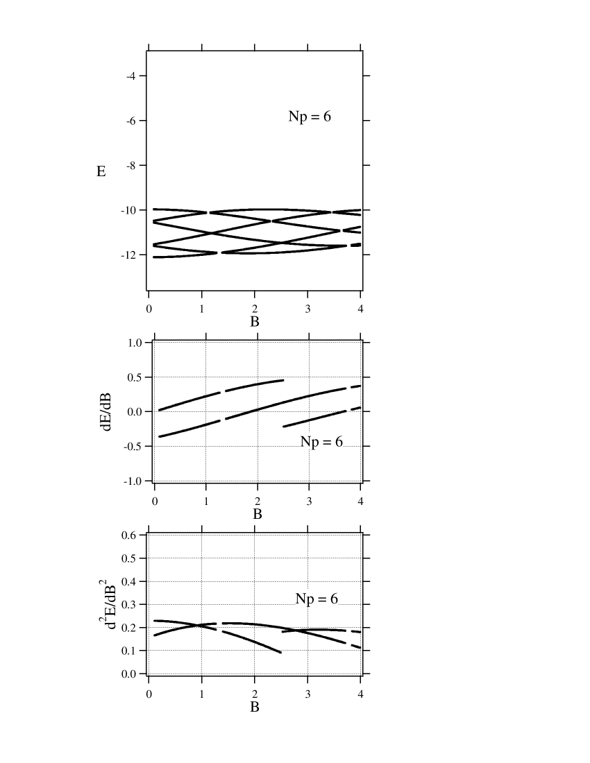
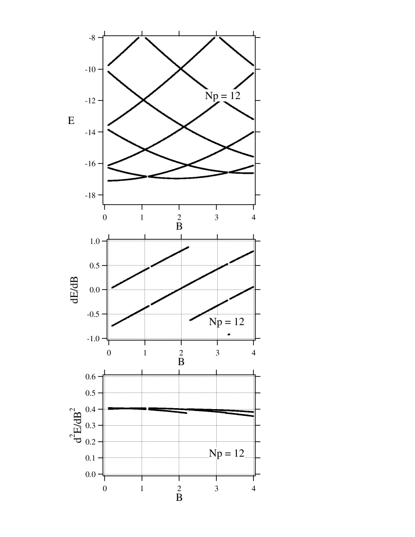
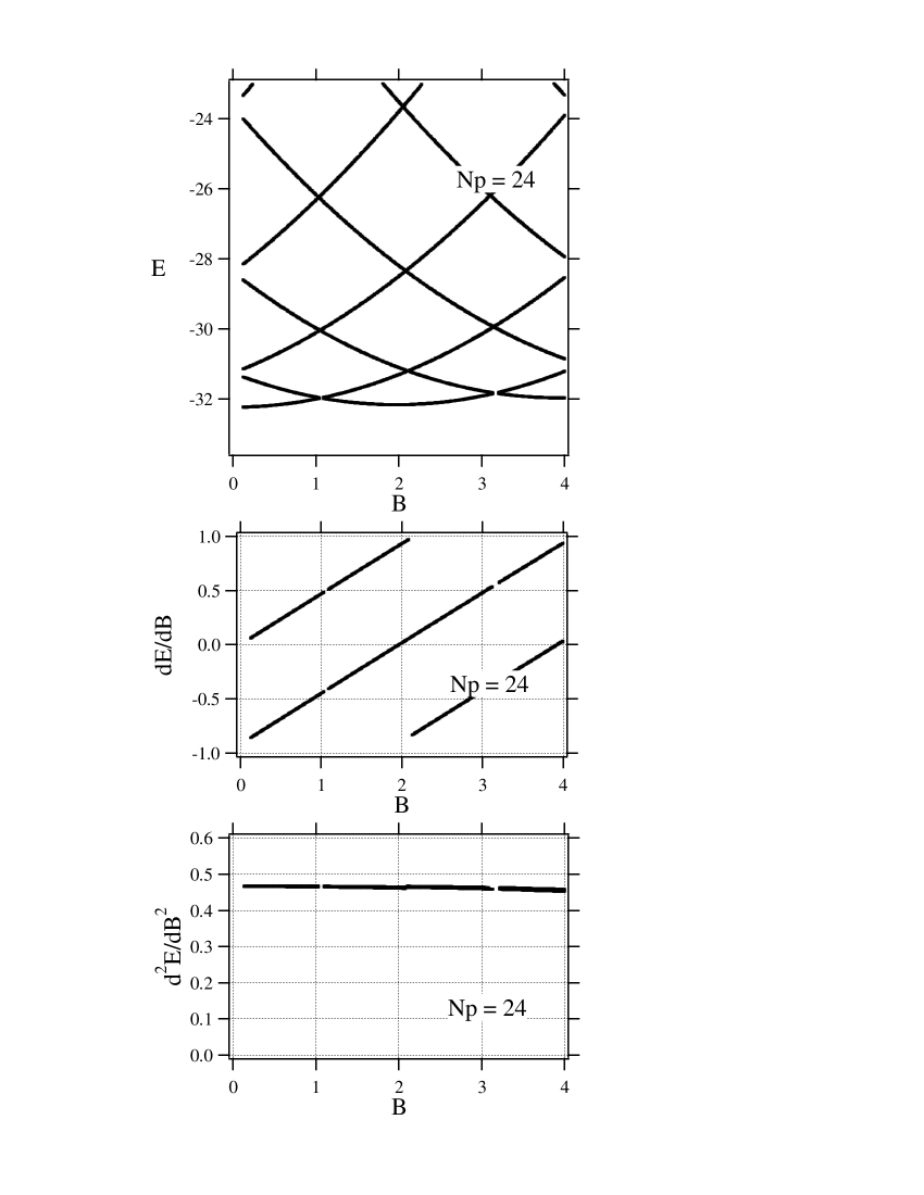
Figure 2: The energy spectra of a quantum particle on 2-dimensional plane with $Np$ delta function of strength parameter $\alpha=-1$ placed equidistantly on a ring of radius $R=1$ with perpendicular magnetic field of constant strength $B$.

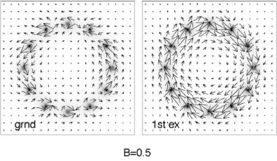
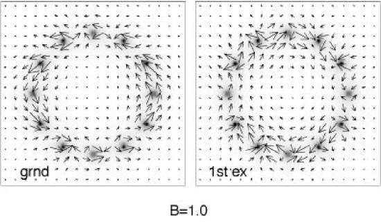
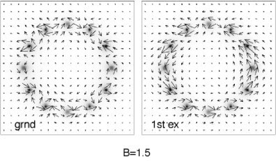
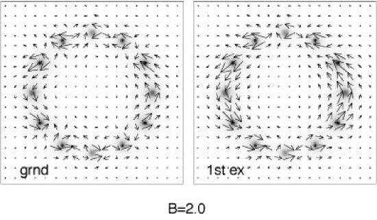
Figure 3: Profile of probability current for $Np=12$ delta-functions of strength parameter $\alpha$ placed equidistantly on a ring of radius $R=1$ and subjected to perpendicular magnetic field of constant strength $B=0.5$, $B=1.0$, $B=1.5$ and $B=2.0$.

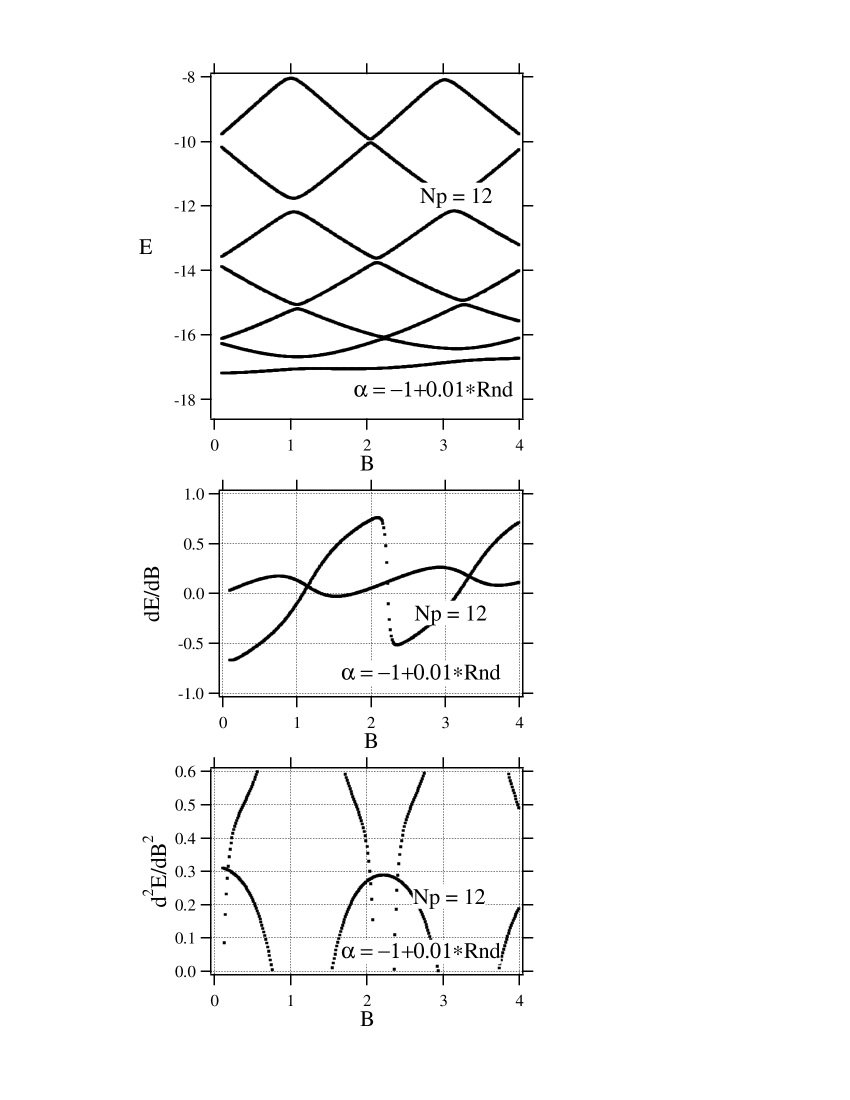
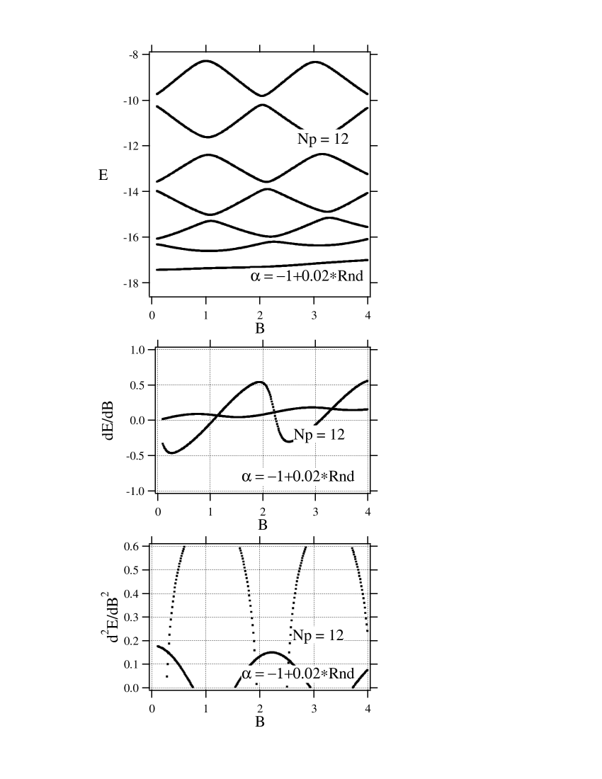
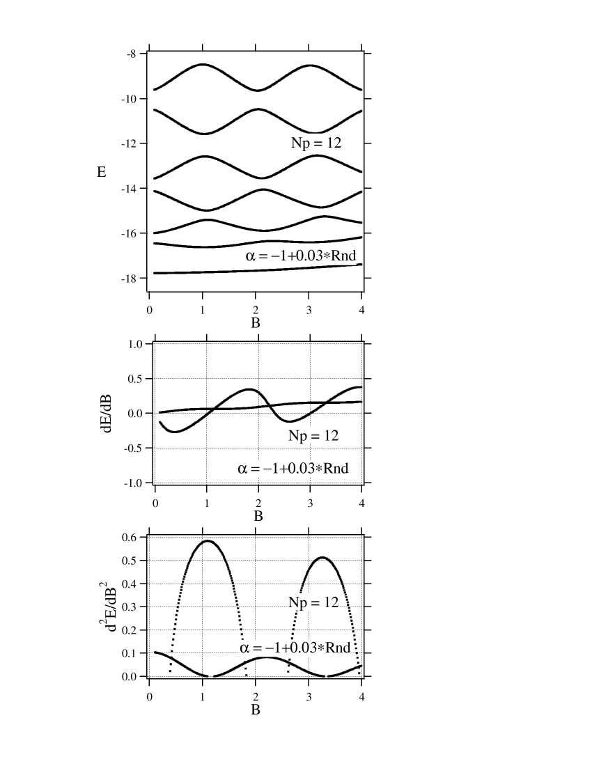
Figure 4: The energy spectra of a quantum particle on 2-dimensional plane with $Np$ delta function of fluctuating strength parameter $\alpha=-1+\Delta\alpha$ placed equidistantly on a ring of radius $R=1$ with perpendicular magnetic field of constant strength $B$.

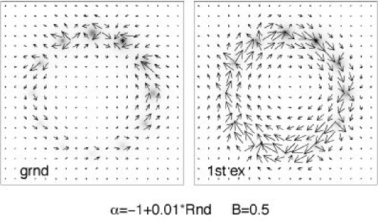
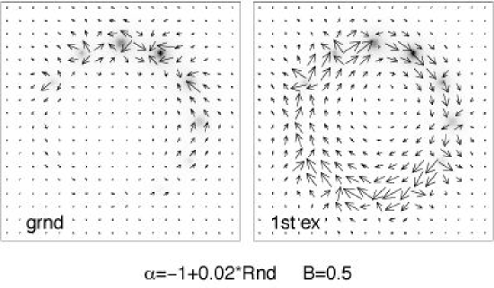
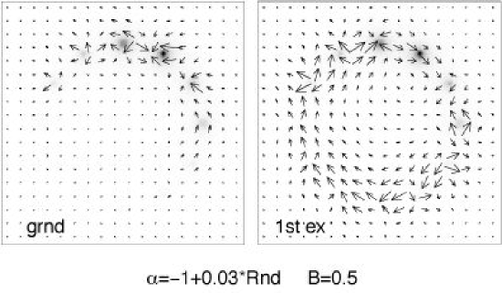
Figure 5: Profile of probability current for $Np=12$ delta-functions of fluctuating strength parameter $\alpha=-1+\Delta\alpha$ placed equidistantly on a ring of radius $R=1$ and subjected to perpendicular magnetic field of constant strength $B=0.5$.

References

- [AS] M.S. Abramowitz, I.A. Stegun, eds.: Handbook of Mathematical Functions, Dover, New York 1965.
- [AGHH] S. Albeverio, F. Gesztesy, R. Høegh-Krohn, H. Holden: Solvable Models in Quantum Mechanics, Springer, Heidelberg 1988.
- [BP] S. de Bièvre, J.V. Pulé: Propagating edge states for a magnetic Hamiltonian, Math. Phys. Electr. J. 5, no. 3 (1999).
- [CGR] H.-F.Cheng, Y.Gefen, E.K.Riedel, W.-H.Shih: Persistent currents in small one-dimensional metal rings, Phys.Rev. B37 (1988), 6050-6062.
- [CS] T.Cheon, T.Shigehara: Wave chaos in quantum billiards with a small but finite-size scatterer, Phys. Rev. E54 (1996), 1321-1331.
- [CS2] T.Cheon, T.Shigehara: Scale anomaly and quantum chaos in the billiard with pointlike scatterers, Phys. Rev. E54 (1996), 3300-3303.
- [CWB] V. Chadrasekhar, R.A. Web, M.J. Brady, M.B. Ketchen, W.J. Gallagher, A. Kleinsasser: Magnetic respense of a single, isolated gold loop, Phys. Rev. Lett. 67 (1991), 3578-3581.
- [DO] Yu.N. Demkov, V.N. Ostrovsky: Zero-Range Potentials and Their Applications in Atomic Physics, Plenum, New York 1988.
- [DMM] V.V. Dodonov, I.A. Malkin, V.I. Man’ko: The Green function of the stationary Schrödinger equation for a particle in a uniform magnetic field, Phys. Lett. A51 (1975), 133-134.
- [EJK] P. Exner, A. Joye, H. Kovařík: Edge currents in the absence of edges, Phys. Lett. A264 (1999), 124-130.
- [EŠ] P. Exner, P. Šeba: Point interactions in dimension two and three as models of small scatterers, Phys. Lett. A222 (1996), 1-4.
- [FGW] J. Fröhlich, G.M. Graf, J. Walcher: On the extended nature of edge states of quantum Hall Hamiltonians, Ann. H. Poincaré 1 (2000), 405-442.
- [FM] Ch. Ferrari, N. Macris: Intermixture of extended edge and localized bulk energy levels in macroscopic Hall systems, math-ph/0011013.
- [GHŠ] F. Gesztesy, H. Holden, P. Šeba: On point interactions in magnetic field systems, in Schrödinger Operators, Standard and Non-Standard, World Scientific 1989; pp. 147-164.
- [Ha] B.I. Halperin: Quantized Hall conductance, current carrying edge states, and the existence of extended states in two-dimensional disordered potential, Phys. Rev. B25 (1982), 2185-2190.
- [MS] A.H. MacDonald, P. Středa: Quantized Hall effect and edge currents, Phys. Rev. B29 (1984), 1616-1619.
- [MMP] N. Macris, Ph.A. Martin, J.V. Pulé: On edge states in semi-infinite quantum Hall systems, J. Phys.A.: Math. Gen. 32 (1999), 1985-96.
- [Ue] T. Ueta: Boundary element method for electron transport in the presence of pointlike scatterers in magnetic field, Phys. Rev. B60 (1999), 8213-8217.
- [We] J. Weidmann: Linear Operators in Hilbert Spaces, Springer, New York 1980