Experimental study of quantum decoherence using nuclear magnetic resonance

Abstract

Quantum decoherence has been studied using nuclear magnetic resonance(NMR). By choosing one qubit to simulate environment, we examine the decoherence behavior of two quantum systems: a one qubit system and a two qubit system. The experimental results show agreements with the theoretical predictions. Our experiment schemes can be generalized to the case that the environment is composed of multiple qubits.
PACS number(s):03.67

1. INTRODUCTION

Quantum decoherence is a purely quantum-mechanical effect through which a system loses its coherence behavior by getting entangled with its environment degrees of freedom [1][2]. A real quantum system always interacts with its surrounding environment. The time evolution induced by the interaction introduces entanglement between the system and environment when the system initially lies in a superposition of states. Quantum decoherence can be viewed as the consequence of such entanglement. When the state of the system is described by the reduced density matrix through tracing over the environment degrees of freedom, decoherence makes the off-diagonal matrix elements approach 0, and leaves diagonal ones unaltered. Quantum decoherence is thought as a main obstacle for experimental implementations of quantum computation and has been widely studied in theory [3]-[5]. Some theoretical and experimental schemes have also been proposed to solve the problem of decoherence in order to fully use coherence in quantum information[6]-[8]. Myat.C.J. et al observed and studied decoherence by coupling an ion in a Paul trap to a reservoir that can be controlled. Their experimental results tested their theoretical predictions[9][10].

As a useful tool to research the microscopic world through the macroscopic signal, nuclear magnetic resonance can be used to study the fundamental problems in quantum mechanics. Besides some quantum algorithms have been implemented on NMR quantum computers, a quantum harmonic oscillator was simulated by S. Somaroo et al [11], and the complementarity was tested by X.Zhu et al [12]. In this paper, we will study quantum decoherence using NMR. Although we choose one nucleus to simulate the environment, our schemes can be generalized to the case that the environment is composed of multiple nuclei.

2. The decoherence behavior of a one qubit system

For the simplest case, we choose a sample containing two coupled spin 1/2 nuclei to implement experiments. The two nuclei are defined as qubit 1 and qubit 2 which represent the quantum system and environment, respectively. The experimental scheme is shown in Fig.1. $R(\theta)$ denotes a rotation operation for qubit 2, and $H$ denotes the Walsh-hadamard transform for qubit 1 [13]. Experiments start with the pseudo-pure initial state $|\downarrow>_{1}|\downarrow>_{2}$ by using spatial averaging[14][15], where $|\downarrow>_{i}$ (i=1 or 2) denotes the spin ’down’ state of qubit $i$. $H$ and $R(\theta)$ transform $|\downarrow>_{1}|\downarrow>_{2}$ into $(|\uparrow>_{1}-|\downarrow>_{1})(a(\theta)|\uparrow>_{2}+b(\theta)|\downarrow>_{2})/\sqrt{2}$, where $|a|^{2}+|b|^{2}=1$. After the control-not operation is applied, the system and environment lie in the entangled state described as

$$\rho_{s+e}=\left(\begin{array}[]{cccc}|a|^{2}&ab^{*}&-ab^{*}&-|a|^{2}\\ a^{*}b&|b|^{2}&-|b|^{2}&-a^{*}b\\ -a^{*}b&-|b|^{2}&|b|^{2}&a^{*}b\\ -|a|^{2}&-ab^{*}&ab^{*}&|a|^{2}\end{array}\right),$$ (1)

where a constant factor is ignored. The state of the system is represented by the reduced density matrix[16]

$$\rho_{s}=\left(\begin{array}[]{cc}1&-ab^{*}-a^{*}b\\ -a^{*}b-ab^{*}&1\end{array}\right)$$ (2)

where the off-diagonal elements describe the coherence behavior. When $\theta$ is chosen as different values, entangled states with different amount of entanglement are gotten [17]. It is clear that the coherence of the system depends on $\theta$.

Our experiments use carbon-13 labelled chloroform dissolved in d6-acetone and carbon-13 trichloroethylene(TCE) dissolved in d-chloroform as two samples. TCE’s structure is shown in Fig.2. ¹H is decoupled during the experiments. The two ¹³C nuclei are assigned as qubit 1 and qubit 2, respectively. Data are taken at controlled temperature (22${}^{0}C$) with the Bruker DRX 500 MHz spectrometer of Beijing Normal University. For chloroform, the resonance frequencies $\nu_{1}=125.76$ MHz for ¹³C, and $\nu_{2}=500.13$ MHz for ${}^{1}H$. The coupling constant $J_{12}$ is measured to be 215 Hz. For TCE, the resonance frequencies $\nu_{1}=125.7869009$MHz (117ppm in the spectrum), $\nu_{2}=\nu_{1}+903.6Hz$. The coupling constant $J_{12}=103.1$ Hz.

The pulse sequence $[\theta]_{x}^{2}-[\frac{\pi}{2}]_{x}^{1,2}-\frac{1}{4J_{12}}-[\pi]_{x}^{1,2}-\frac{1}{4J_{12}}-[\frac{\pi}{2}]_{y}^{2}$ transforms the initial state $|\downarrow>_{1}|\downarrow>_{2}$ into an entangled state. $[\theta]_{x}^{2}$ denotes a rectangular pulse along x-axis for qubit 2, and $\frac{1}{4J_{12}}$ denotes the evolution caused by the magnetic field for $\frac{1}{4J_{12}}$ when pulses are closed. In NMR experiments, the entangled state can be described by the following deviation density matrix[18]

$$\rho_{pp}=\left(\begin{array}[]{cccc}cos^{2}(\frac{\theta}{2})&sin(\frac{\theta}{2})cos(\frac{\theta}{2})&-sin(\frac{\theta}{2})cos(\frac{\theta}{2})&-cos^{2}(\frac{\theta}{2})\\ sin(\frac{\theta}{2})cos(\frac{\theta}{2})&sin^{2}(\frac{\theta}{2})&-sin^{2}(\frac{\theta}{2})&-sin(\frac{\theta}{2})cos(\frac{\theta}{2})\\ -sin(\frac{\theta}{2})cos(\frac{\theta}{2})&-sin^{2}(\frac{\theta}{2})&sin^{2}(\frac{\theta}{2})&sin(\frac{\theta}{2})cos(\frac{\theta}{2})\\ -cos^{2}(\frac{\theta}{2})&-sin(\frac{\theta}{2})cos(\frac{\theta}{2})&sin(\frac{\theta}{2})cos(\frac{\theta}{2})&cos^{2}(\frac{\theta}{2})\end{array}\right).$$ (3)

This is the case that $a=cos(\frac{\theta}{2})$, and $b=sin(\frac{\theta}{2})$ in Equation(1). By tracing $\rho_{pp}$ over the environment degrees of freedom, the state of the system is described as

$$\rho_{spp}=\left(\begin{array}[]{cc}1&-sin\theta\\ -sin\theta&1\end{array}\right),$$ (4)

where the dependence of the coherence on $\theta$ can be represented by a sine function. In the NMR spectrum, the sum of the amplitudes of the two peaks of ¹³C is proportional to the off-diagonal element in equation (4).

Fig.3a and Fig.3b show the experimental results when the sample is chosen as chloroform. When ¹³C and ¹H lie in an entangled state, the amplitudes of the two NMR peaks of ¹³C are almost equal as shown in Fig.3a, where $\theta=50.3^{\circ}$. When $\theta$ is chosen as different values, the dependence of the coherence on $\theta$ is shown in Fig.3b. The experimental data points can be fitted as a sine-shaped curve with the period $1.96\pi$. The error is about $2.0\%$. It mainly results from the imperfection of pulses. When $\theta=0$ or $\pi$, ¹³C and ¹H lie in a maximally entangled state [18]. If we ask only about the state of ¹³C, it lies in a completely mixed-state, in which the coherence completely disappears[16]. When $\theta=\pi/2$ or $3\pi/2$ , ¹³C and ¹H lie in a product state. The coherence of ¹³C is maximal. We will discuss this case in detail. If the pulse sequence $[\theta]_{x}^{2}-[\frac{\pi}{2}]_{x}^{1,2}$ is applied to the initial state $|\downarrow>_{1}|\downarrow>_{2}$, ¹³C and ¹H are still in a product state. The spectrum of ¹³C is shown in Fig.4a, where $\theta=50.3^{\circ}$. The amplitudes of two peaks varies versus $\theta$ shown in Fig.4b, in which they are marked by ’$\triangle$’ and ’$\bigcirc$’,respectively. Nevertheless, their sum, which is corresponding to the coherence of the system, is independent of $\theta$ as shown by the line marled by ’*’ in Fig.4b.

Experimental results of TCE are shown by Fig.5a and Fig.5b. A carbon spectrum is shown in Fig.5a when $\theta=27^{\circ}$. The dependence of the coherence on $\theta$ is shown in Fig.5b. The period of the sine-shape curve is $1.83\pi$. The error is about $8.5\%$. Because the difference of the two ¹³C nuclei in TCE is much less than the difference of ¹³C and ¹H in chloroform, the selective pulses used in the latter experiment are less perfect than the former experiment. The error is larger when the sample is changed to TCE.

Our scheme can be generalized to the case that the environment is composed of $N(N>1)$ qubits. The quantum network is shown in Fig.6. For convenience, we set the rotation operation as the same form $R(\theta)$. After the system gets entangled with qubits in environment one by one, its state is represented as

$$\rho_{spp}=\left(\begin{array}[]{cc}1&-sin^{N}\theta\\ -sin^{N}\theta&1\end{array}\right).$$ (5)

When $N\rightarrow\infty$, the coherence approach 0, if $sin\theta\neq\pm 1$. In our generalized scheme, the qubits in environments are independent. We call this mode ”ideal gas” mode. The result above is in agreement with the one which is gotten by harmonic oscillator mode in theory [3].

3.The decoherence behavior of a two qubit system in an entangled state

If a two qubit system lies in an entangled state, the off-diagonal elements in its density matrix also represent the coherence. We choose carbon 13-labelled trichloroethylene dissolved in d-chloroform as a sample. The two ¹³C nuclei, which are defined as qubit 1 and qubit 2, are assigned as the system, and the ¹H, which is defined as qubit 3, is assigned as environment. The influence of the other nuclei can be ignored. The pseudo-pure initial state $|\downarrow>_{1}|\downarrow>_{2}$ is also prepared by spatial averaging [11]. ¹H is decoupled until the entangled state of the system is prepared. We choose composite pulse decoupling, and NOE can be ignored due to the short decoupling time. The following pulse sequence $[\frac{\pi}{2}]_{x}^{1,2}-\frac{1}{4J_{12}}-[\pi]_{x}^{1,2}-\frac{1}{4J_{12}}-[\frac{\pi}{2}]_{y}^{2}$ transforms $|\downarrow>_{1}|\downarrow>_{2}$ into a basis entangled state [18]

$$\rho_{s}(0)=I_{x}^{1}I_{x}^{2}-I_{z}^{1}I_{z}^{2}-I_{y}^{1}I_{y}^{2},$$ (6)

where $I_{x}^{k}$, $I_{y}^{k}$ and $I_{z}^{k}(k=1,2)$ are respectively the matrices for the three components of the angular momentum of the spins. As soon as the system lies in the entangled state, the decoupling pulses are closed. The system and environment will evolute in the magnetic field. In the rotating frame, the Hamitonian is represented as

$$H=\Delta\omega_{12}I_{z}^{1}+\Delta\omega_{32}I_{z}^{3}+2\pi J_{12}I_{z}^{1}I_{z}^{2}+2\pi J_{23}I_{z}^{2}I_{z}^{3}+2\pi J_{13}I_{z}^{1}I_{z}^{3}$$ (7)

where $\omega_{i}/2\pi(i=1,2,3)$ are the resonance frequencies of spins 1,2, and 3, $\Delta\omega_{12}=\omega_{1}-\omega_{2}$, $\Delta\omega_{32}=\omega_{3}-\omega_{2}$, and $\hbar$ is set to 1. We choose $\omega_{2}/2\pi$ as the frequency of the rotating frame. By applying a hard (nonselective) pulse $[\pi]_{x}^{1,2,3}$ in the middle of an evolution period t, the chemical shift evolution during this period can be refocused [20][21], so that the system in the entangled state evolutes under

$$H_{eff}=2\pi J_{12}I_{z}^{1}I_{z}^{2}+2\pi J_{23}I_{z}^{2}I_{z}^{3}+2\pi J_{13}I_{z}^{1}I_{z}^{3},$$ (8)

where the last two terms describe the interaction between the system and environment. Only these two terms cause the system to evolute, because entangled basis states are the eigenstates of $I_{z}^{1}I_{z}^{2}$ [19]. After evolution time t, by tracing over the environment degrees of freedom, the state of the system can be represented as

$$\rho_{s}(t)=\left(\begin{array}[]{cccc}-\frac{1}{2}&0&0&cos(\varphi_{13}+\varphi_{23})\\ 0&\frac{1}{2}&0&0\\ 0&0&\frac{1}{2}&0\\ cos(\varphi_{13}+\varphi_{23})&0&0&-\frac{1}{2}\end{array}\right),$$ (9)

where $\varphi_{13}=\pi J_{13}t$, and $\varphi_{23}=\pi J_{23}t$. In NMR experiments, this equation is equivalent to the following one

$$\rho_{s}(t)=\left(\begin{array}[]{cccc}1&0&0&-cos(\varphi_{13}+\varphi_{23})\\ 0&0&0&0\\ 0&0&0&0\\ -cos(\varphi_{13}+\varphi_{23})&0&0&1\end{array}\right)$$ (10)

The off-diagonal elements are called double quantum coherence, which can be observed through a readout pulse $[\frac{\pi}{2}]_{x}^{2}$ which transforms the system into the state represented as

$$\rho_{sr}(t)=\left(\begin{array}[]{cccc}0&i&-icos(\varphi_{13}+\varphi_{23})&cos(\varphi_{13}+\varphi_{23})\\ -i&0&cos(\varphi_{13}+\varphi_{23})&icos(\varphi_{13}+\varphi_{23})\\ icos(\varphi_{13}+\varphi_{23})&cos(\varphi_{13}+\varphi_{23})&0&-i\\ cos(\varphi_{13}+\varphi_{23})&-icos(\varphi_{13}+\varphi_{23})&i&0\end{array}\right).$$ (11)

The coherence behavior can be observed in the NMR spectrum.

Experimental data are also taken at controlled temperature (22${}^{0}C$) with a Bruker DRX 500 MHz spectrometer. The coupling constants $J_{12}=103.1$Hz, $J_{23}=201.3$Hz, and $J_{13}=9.23$Hz. ¹H is again decoupled during recording the FID signal in order to simplify the spectrum. From the view of quantum mechanics, decoupling also can be thought as the process of tracing over the environment degrees of freedom to get the reduced density matrix of the system. We will discuss this point in detail in another paper. Fig.7a is the carbon spectrum through the readout pulse $[\frac{\pi}{2}]_{x}^{2}$ when the evolution time is 3.50ms. Fig.7b shows that the amplitude of the left peak of C1(see Fig.2) in the spectrum varies versus the evolution time. The experimental data points can be fitted as function $5.8cos(2\pi t/T)$, where $T=8.72ms$. In theory, $T=9.50$ms. The error is about $8.2\%$. It mainly results from the imperfection of pulses, and the effect of decoherence which cannot be controlled.

If environment is composed of multiple qubits, the interaction between the system and environment is represented as

$$H_{i}=\sum_{k=3}^{N+2}(2\pi J_{1k}I_{z}^{1}I_{z}^{k}+2\pi J_{2k}I_{z}^{2}I_{z}^{k}).$$ (12)

Under the evolution induced by $H_{i}$, the state of the system is described as

$$\rho_{12}(t)=I_{x}^{1}I_{x}^{2}\prod_{k=3}^{N+2}cos(\varphi_{1k}+\varphi_{2k})-I_{z}^{1}I_{z}^{2}-I_{y}^{1}I_{y}^{2}\prod_{k=3}^{N+2}cos(\varphi_{1k}+\varphi_{2k}),$$ (13)

where $\varphi_{1k}=\pi J_{1k}t$, and $\varphi_{2k}=\pi J_{2k}t$. If $N\rightarrow\infty$, the coherence usually approachs to 0 very fast,if $t\neq 0$. The decoherence of the system is also caused by the entanglement between the system and environment.

4. Conclusion

In our experiments, we examine quantum decoherence of two systems by two experimental schemes. For the one qubit system, the entanglement between the system and environment is realized a quantum network. For the two qubit system, such entanglement results from the evolution induced by the interaction between the system and environment. Although the two schemes seem different, the interaction is their common prerequisite. We can get the results when the environment is composed of multiple qubits by generalizing our schemes. It is unnecessary to consider the state of the environment. In fact, we usually cannot describe the state of environment clearly. Through the entanglement between the system and environment, the environment degrees of freedom are introduced into the state of the system. Decoherence is the result of tracing over such degrees of freedom. If real environment consists of multiple particles each of which has more than two degrees of freedom, our results are still correct.

Acknowledgements

This work was partly supported by the National Nature Science Foundation of China. We are also grateful to Professor Shouyong Pei of Beijing Normal University for his helpful discussions on the theories in quantum mechanics and Miss Jinna Pan and for her help during experiments.

Figure Captions

1. Quantum network used to study the decoherence behavior of a one qubit system. Qubit 1 and qubit 2 are defined as the system and environment, respectively. $H$ denotes the Walsh-hadamard transform, and $R(\theta)$ is a rotation for qubit 2.

2. The structure of trichloroethylene. The two ${}^{13}C$ nuclei are assigned as qubit 1 and qubit 2, respectively.

3. The experimental results when ¹³C and ¹H of chloroform lie in entangled states. Fig.3a is the carbon spectrum when $\theta=50.3^{\circ}$. Fig.3b shows the dependence of the coherence on $\theta$. The experimental data points can be fitted as a sine-shaped curve with the period $1.96\pi$.

4. The experimental results when ¹³C and ¹H of chloroform lie in product states. Fig.4a is the carbon spectrum when $\theta=50.3^{\circ}$. The amplitudes of two peaks varies versus $\theta$ are also shown in Fig.4b, in which they are marked by ’$\triangle$’ and ’$\bigcirc$’, respectively. Their sum, which is corresponding to the coherence of the system, is independent of $\theta$ as shown by the line marked by ’*’.

5. The experimental results when two ¹³C nuclei of trichloroethylene lie in entangled states. Fig.5a is the carbon spectrum when $\theta=27^{\circ}$. Fig.5b shows the dependence of the coherence on $\theta$. The experimental data points can be fitted as a sine-shaped curve with the period $1.83\pi$. ¹H is decoupled during the whole experiments.

6. The generalized experimental scheme when environment is composed of qubit 2, qubit 3, …, and qubit N+1. Qubit 1 denotes the system.

7. The experimental results when the two ¹³C nuclei of trichloroethylene in the entangled state evolute under $H_{eff}$(see the text). Fig.7a is the carbon spectrum through the readout pulse $[\frac{\pi}{2}]_{x}^{2}$ when the evolution time is 3.50ms. Fig.7b shows that the amplitude of the left peak of C1(shown in Fig.2) varies versus the evolution time which is denoted as t. The experimental data points can be fitted as function $5.8cos(2\pi t/T)$, where $T=8.72ms$. ¹H is decoupled during recording the FID signal.

1

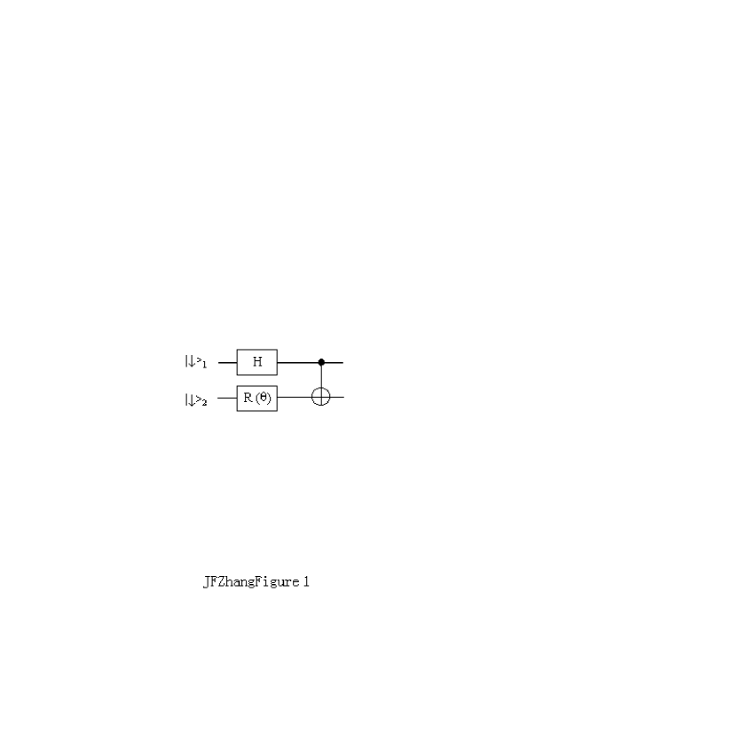
Figure 1:

2

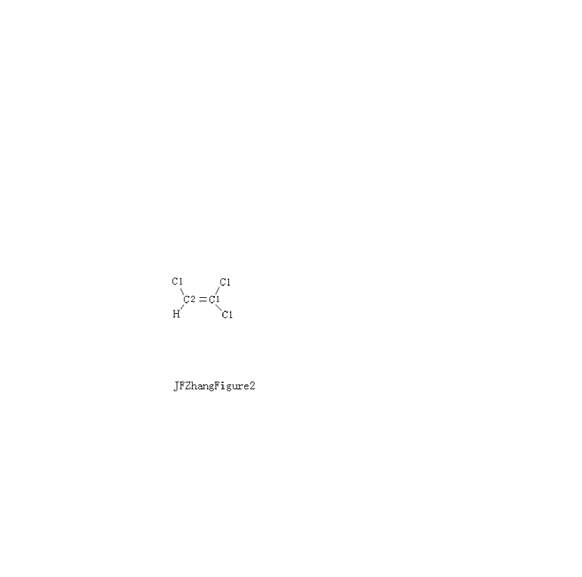
Figure 2:

3

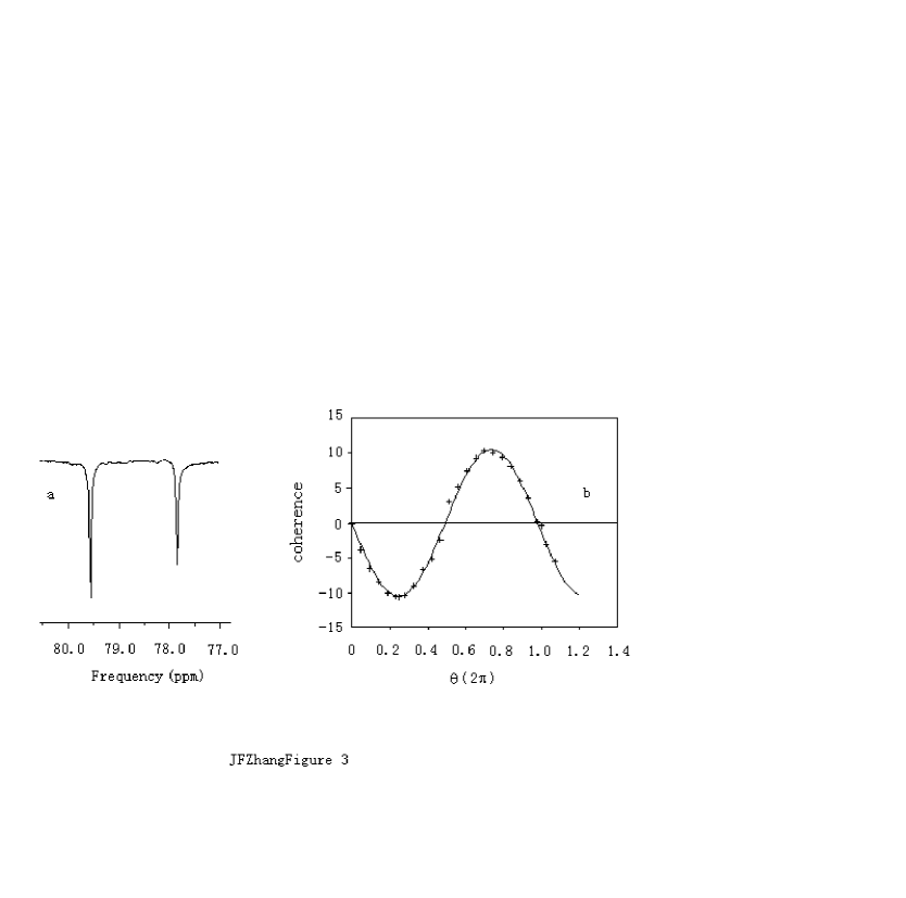
Figure 3:

4

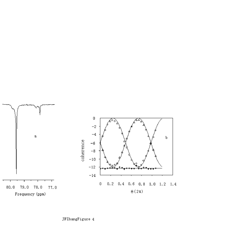
Figure 4:

5

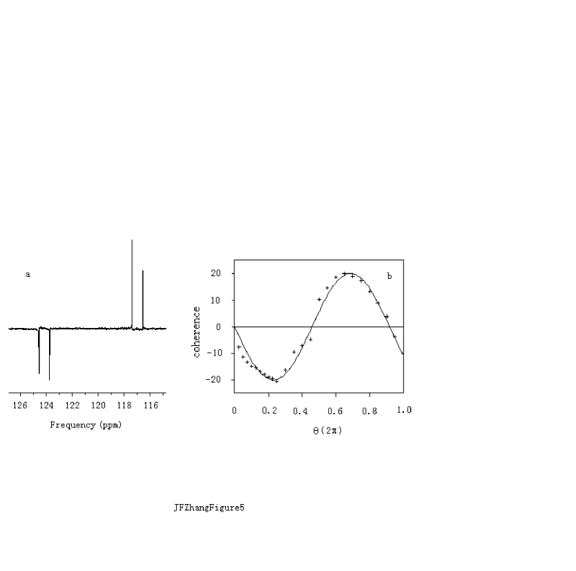
Figure 5:

6

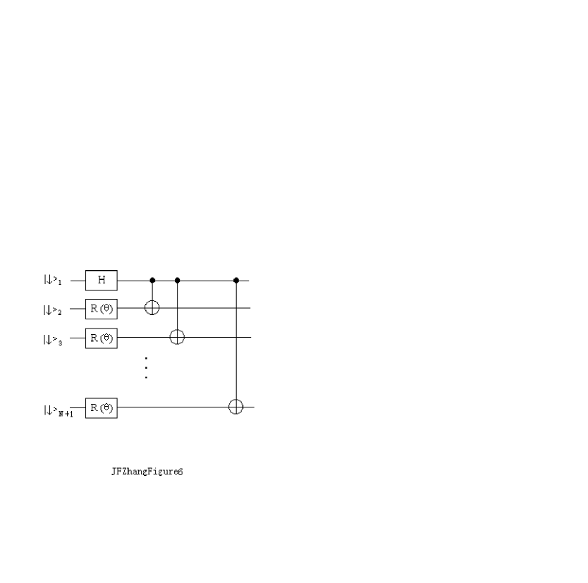
Figure 6:

7

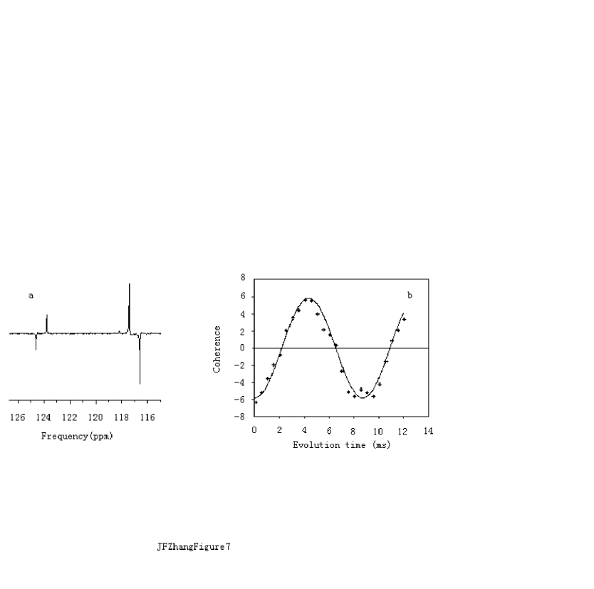
Figure 7:

References

- [1] L.Viola, E.Knill,and S.Lloyd, Phys.Rev.Lett. 82,2417(1998)
- [2] A.K.Ekert,G.M.Palma,and K.A.Suominen,in The Physics of quantum Information,edited by D. Bouwmeester, A.Ekert, and A. Zeilinger. (Springer,Berlin Heidelberg,2000)pp.222-227.
- [3] C.Sun,X.Yi,D.Zhou,and S.Yu, Problems of quantum decoherence in The new progress in Quantum Mechanics edited by J.Zeng,and S.Pei.(Beijing University pressing house,2000)pp.59-130(in chinese)
- [4] S.J.van Enk,O.Hirota,quant-ph/0012086; Phys.Rev.A,64,022313(2001)
- [5] G.M.Palma, K.A. Suominen,and A.K.Ekert,Proc.R.Soc.Lond. A,452,567(1996)
- [6] L.Viola, S.Lloyd, and E.Knill, Phys.Rev.Lett. 83,4888(1999)
- [7] D.G.Cory,M.D.Price,W.Mass,E.Knill,R.Laflamme,W.H. Zurek,T.F.Havel, and S.S.somaroo.Phys.Rev.Lett. 81,2152(1998)
- [8] E.Knill,R. Laflamme,R.Martinez,and C.Negrevergne.Phys.Rev.Lett. 86,5811(2001)
- [9] C.J.Myatt, B.E.King, Q.A.Turchette,C.A.Sackett, D.Kielpinski,W.M.Itano,C.Monroe, and D.J.Wineland,Nature,403,269(2000)
- [10] W.P.Schleich,Nature,403,256(2000)
- [11] S.Somaroo,C.H.Tseng,T.F.Havel,R.Laflamme,and D.G.Cory, 82,5381(1999)
- [12] X.Zhu,X.Fang,X.Peng,M.Feng,K.Gao,and F.Du,e-print quant-ph/0011094
- [13] A.Steane,Rep.Prog.Phys,61,117(1998)
- [14] D.G.Cory,M.D.Price,and T.F.Havel,Physica D,120,82(1998)
- [15] J.Zhang, Z.Lu, L.Shan, and Z.Deng,Phys. Rev.A,65,0343XX(2002) (in pressing)
- [16] C.D.Cantrell,and M.O.Scully,Phys.Rep,43,501(1978)
- [17] C.H.Bennett,D.P.DiVincenzo,J.A.Smolin, and W.K.Wootters, Phys. Rev.A,54,3824(1996)
- [18] I. L.Chuang, N.Gershenfeld,M.G.Kubinec and D.W.Leung, Proc.R.Soc.Lond.A 454,447 (1998)
- [19] http://www.theory.caltech.edu/ preskill/ph229
- [20] N.Linden,.Kupe,and R.Freeman,Chem.Phys.Lett,311,321(1999)
- [21] J.Kim,J.S.Lee,and S.Lee, Phys.Rev.A,62,022312(2000)