Non-Markovian stochastic Schrödinger equations: Generalization to real-valued noise using quantum measurement theory

Abstract

Do stochastic Schrödinger equations, also known as unravelings, have a physical interpretation? In the Markovian limit, where the system on average obeys a master equation, the answer is yes. Markovian stochastic Schrödinger equations generate quantum trajectories for the system state conditioned on continuously monitoring the bath. For a given master equation, there are many different unravelings, corresponding to different sorts of measurement on the bath. In this paper we address the non-Markovian case, and in particular the sort of stochastic Schrödinger equation introduced by Strunz, Diósi, and Gisin [Phys. Rev. Lett. 82, 1801 (1999)]. Using a quantum measurement theory approach, we rederive their unraveling which involves complex-valued Gaussian noise. We also derive an unraveling involving real-valued Gaussian noise. We show that in the Markovian limit, these two unravelings correspond to heterodyne and homodyne detection respectively. Although we use quantum measurement theory to define these unravelings, we conclude that the stochastic evolution of the system state is not a true quantum trajectory, as the identity of the state through time is a fiction.

I Introduction

In nature, a quantum system is most likely found in an entanglement with at least one other quantum system. An example of this is a two level atom (TLA) immersed in an environment of harmonic oscillators (the electromagnetic field). This type of quantum system, a small system interacting with a larger system (the bath) is called an open quantum system Car93 . The system-bath interaction causes the two systems to entangle, resulting in a combined state $|{\Psi(t)}\rangle$ whose evolution can be theoretically determined by the Schrödinger equation. However, due to the many degrees of freedom of the bath, this is generally impractical and it is best to describe the system (TLA) by the reduced state $\rho_{\rm red}(t)$. The evolution of $\rho_{\rm red}(t)$ is found by averaging the outer product of the Schrödinger equation over all the possible bath states,

$$\rho_{\rm red}(t)={\rm Tr}_{\rm field}[|{\Psi(t)}\rangle\langle{\Psi(t)}|].$$ (1)

Under the Born-Markov approximations Gar91 it is possible to obtain a closed equation for $\rho_{\rm red}(t)$. For mathematical consistency, this should be of the Lindblad form Lin76 . If there is a single Lindblad operator $\hat{L}$ (such as the lowering operator for the system) then this is an equation of the form

$$\dot{\rho}_{\rm red}(t)=-i[\hat{H},\rho_{\rm red}(t)]+\gamma{\cal D}[\hat{L}]\rho_{\rm red}(t),$$ (2)

where $\hat{H}$ is the Hamiltonian and

$${\cal D}[\hat{L}]\rho_{\rm red}=\hat{L}\rho_{\rm red}\hat{L}^{\dagger}-\mbox{$\frac{1}{2}$}\hat{L}^{\dagger}\hat{L}\rho_{\rm red}-\mbox{$\frac{1}{2}$}\rho_{\rm red}\hat{L}^{\dagger}\hat{L}.$$ (3)

However this is only an approximation, in the non-Markovian situation in general one can not solve $\rho_{\rm red}(t)$ or $|{\Psi(t)}\rangle$ analytically, so $\rho_{\rm red}(t)$ is difficult to determine.

A breakthrough in solving this problem was achieved with the development of non-Markovian stochastic Schrödinger   equations (SSEs). These stochastic differential equations for a state vector were first introduced for Markovian open quantum systems in mathematical physics Dio88 ; Dio88b ; Bel88 ; BelSta92 ; Bar90 ; Bar93 ; GisPer92 ; GisPer92b ; GisPer93 and then independently in quantum optics Car93 ; DalCasMol92 ; GarParZol92 . This approach has subsequently been generalized to deal with non-Markovian systems Ima94 ; Str96 ; JacCol00 ; Cre00 ; Dio96 . In this paper we will follow the approach of Diósi, Strunz and Gisin (DSG) Dio96 ; DioStr97 ; DioGisStr98 ; StrDioGis99 . In their approach, the system state vector $|{\psi_{z}({t})}\rangle$ depends upon some (not necessarily white) noise $z(t)$, which is drawn from some probability distribution. The SSE has the property that when the outer product of $|{\psi_{z}({t})}\rangle$ is averaged over all the possible $z(t)$ one obtains $\rho_{\rm red}$(t). That is,

$$\rho_{\rm red}(t)={\rm E}[|{\psi_{z}({t})}\rangle\langle{\psi_{z}({t})}|],$$ (4)

where E[…] denotes an ensemble average over all possible $z(t)$’s.

In cases where an exact non-Markovian SSE can be derived, it is also possible to find an exact solution for $\rho_{\rm red}(t)$ by other means. A key advantage of non-Markovian SSEs lies in the cases where no exact solution is possible. In this case approximations must be made in either approach. The advantage of the SSE approach is that the ensemble average $\rho_{\rm red}(t)$ is, by construction, guaranteed to be a positive operator. This fundamental property of a state matrix is not guaranteed by other approximate equations for $\rho_{\rm red}(t)$. This is true even in in the Markov limit; quantum Brownian motion is a case in point StrDioGisYu99 . The other advantage of the SSE approach in general is that it allows the evolution of large systems to be simulated numerically. This was the original motivation for their introduction in quantum optics DalCasMol92 ; GarParZol92 .

Leaving aside the potential usefulness of SSEs, one may ask the question: is there a physical interpretation for the solution of an SSE, or is it simply a numerical tool for finding $\rho_{\rm red}(t)$? In the Markovian limit, that is when the master equation has the form Eq. (2), the answer is yes. The solution to the SSE, termed by Carmichael is a quantum trajectory Car93 , it can be interpreted as the state of the system conditioned on the measurement results obtained by continuously monitoring the bath WisMil93 . For the Markovian case, different sorts of SSEs exist. They may involve jumps or diffusion, and are termed different unravelings of the master equation Car93 . These different unravelings correspond to different detection schemes, such as photon counting Car93 ; DalCasMol92 ; GarParZol92 , homodyne Car93 ; WisMil93 ; WisMil93c , and heterodyne WisMil93c detection. Other generalizations Wis96 ; JacColWal99 ; GamWis01 ; WarWisMab01 have also been investigated.

In this paper we will investigate the question of physical interpretation of non-Markovian diffusive SSEs of Diosi, Strunz and Gisin (DSG) Str96 ; Dio96 ; DioStr97 ; DioGisStr98 ; StrDioGis99 . We will show that quantum measurement theory (QMT) does give meaning to the $|{\psi_{z}({t})}\rangle$ at any particular time, $t$. However, the linking of the state $|{\psi_{z}({t})}\rangle$ at different times to make a trajectory appears to be a convenient fiction. We also show that the theory of DSG can be generalized by considering different sorts of measurements (unravelings) on the bath. We use our approach to define two different unravelings. The first results in DSG SSEs, with complex-valued noise $z(t)$. In the Markovian limit this unraveling corresponds to heterodyne detection. The second, which can only be defined for some system-bath couplings, has real-valued noise and has homodyne detection as its Markovian limit.

II System dynamics and Quantum Measurement Theory.

II.1 Schrödinger Equation for the combined system

With $\hbar=1$, a system interacting with a reservoir of harmonic oscillators has the total Hamiltonian

$$\hat{H}_{\rm tot}=\hat{H}_{0}+\hat{H}+\hat{H}_{\rm bath}+\hat{V}.$$ (5)

Here the system Hamiltonian has been split into $\hat{H}_{0}$ (the action of which is described later) and $\hat{H}$ (the remainder). The Hamiltonian for the bath is

$$\hat{H}_{\rm bath}=\sum_{k}\omega_{k}\hat{a}_{k}^{\dagger}\hat{a}_{k},$$ (6)

where $k$ labels the modes of the bath, $\hat{a}_{k}$ and $\omega_{k}$ are the lowering operator and angular frequency of the $k^{\rm th}$ mode respectively. We assume the interaction Hamiltonian to have the form

$$\hat{V}=i(\hat{L}\hat{b}^{\dagger}-\hat{b}\hat{L}^{\dagger}),$$ (7)

where $\hat{L}$ is a system operator and where we have define the bath lowering operators $\hat{b}$ as $\hat{b}=\sum_{k}g_{k}\hat{a}_{k}$. That is, the coupling amplitude of the $k^{\rm th}$ mode to the system is $g_{k}$.

The Schrödinger equation for the combined state is

$$d_{t}|{{\Psi}(t)}\rangle=-{i}\hat{H}_{\rm tot}|{\Psi(t)}\rangle,$$ (8)

which can equivalently be written as

$$|{\Psi(t)}\rangle=U(t,0)|{\Psi(0)}\rangle,$$ (9)

where $U(t,0)$ is called the unitary evolution operator. Defining a unitary evolution operator for the ‘free’ system and bath as

$$U_{0}(t,0)=e^{-i(\hat{H}_{0}+\hat{H}_{\rm bath})(t-0)}.$$ (10)

We can write $U(t,0)$ as $U(t,0)=U_{0}(t,0)U_{\rm int}(t,0)$, where $U_{\rm int}(t,0)$ is the unitary evolution operator that describes the total evolution with the free dynamics removed.

We can then define an interaction picture state as

$$|{\Psi_{\rm int}(t)}\rangle=U_{\rm int}(t,0)|{\Psi(0)}\rangle,$$ (11)

which obeys

$$d_{t}|{{\Psi}_{\rm int}(t)}\rangle=-{i}{\Bigl{(}}\hat{H}_{\rm int}(t)+\hat{V}_{\rm int}(t){\Bigr{)}}|{\Psi_{\rm int}(t)}\rangle.$$ (12)

The Hamiltonians in the interaction picture are

$$\hat{H}_{\rm int}(t) = U_{0}^{\dagger}(t,0)\hat{H}U_{0}(t,0),$$ (13)

and

$$\hat{V}_{\rm int}(t) = i{\Bigl{(}}\hat{b}_{\rm int}^{\dagger}(t)\hat{L}_{\rm int}(t)-\hat{b}_{\rm int}(t)\hat{L}_{\rm int}^{\dagger}(t){\Bigr{)}},$$ (14)

where

$$\hat{b}_{\rm int}(t) = \sum_{k}g_{k}\hat{a}_{k}e^{-i\omega_{k}t},$$ (15)

$$\hat{L}_{\rm int}(t) = \hat{L}e^{-i\omega_{0}t}.$$ (16)

Here we have finally restricted $\hat{H}_{0}$ to be such that $\hat{L}$ in the interaction picture simply rotates in the complex plane as indicated in Eq. (16). The interaction picture can be viewed as moving the time dependencies due to the free bath and system dynamics from the state to the operators. Unless otherwise stated the rest of this paper will be in the interaction picture and thus we will drop the subscripts ‘int’.

II.2 QMT and Conditional System States

In open quantum systems a measurement is always perform on the bath. Due to the entanglement between the bath and the system the measurement on the bath results in an indirect measurement of the system BraKha92 . The state of the system after the measurement is dependent on the results of the measurement, so we call this a conditional system state. To mathematically describe this (for a more detailed description see Wis96 ; BraKha92 ; Kra83 ) we define $|{\{q_{k}\}}\rangle$ as the arbitrary basis the measurement is performed in. Note that $|{\{q_{k}\}}\rangle$ does not necessarily have to be normalized. For our purposes we restrict $|{\{q_{k}\}}\rangle$ to be a state in the interaction picture with no time dependence (it will be $U_{0}^{\dagger}(t,0)|{\{q_{k}\}}\rangle$ in the Schrödinger picture). A typically example of this is a coherent bath state. This is the state (in the interaction picture) the bath (harmonic oscillators) has when driven by a classical current ScuZub97 .

In the basis $|{\{q_{k}\}}\rangle$ we can define a probability-operator-measure (POM) element, or effect, as

$$\hat{F}_{\{q_{k}\}}=|{\{q_{k}\}}\rangle\langle{\{q_{k}\}}|.$$ (17)

Here the subscript $\{q_{k}\}$ is the result of the measurement. The effect is important as it allows one to calculate the probability density of results $\{q_{k}\}$

$${P}(\{q_{k}\},t)=\langle{\Psi(t)}|\hat{F}_{\{q_{k}\}}|{\Psi(t)}\rangle.$$ (18)

If one were only interested in obtaining probabilities the effect would be all one would need. However, since we are interested in the state of the system after the measurement, we need to define a set of measurement operators. The constraint the measurement operators must obey is $\hat{F}_{\{q_{k}\}}=\hat{M}_{\{q_{k}\}}^{\dagger}\hat{M}_{\{q_{k}\}}$. For example, we can decompose the measurement operators as

$$\hat{M}_{\{q_{k}\}}=|{\{n_{k}\}}\rangle\langle{\{q_{k}\}}|,$$ (19)

where $\{n_{k}\}$ is arbitrary, and is the state the bath is left in after the measurement. Since in most detection situations a measurement results in annihilating the detected field the most natural choice for $\{n_{k}\}$ is the vacuum state $\{0_{k}\}$.

In QMT the combined state after a measurement at time $t$, which yielded results ${\{q_{k}\}}$ is BraKha92 ; Kra83

$$|{\Psi_{\{q_{k}\}}(t)}\rangle=\frac{\hat{M}_{\{q_{k}\}}|{\Psi(t)}\rangle}{\sqrt{{P}(\{q_{k}\},t)}\,}.$$ (20)

Using equation (19), with $n_{k}=0$ for all $k$, the combined state after the measurement is, $|{\Psi_{\{q_{k}\}}(t)}\rangle=|{\{0_{k}\}}\rangle|{{\psi}_{\{q_{k}\}}({t})}\rangle$, where

$$|{{\psi}_{\{q_{k}\}}({t})}\rangle=\frac{\langle{\{q_{k}\}}|\Psi(t)\rangle}{\sqrt{{P}(\{q_{k}\},t)}\,}.$$ (21)

Equation (21) is the conditional system state and we see here directly how the entanglement between the bath and the system results in the system state collapsing upon measurement of the bath. One of the properties of this conditional system state is that $\rho_{\rm red}(t)$ (equation (1)) can be written as

$$\rho_{\rm red}(t) = \int\langle{\{q_{k}\}}|\Psi(t)\rangle\langle\Psi(t)|{\{q_{k}\}}\rangle d\{q_{k}\}$$ (22)

$$= \int{P}(\{q_{k}\},t)|{{\psi}_{\{q_{k}\}}({t})}\rangle\langle{{\psi}_{\{q_{k}\}}({t})}|d\{q_{k}\}$$

$$= {\rm E}[|{{\psi}_{\{q_{k}\}}({t})}\rangle\langle{{\psi}_{\{q_{k}\}}({t})}|],$$

where E denote an average over the distribution ${P}(\{q_{k}\},t)$. From equation (4) we see that the conditional state satisfies the same requirements as a solution of a SSE. This suggests that the time derivative of equation (21), if it could be written in terms of $|{{\psi}_{\{q_{k}\}}({t})}\rangle$, could be interpreted as a SSE. One problem in determining the time-derivative is that Eq. (21) involves the probability ${P}(\{q_{k}\},t)$, which requires knowing $|{\Psi(t)}\rangle$, and, as mention earlier, this in general is indeterminable. However, this problem may be overcome using linear quantum measurement theory (LQMT).

LQMT uses the same principles as QMT except we use an ostensible distribution ($\Lambda(\{q_{k}\})$) in place of the actual probability Wis96 ; GoeGra94 . As its name suggests, the ostensible probability distribution need bear no relation to the actual probability distribution. However, it must be a proper probability distribution (non-negative, and integrating to unity), and must be non-zero wherever the actual distribution is non-zero. Using the ostensible probability distribution, the conditioned system state is

$$|{\tilde{\psi}_{\{q_{k}\}}({t})}\rangle=\frac{\langle{\{q_{k}\}}|\Psi(t)\rangle}{\sqrt{{\Lambda}(\{q_{k}\})}\,}.$$ (23)

We will call it the linear conditioned system state, because it depends linearly on the pre-measurement state $|{\Psi(t)}\rangle$, unlike Eq. (21). Since $\Lambda(\{q_{k}\})$ is not equal to the actual probability, $|{\tilde{\psi}_{\{q_{k}\}}({t})}\rangle$ will not be normalized and to signify this we use a tilde above the state. Note that this notation, following our earlier convention Wis96 ; GamWis01 , is the reverse of that used by DSG DioGisStr98 . Because it is unnormalized, the linear conditioned system state does not have a clear physical interpretation. However, it still is useful as it is easier to calculate (involving only linear equations), and we can write

$$\rho_{\rm red}(t) = \int\langle{\{q_{k}\}}|\Psi(t)\rangle\langle\Psi(t)|{\{q_{k}\}}\rangle d\{q_{k}\}$$ (24)

$$= \int{\Lambda}(\{q_{k}\})|{\tilde{\psi}_{\{q_{k}\}}({t})}\rangle\langle{\tilde{\psi}_{\{q_{k}\}}({t})}|d\{q_{k}\}$$

$$= {\rm\tilde{E}}[|{\tilde{\psi}_{\{q_{k}\}}({t})}\rangle\langle{\tilde{\psi}_{\{q_{k}\}}({t})}|],$$

where ${\rm\tilde{E}}$ denote an average using the ostensible distribution $\Lambda(\{q_{k}\})$. The condition for obtaining a linear SSE is we have to be able to write the time derivative of equation (23) in terms of only $|{\tilde{\psi}_{\{q_{k}\}}({t})}\rangle$.

A linear SSE is only really useful if it can be transformed into a nonlinear SSE for the normalized state $|{{\psi}_{\{q_{k}\}}({t})}\rangle$. To do this one requires that there exists a Girsanov transformation for the variables $\{q_{k}\}$ GatGis91 . This is a transformation that takes into account the relation between the actual probability to ostensible probability,

$${P}(\{q_{k}\},t)=\langle{\tilde{\psi}_{\{q_{k}\}}({t})}|\tilde{\psi}_{\{q_{k}\}}(t){\rangle}\Lambda({\{q_{k}\}}),$$ (25)

which follows from Eqs. (23) and (18). Specifically, the Girsanov transformation is a time-dependent transformation that changes the variables $\{q_{k}\}$ into the variables $\{{q}_{k}^{\Lambda}\}$ such that

$$\Lambda(\{q_{k}^{\Lambda}\})d\{q_{k}^{\Lambda}\}=P(\{q_{k}\},t)d\{q_{k}\}.$$ (26)

We can see the usefulness of this transformation as follows. If we normalize the unnormalized states, but keep the same ostensible distribution, then the ensemble average will not reproduce $\rho_{\rm red}(t)$:

$$\int\frac{\Lambda(\{q_{k}\})}{|\tilde{\psi}_{\{q_{k}\}}|^{2}}|{\tilde{\psi}_{\{q_{k}\}}({t})}\rangle\langle{\tilde{\psi}_{\{q_{k}\}}({t})}|d\{q_{k}\}\neq\rho_{\rm red}(t).$$ (27)

However if $\{q_{k}\}$ are chosen from the actual distribution then, of course it does:

$$\int\frac{P(\{q_{k}\},t)}{|\tilde{\psi}_{\{q_{k}\}}|^{2}}|{\tilde{\psi}_{\{q_{k}\}}({t})}\rangle\langle{\tilde{\psi}_{\{q_{k}\}}({t})}|d\{q_{k}\}=\rho_{\rm red}(t).$$ (28)

Equivalently, using the ostensible distribution for $\{q_{k}^{\Lambda}\}$,

$$\int\frac{\Lambda(\{q_{k}^{\Lambda}\})}{|\tilde{\psi}_{\{q_{k}\}}|^{2}}|{\tilde{\psi}_{\{q_{k}\}}({t})}\rangle\langle{\tilde{\psi}_{\{q_{k}\}}({t})}|d\{q^{\Lambda}_{k}\}=\rho_{\rm red}(t).$$ (29)

Note that both $\{q_{k}\}$ and $\{q_{k}^{\Lambda}\}$ appear here. This means that if we have a linear SSE, we can derive a nonlinear (‘actual’) SSE by normalizing the state

$$|{{\psi}_{\{q_{k}\}}({t})}\rangle=\frac{1}{|\tilde{\psi}_{\{q_{k}\}}|}|{\tilde{\psi}_{\{q_{k}\}}({t})}\rangle,$$ (30)

where

$${|\tilde{\psi}_{\{q_{k}\}}|}=\sqrt{\langle{\tilde{\psi}_{\{q_{k}\}}({t})}|\tilde{\psi}_{\{q_{k}\}}(t){\rangle}}\,,$$ (31)

but generating the SSE by drawing $\{q_{k}^{\Lambda}\}$ rather than $\{q_{k}\}$ from the ostensible distribution.

Now that we know how to use Eq. (30), we can calculate the time derivative of $|{{\psi}_{\{q_{k}\}}({t})}\rangle$ in terms of $|{\tilde{\psi}_{\{q_{k}\}}({t})}\rangle$. This results in

$$d_{t}|{{\psi}_{\{q_{k}\}}({t})}\rangle=\frac{1}{|\tilde{\psi}_{\{q_{k}\}}|}d_{t}|{\tilde{\psi}_{\{q_{k}\}}({t})}\rangle+|{\tilde{\psi}_{\{q_{k}\}}({t})}\rangle d_{t}\frac{1}{|\tilde{\psi}|},$$ (32)

where

$$d_{t}|{\tilde{\psi}_{\{q_{k}\}}({t})}\rangle={\partial_{t}}|{\tilde{\psi}_{\{q_{k}\}}({t})}\rangle+\sum_{k}d_{t}{q}_{k}{\partial_{q_{k}}}|{\tilde{\psi}_{\{q_{k}\}}({t})}\rangle.$$ (33)

Here we have assumed that we can define $d_{t}q_{k}$ so as to generate a $q_{k}(t)$ which ensures that Eq. (26) is always satisfied. From the above discussion, it is thus apparent that three conditions must be satisfied if Eq. (32) is to be a SSE for the system state $|{{\psi}_{\{q_{k}\}}({t})}\rangle$. These are:

1. It is possible to obtain a linear SSE, that is ${\partial_{t}}|{\tilde{\psi}_{\{q_{k}\}}({t})}\rangle$.

2. There is a Girsanov transformation $\{q_{k}^{\Lambda}\}\to\{q_{k}(t)\}$ such that an equation for $d_{t}{q}_{k}$ for all $k$ can be found explicitly.

3. Equation (32) can be written in terms of only $|{{\psi}_{\{q_{k}\}}({t})}\rangle$.

If we can satisfy all these conditions then we have a SSE which generates a state with a definite physical interpretation. The SSE generates a state at time $t$ which is of the form of Eq. (21). This is clearly the normalized state conditioned on a measurement being performed at time $t$ on the entire bath, and yielding results $\{q_{k}\}$.

It is important to note, however, that the linking of the states at earlier times to form a trajectory (which is how the SSE generates the state at time $t$) appears to be a convenient fiction. A measurement on the whole bath at time $t$ is clearly incompatible with a similar measurement at an earlier time. It is only in the Markovian limit that compatible bath measurements can be made, so that the quantum trajectory as a whole can be interpreted physically. In other words the time evolution generated by the SSE simply links together hypothetical conditioned states at different times, with different measurement results $\{q_{k}(t)\}$. The relation between the results at different times is purely mathematical, not physical. The mathematical relation comes from the time-dependent Girsanov transformation: the $q^{\Lambda}_{k}$ corresponding to the $q_{k}(t)$ are the same at all times.

III Coherent Bath Unraveling

III.1 Coherent Noise Operator

The first unraveling we consider is that associated with the bath being projected into a multitude mode coherent states, that is $|{\{q_{k}\}}\rangle=|{\{a_{k}\}}\rangle$ where

$$|{\{a_{k}\}}\rangle=\prod_{k}\frac{1}{\sqrt{\pi}\,}e^{-|a_{k}|^{2}/2}\sum_{n_{k}}\frac{a_{k}^{n_{k}}}{\sqrt{n_{k}!}\,}|{n_{k}}\rangle.$$ (34)

Note that these states are deliberately not normalized, so that the multi-mode integral of the effect $\hat{F}_{\{a_{k}\}}=|{\{a_{k}\}}\rangle\langle{\{a_{k}\}}|$ is unity. We call the resultant unraveling the ‘coherent state unraveling’. For this unraveling we define the noise operator

$$\hat{z}(t)=\hat{b}(t)e^{i\omega_{0}t}=\sum_{k}g_{k}\hat{a}_{k}e^{-i\Omega_{k}t},$$ (35)

where $\Omega_{k}=\omega_{k}-\omega_{0}$. This noise operator has the property

$$\hat{z}(t)|{\{a_{k}\}}\rangle=z(t)|{\{a_{k}\}}\rangle,$$ (36)

where $z(t)$ is the noise function, given by

$${z}(t)=\sum_{k}g_{k}{a}_{k}e^{-i\Omega_{k}t}.$$ (37)

An important property of the bath is its correlation: how the noise operator (function) at time $t$ is related to that at time $s$. This is determined by the commutator (operators) or correlation function (noise functions). For a non-Hermitian operator there are two important commutators,

$$[\hat{z}(t),\hat{z}(s)] = 0,$$ (38)

$$[\hat{z}(t),\hat{z}(s)^{\dagger}] = \alpha{(t-s)},$$ (39)

where, in the notation of DSG,

$$\alpha{(t-s)}=\sum_{k}|g_{k}|^{2}e^{-i\Omega_{k}(t-s)},$$ (40)

which we call the memory function.

The second form of correlation in defined in terms of the noise functions as ${\rm E}[z(t)z^{*}(s)]$. This depends on the probability for obtaining the results $\{a_{k}\}$ in the measurement at the two times. In linear QMT, these probabilities are given by the ostensible distribution $\Lambda(\{a_{k}\})$, which may be chosen to be time-independent. It is convenient to choose $\Lambda(\{a_{k}\})$ to be equal to the actual probability that would arise when the bath is always in the vacuum state. That is,

$${\Lambda}(\{a_{k}\})=\langle{\{0_{k}\}}|{\{a_{k}\}}\rangle\langle{\{a_{k}\}}|{\{0_{k}\}}\rangle={\pi^{-\kappa}}{e^{-\sum_{k}|a_{k}|^{2}}},$$ (41)

where $\kappa=\sum_{k}$. As will be seen later, this is appropriate if the bath is initially in this state. The correlation for the noise functions under this assumption is,

$$\tilde{{\rm E}}[{z}(t)z^{*}(s)] = \alpha{(t-s)},$$ (42)

$$\tilde{{\rm E}}[{z}(t)z(s)] = 0.$$ (43)

Note that we have used the notation discussed below Eq. (24). Thus for the special case where the ostensible probability is given by Eq. (41), the memory function is equal to the correlation of the noise functions.

III.1.1 The Markov Limit

Since one of our aims is to consider the Markovian limit of our non-Markovian SSEs (in which one obtains a genuine quantum trajectory), the Markov limit of all our main results will be presented. In the Markov limit the number of modes become continuous and the coupling constant $|g_{k}|$ becomes flat ($|g_{k}|=g$) and equal to $\sqrt{\gamma/2\pi}\,$. This allows us to write

$$\alpha{(t-s)} = \frac{\gamma}{2\pi}\int_{0}^{\infty}e^{-i(\omega-\omega_{0})(t-s)}d\omega$$ (44)

$$= \frac{\gamma}{2\pi}\int_{-\omega_{0}}^{\infty}e^{-i\Omega(t-s)}d\Omega,$$

and for optical situations (high $\omega_{0}$ situations) with little error this can be written as

$$\alpha{(t-s)}=\frac{\gamma}{2\pi}\int_{-\infty}^{\infty}e^{-i\Omega(t-s)}d\Omega=\gamma\delta{(t-s)}.$$ (45)

Therefore,

$$\tilde{\rm E}[z(t)z^{*}(s)]\,=\,[\hat{z}(t),\hat{z}(s)^{\dagger}] = \gamma\delta{(t-s)},$$ (46)

$$\tilde{{\rm E}}[{z}(t)z(s)]\,=\,[\hat{z}(t),\hat{z}(s)] = 0.$$ (47)

This implies that ostensibly $z(t)$ is a complex gaussian random variable (GRV) of mean 0 and variance $\gamma/dt$. That is, $z(t)=\sqrt{\gamma}\,\zeta(t)$, where $\zeta(t)$ is the standard complex white noise function Gar83 . These are the correct correlation function for the heterodyne noise functions Wis96 .

III.2 The Linear Stochastic Schrödinger Equations for the Coherent Unraveling

In this section we will derive the linear non-Markovian SSEs for the ostensible probability introduced above, and show that in the Markov limits it gives the linear Heterodyne SSE. We use many of the same techniques as DSG. To calculate the linear SSE we write the Schrödinger equation in terms of the noise operator, $\hat{z}(t)$

$$d_{t}|{\Psi(t)}\rangle=\Big{\{}{-i}\hat{H}(t)+\hat{z}^{\dagger}(t)\hat{L}-\hat{z}(t)\hat{L}^{\dagger}\Big{\}}|{\Psi(t)}\rangle.$$ (48)

Then by differentiating equation (23) with respect to time (with $q_{k}$ set to $a_{k}$) we obtain

$$\partial_{t}|{\tilde{\psi}_{\{a_{k}\}}({t})}\rangle = \Big{\{}{-i}\hat{H}(t)+z^{*}(t)\hat{L}\Big{\}}|{\tilde{\psi}_{\{a_{k}\}}({t})}\rangle$$ (49)

$$-\frac{\langle{\{a_{k}\}}|\hat{z}(t)\hat{L}^{\dagger}|{\Psi(t)}\rangle}{\sqrt{\Lambda({\{a_{k}\}})}\,},$$

as $\hat{H}(t)$ is a system-only operator and $\langle{\{a_{k}\}}|$ is the left-eigenstate of $\hat{z}(t)^{\dagger}$. To satisfy the condition for a linear SSE we must evaluate the last term in this equation in terms of $|{\tilde{\psi}_{\{a_{k}\}}({t})}\rangle$. To do this we use ScuZub97 ,

$$\langle{\{a_{k}\}}|\hat{a}_{k}|{\Psi(t)}\rangle=\Big{(}\frac{a_{k}}{2}+{\partial_{a^{*}_{k}}}\Big{)}\langle{\{a_{k}\}}|{\Psi(t)}\rangle$$ (50)

and

$${\partial_{a^{*}_{k}}}|{\tilde{\psi}_{\{a_{k}\}}({t})}\rangle=\frac{\partial_{a^{*}_{k}}\langle{\{a_{k}\}}|{\Psi(t)}\rangle}{\sqrt{\Lambda({\{a_{k}\}})}\,}+\frac{a_{k}}{2}|{\tilde{\psi}_{\{a_{k}\}}({t})}\rangle.$$ (51)

With these two expressions and the definition of $\hat{z}(t)$,

$$\frac{\langle{\{a_{k}\}}|\hat{z}(t)|{\Psi(t)}\rangle}{\sqrt{\Lambda({\{a_{k}\}})}\,}=\sum_{k}g_{k}e^{-i\Omega_{k}t}{\partial_{a^{*}_{k}}}|{\tilde{\psi}_{\{a_{k}\}}({t})}\rangle.$$ (52)

This allows us to write equation (49) as

$$\partial_{t}|{\tilde{\psi}_{\{a_{k}\}}({t})}\rangle = \Big{\{}{-i}\hat{H}(t)+z^{*}(t)\hat{L}-\hat{L}^{\dagger}\sum_{k}g_{k}e^{-i\Omega_{k}t}$$ (53)

$$\times{\partial_{a^{*}_{k}}}\Big{\}}|{\tilde{\psi}_{\{a_{k}\}}({t})}\rangle.$$

This is a linear equation in terms of $\{a_{k}\}$. Note that it is not really a SSE, as the final term implies that the evolution of the state $|{\tilde{\psi}_{\{a_{k}\}}({t})}\rangle$ depends not only on itself, but upon neighbouring states with different values of $\{a_{k}\}$. That is, we cannot simply choose (stochastically) a value for $\{a_{k}\}$ from the ostensible distribution and then propagate forward the system state using that value. However, we can make progress towards an equation where we can do this by rewriting the partial derivative in terms of a functional derivative. This is done by using the following relation (see for example ParYan89 ),

$${\partial_{a^{*}_{k}}}=\int_{0}^{t}\frac{\delta}{\delta z^{*}(s)}\frac{\partial z^{*}(s)}{\partial{a^{*}_{k}}}ds,$$ (54)

where $0$ is the initial time. This gives

$$\partial_{t}|{\tilde{\psi}_{z}({t})}\rangle = \Big{\{}{-i}\hat{H}(t)+z^{*}(t)\hat{L}-\hat{L}^{\dagger}\int_{0}^{t}\alpha{(t-s)}$$ (55)

$$\times\frac{\delta}{\delta z^{*}(s)}ds\Big{\}}|{\tilde{\psi}_{z}({t})}\rangle,$$

where $\alpha{(t-s)}$ is defined in equation (40). By replacing the partial derivatives by the functional derivative we have enforced the initial condition $|{\Psi(0)}\rangle=|{\{0_{k}\}}\rangle|{\psi(0)}\rangle$, This is seen as follows. At $t=0$ the functional derivative term in the above equation will have zero contribution, from the definition (54). By comparison with the corresponding term in Eq. (53), it follows that $\partial_{a^{*}_{k}}|{\tilde{\psi}_{\{a_{k}\}}({t})}\rangle|_{t=0}=0$ for all $k$. From Eq. (23) this is only possible if the system and bath states initially (at time $0$) factorize, and if $\Lambda(\{a_{k}\})=|\langle\{a_{k}\}|\psi_{\rm bath}\rangle|^{2}$. From our choice (41) of ostensible probability, this enforces $|{\psi_{\rm bath}}\rangle=|{\{0_{k}\}}\rangle$. This is physically acceptable as we may assume that at time $0$ the system and bath are uncoupled, and the bath is in the vacuum state.

Like Eq. (53), Eq. (55) is not really a SSE because the functional derivative means that it depends not upon a state $|{\tilde{\psi}_{z}({t})}\rangle$ at all times for a single value of the function $z(t)$, but rather also upon states for other values of that function. That is, we cannot stochastically choose $z(t)$ in order to generate a trajectory independent of other trajectories. Instead, all possible trajectories would have to be calculated in parallel. This means that the amount of calculation involved in solving Eq. (55) would be comparable to that required for directly solving the Schrödinger equation (8). However in some circumstance we can make the following Ansatz DioGisStr98 ,

$$\frac{\delta}{\delta z_{\phi}(s)}|{\tilde{\psi}_{z}({t})}\rangle=\hat{O}_{z}(t,s)|{\tilde{\psi}_{z}({t})}\rangle,$$ (56)

where $\hat{O}_{z}(t,s)$ is some system operator which is a function of $t$, and $s$, and a functional of $z$. With this Ansatz the linear SSE becomes

$$\partial_{t}|{\tilde{\psi}_{z}({t})}\rangle = \Big{\{}{-i}\hat{H}(t)+z^{*}(t)\hat{L}-\hat{L}^{\dagger}\int_{0}^{t}\alpha{(t-s)}$$ (57)

$$\times\hat{O}_{z}(t,s)ds\Big{\}}|{\tilde{\psi}_{z}({t})}\rangle.$$

This is now a true SSE, where each trajectory can be evolved independently. It is the same as the linear SSE that DSG presented in Ref. DioStr97 ; DioGisStr98 . Note that it is non-Markovian because the noise $z^{*}(t)$ is non-white, because of the finite lower limit of the integral, and because $\hat{O}_{z}(t,s)$ may depend upon $z$.

III.2.1 The Markov Limit

The next question is what is the Markov limit of this equation? To find this we use the results of section (III.1) and the fact that $\hat{O}_{z}(t,t)=\hat{L}$ DioGisStr98 . Applying them to equation (57) results in

$$\partial_{t}|{\tilde{\psi}_{z}({t})}\rangle=\Big{\{}{-i}\hat{H}(t)+z^{*}(t)\hat{L}-\gamma\hat{L}^{\dagger}\hat{L}\Big{\}}|{\tilde{\psi}_{z}({t})}\rangle,$$ (58)

where $z(t)=\sqrt{\gamma}\,\zeta(t)$. By its method of derivation, this equation is in Stratonovich form Gar83 . To compare with the standard Markov equations we should convert it to an Itô SSE. This can be derived by using an arbitrary basis and defining $\psi_{j}=\langle j|{\psi}\rangle$ and $L_{j,k}=\langle{j}|\hat{L}|{k}\rangle$. Then if the Stratonovich form is

$$\partial_{t}{\psi}_{j}=a_{j}+b_{j}\zeta^{*}(t),$$ (59)

the Itô form (which we indicate by use of the infinitesimals rather than the derivatives) is

$$d\psi_{j}(t)=a_{j}dt+b_{j}d\zeta^{*}(t)dt+\frac{dt}{2}\sum_{l}b_{l}^{*}\frac{\partial}{\partial\psi_{l}^{*}}b_{j}.$$ (60)

The final term here is the Itô correction term. Looking at equation (58) we see that, $b_{j}=\sqrt{\gamma}\,\sum_{k}L_{j,k}\psi_{k}$, and since ${\partial\psi_{k}}/{\partial\psi_{l}^{*}}$ is zero for all $k$, the correction term for this equation is 0. Thus the Itô SSE is,

$$d|{\tilde{\psi}_{z}({t})}\rangle=dt{\Bigl{(}}-i\hat{H}(t)+\hat{L}z^{*}(t)-\frac{\gamma}{2}\hat{L}^{\dagger}\hat{L}{\Bigr{)}}|{\tilde{\psi}_{z}({t})}\rangle,$$ (61)

which is the standard linear heterodyne SSE presented in Ref. GoeGra94 as $z(t)=\sqrt{\gamma}\,\zeta(t)=\sqrt{\gamma}\,(\xi_{1}(t)+i\xi_{2}(t))$, where $\xi_{k}(t)$ are the standard real-valued white noise terms Gar83 .

III.3 The Actual Stochastic Schrödinger Equations for the Coherent Unraveling

In this section we will derive the non-Markovian SSEs for the actual probability distribution and show that in the Markov limits it gives the the usual heterodyne SSE. Again, we use many of the same techniques as DSG.

As discussed in section II.2, to find an actual (i.e. nonlinear) SSE for the normalized state we need to satisfy 3 conditions. The first was to derive a linear SSE, which we did in the preceding section (by making use of an anstaz). The second condition is to find random variables with the actual probabilities of measurement results. To work out these random variables, $\{{a}_{k}\}$ we use the Girsanov transform (25) to find a first-order partial differential equation (PDE) for the probability, from which the characteristic equation generates the transformed variables.

To obtain the PDE we differentiate Eq. (25), giving

$$\partial_{t}{P}(\{a_{k}\},t)=\langle{\tilde{\psi}_{\{a_{k}\}}({t})}|\partial_{t}|{\tilde{\psi}_{\{a_{k}\}}({t})}\rangle\Lambda(\{a_{k}\})+{\rm c.c}.$$ (62)

By equation (53) the above becomes

$$\partial_{t}{P}(\{a_{k}\},t) = \Big{\{}\langle{\tilde{\psi}_{\{a_{k}\}}({t})}|\hat{L}|{\tilde{\psi}_{\{a_{k}\}}({t})}\rangle\sum_{k}a^{*}_{k}g_{k}^{*}e^{i\Omega_{k}t}$$ (63)

$$-\sum_{k}\langle{\tilde{\psi}_{\{a_{k}\}}({t})}|\hat{L}^{\dagger}\partial_{a_{k}^{*}}|{\tilde{\psi}_{\{a_{k}\}}({t})}\rangle g_{k}e^{-i\Omega_{k}t}$$

$$+{\rm c.c.}\Big{\}}\Lambda(\{a_{k}\}),$$

Using the fact that $|{\tilde{\psi}_{\{a_{k}\}}({t})}\rangle$ is analytical in $a_{k}^{*}$ (so that $\partial_{a_{k}}|{\tilde{\psi}_{\{a_{k}\}}({t})}\rangle=0$) DioStr97 , and the product rule for differentiation, we can simplify the above to

$$\partial_{t}{P}(\{a_{k}\},t) = -\sum_{k}g_{k}e^{-i\Omega_{k}t}\partial_{a_{k}^{*}}\Big{\{}\langle{\tilde{\psi}_{\{a_{k}\}}({t})}|\hat{L}^{\dagger}$$ (64)

$$\times|{\tilde{\psi}_{\{a_{k}\}}({t})}\rangle\Lambda(\{a_{k}\})\Big{\}}+{\rm c.c}.$$

Defining

$$\langle\hat{L}^{\dagger}\rangle_{t}=\langle{{\psi}_{\{a_{k}\}}({t})}|\hat{L}^{\dagger}|{{\psi}_{\{a_{k}\}}({t})}\rangle=\frac{\langle{\tilde{\psi}_{\{a_{k}\}}({t})}|\hat{L}^{\dagger}|{\tilde{\psi}_{\{a_{k}\}}({t})}\rangle}{\langle{\tilde{\psi}_{\{a_{k}\}}(t)}|{\tilde{\psi}_{\{a_{k}\}}({t})}\rangle}$$ (65)

allows us to write

$$\partial_{t}{P}(\{a_{k}\},t) = -\sum_{k}g_{k}e^{-i\Omega_{k}t}\partial_{a_{k}^{*}}\Big{\{}\langle\hat{L}^{\dagger}\rangle_{t}{P}(\{a_{k}\},t)\Big{\}}$$ (66)

$$+{\rm c.c.}$$

This is the PDE for the probability distribution.

At $t=0$, we have from Eq. (25) that

$${P}(\{a_{k}\},0)=\langle{\tilde{\psi}_{\{a_{k}\}}(0)}|{\tilde{\psi}_{\{a_{k}\}}({0})}\rangle\Lambda(\{a_{k}\}).$$ (67)

As noted above, to obtain Eq. (55) we had to assume that the bath was initially in the vacuum state, uncorrelated with the system. This enforces the equation of the initial probability distribution to be the ostensible distribution

$${P}(\{a_{k}\},0)=\Lambda(\{a_{k}\})={\pi^{-\kappa}}{e^{-\sum_{k}|a_{k}|^{2}}}.$$ (68)

From this PDE we can find the characteristic equations

$$d_{t}a_{k}^{*}=g_{k}e^{-i\Omega_{k}t}\langle\hat{L}^{\dagger}\rangle_{t},$$ (69)

which integrates to give

$$a_{k}^{*}(t)=a_{k}^{*}(0)+\int_{0}^{t}g_{k}e^{-i\Omega_{k}s}\langle\hat{L}^{\dagger}\rangle_{s}ds.$$ (70)

The random variable $a_{k}^{*}(0)$ is one with probability distribution (68). With equation (70) and our noise function definition, Eq. (37), we can write $z(t)$ as

$$z^{*}(t)=a_{k}^{*}(0)g_{k}^{*}e^{i\Omega_{k}t}+\int_{0}^{t}\alpha^{*}{(t-s)}\langle\hat{L}^{\dagger}\rangle_{s}ds.$$ (71)

The term $a_{k}^{*}(0)g_{k}^{*}e^{i\Omega_{k}t}$ is the noise function one would obtain if the bath were assumed to be in the vacuum state. This is our assumption for the ostensible distribution so we will label this term $z^{*}_{\Lambda}(t)$. This allows us to write

$$z^{*}(t)=z_{\Lambda}^{*}(t)+\int_{0}^{t}\alpha^{*}{(t-s)}\langle\hat{L}^{\dagger}\rangle_{s}ds,$$ (72)

where $z^{*}_{\Lambda}(t)$ obeys the correlations expressed in equations (42) and (43).

The third condition was to show that we can write equation (32) in terms of only $|{\psi_{z}({t})}\rangle$. To do this we start by calculating $d_{t}|{\tilde{\psi}_{z}({t})}\rangle$. Using equations (33), (55) and (54) we get,

$$d_{t}|{\tilde{\psi}_{z}({t})}\rangle = \Big{\{}{-i\hat{H}(t)}+z^{*}(t)\hat{L}-(\hat{L}^{\dagger}-\langle\hat{L}^{\dagger}\rangle_{t})$$ (73)

$$\times\int_{0}^{t}\alpha{(t-s)}\frac{\delta}{\delta z^{*}(s)}ds\Big{\}}|{\tilde{\psi}_{z}({t})}\rangle.$$

Looking at Eq. (32) we see that to obtain the actual SSE we need to calculate $|{\tilde{\psi}_{z}({t})}\rangle d_{t}{|\tilde{\psi}_{\{a_{k}\}}|}^{-1}$. Using the above,

$$|{\tilde{\psi}_{z}({t})}\rangle d_{t}\frac{1}{|\tilde{\psi}_{\{a_{k}\}}|} = -\frac{|{\psi_{z}({t})}\rangle}{|\tilde{\psi}_{\{a_{k}\}}|}(\langle{\psi_{z}({t})}|d_{t}|{\tilde{\psi}_{z}({t})}\rangle+{\rm c.c})$$ (74)

$$= -\Big{\{}z^{*}(t)\langle\hat{L}\rangle_{t}-\langle{\psi_{z}({t})}|(\hat{L}^{\dagger}-\langle\hat{L}^{\dagger}\rangle_{t})\frac{1}{|\tilde{\psi}_{\{a_{k}\}}|}\int_{0}^{t}\alpha{(t-s)}\frac{\delta}{\delta z^{*}(s)}|{\tilde{\psi}_{z}({t})}\rangle ds$$

$$+{\rm c.c}\Big{\}}|{\psi_{z}({t})}\rangle/2.$$

Therefore Eq. (32) becomes

$$d_{t}|{\psi_{z}({t})}\rangle = \Big{\{}{-i\hat{H}(t)}+z^{*}(t)\hat{L}\Big{\}}|{\psi_{z}({t})}\rangle-(\hat{L}^{\dagger}-\langle\hat{L}^{\dagger}\rangle_{t})\frac{1}{|\tilde{\psi}_{\{a_{k}\}}|}\int_{0}^{t}\alpha{(t-s)}\frac{\delta}{\delta z^{*}(s)}|{\tilde{\psi}_{z}({t})}\rangle ds$$ (75)

$$-|{\psi_{z}({t})}\rangle\Big{\{}z^{*}(t)\langle\hat{L}\rangle_{t}-\langle{\psi_{z}({t})}|(\hat{L}^{\dagger}-\langle\hat{L}^{\dagger}\rangle_{t})\frac{1}{|\tilde{\psi}_{\{a_{k}\}}|}\int_{0}^{t}\alpha{(t-s)}\frac{\delta}{\delta z^{*}(s)}|{\tilde{\psi}_{z}({t})}\rangle ds$$

$$+{\rm c.c}\Big{\}}/2.$$

This can be simplified by using the fact that if our SSE has the form $d_{t}|{\psi}\rangle=(\hat{A}+B/2+B^{*}/2)|{\psi}\rangle$ then we can define a state $|{\phi}\rangle=\exp(\int(B-B^{*})dt/2)|{\psi}\rangle$ (which is the same state as $|{\psi}\rangle$) that gives a equivalent SSE, of form $d_{t}|{\phi}\rangle=(\hat{A}+B)|{\phi}\rangle$. Applying this to the above gives

$$d_{t}|{\psi_{z}({t})}\rangle = \Big{\{}{-i\hat{H}(t)}+z^{*}(t)(\hat{L}-\langle\hat{L}\rangle_{t})\Big{\}}|{\psi_{z}({t})}\rangle-(\hat{L}^{\dagger}-\langle\hat{L}^{\dagger}\rangle_{t})\frac{1}{|\tilde{\psi}_{\{a_{k}\}}|}\int_{0}^{t}\alpha{(t-s)}\frac{\delta}{\delta z^{*}(s)}ds|{\tilde{\psi}_{z}({t})}\rangle$$ (76)

$$+|{\psi_{z}({t})}\rangle\langle{\psi_{z}({t})}|(\hat{L}^{\dagger}-\langle\hat{L}^{\dagger}\rangle_{t})\frac{1}{|\tilde{\psi}_{\{a_{k}\}}|}\int_{0}^{t}\alpha{(t-s)}\frac{\delta}{\delta z^{*}(s)}ds|{\tilde{\psi}_{z}({t})}\rangle.$$

This is not yet a SSE as it still contains $|{\tilde{\psi}_{z}({t})}\rangle$ terms, however if we can make the Ansatz described by Eq. (56) we can write this as

$$d_{t}|{\psi_{z}({t})}\rangle = \Big{[}{-i\hat{H}(t)}+z^{*}(t)(\hat{L}-\langle\hat{L}\rangle_{t})$$

$$-\int_{0}^{t}\alpha{(t-s)}\Big{\{}(\hat{L}^{\dagger}-\langle\hat{L}^{\dagger}\rangle_{t})\hat{O}_{z}(t,s)$$

$$-\Big{\langle}(\hat{L}^{\dagger}-\langle\hat{L}^{\dagger}\rangle_{t})\hat{O}_{z}(t,s)\Big{\rangle}_{t}\Big{\}}ds\Big{]}|{\psi_{z}({t})}\rangle,$$

which is a genuine SSE. This means that an actual SSE (generating normalized states with their actual probabilities) can only be found if we can make the Ansatz describe in Eq. (56).

This SSE is the same as that presented in Refs. DioGisStr98 ; StrDioGis99 . As shown here, it gives us the state the system would be in if at time $t$ we performed a measurement in the coherent basis, and the result was $z(t)$ as defined in Eq. (72). Note that this means that the result $z(t)$ depends upon the system state at earlier times in the trajectory generated by the above SSE. We have argued above that this linking of states at different times is a convenient fiction, but we see here that it is mathematically necessary in order to generate measurement results for a particular time with the actual probability.

III.3.1 The Markov Limit

Finally, we are again interested in the Markov limit of this SSE. Taking the Markov limit of the noise function, one obtains

$$z^{*}(t)=z_{\Lambda}^{*}(t)+\frac{\gamma}{2}\langle\hat{L}^{\dagger}\rangle_{t},$$ (78)

where $z_{\Lambda}^{*}(t)=\sqrt{\gamma}\,\zeta^{*}(t)$.

To apply the Markov limit to Eq. (III.3) we use $\alpha{(t-s)}\rightarrow\gamma\delta{(t-s)}$ and $\hat{O}_{z}(t,t)=\hat{L}$, resulting in

$$d_{t}|{\psi_{z}({t})}\rangle = \Big{\{}\frac{-i\hat{H}(t)}{\hbar}+(\hat{L}-\langle\hat{L}\rangle_{t})(z^{*}(t)+\frac{\gamma}{2}\langle\hat{L}^{\dagger}\rangle_{t})$$ (79)

$$-\frac{\gamma}{2}(\hat{L}^{\dagger}\hat{L}-\langle\hat{L}^{\dagger}\hat{L}\rangle_{t})\Big{\}}|{\psi_{z}({t})}\rangle,$$

which is in Stratonovich form. To convert this to an Itô SSE we have to calculate the Itô correction term in Eq. (60). For this equation, the correction term is

$$\frac{dt\gamma}{2}\Big{(}-\langle\hat{L}^{\dagger}\hat{L}\rangle_{t}+\langle\hat{L}^{\dagger}\rangle_{t}\langle\hat{L}\rangle_{t}\Big{)}|{\psi_{z}({t})}\rangle,$$ (80)

which with Eq. (79) results in,

$$d_{t}|{\psi_{z}({t})}\rangle = \Big{\{}\frac{-i\hat{H}(t)}{\hbar}+(\hat{L}-\langle\hat{L}\rangle_{t})z^{*}(t)$$ (81)

$$-\frac{\gamma}{2}(\hat{L}^{\dagger}\hat{L}-\hat{L}\langle\hat{L}^{\dagger}\rangle_{t})\Big{\}}|{\psi_{z}({t})}\rangle.$$

This is the Itô SSE for the actual measurement probabilities. When we substitute in $z^{*}(t)$ from Eq. (78) we get the same heterodyne SSE as that presented in Ref. GisPer93 ; WisMil93c .

Readers familiar with quantum trajectory theory for heterodyne detection may be puzzled by the factor of $1/2$ multiplying the deterministic contribution to $z(t)$. This function is, according to the above theory, the result of measuring the bath at time $t$ in the coherent state basis. But in the usual quantum trajectory theory WisMil93c the measured (complex) heterodyne current at time $t$ is

$$I(t)=\sqrt{\gamma}\,\zeta(t)+{\gamma}\langle\hat{L}\rangle_{t}.$$ (82)

which lacks the $1/2$. Where does this discrepancy come from? To answer this question we have to consider the definition of a measurement, and in particular the time of the measurement. In quantum trajectory theory we must consider the measurement which conditions the state at time $t$ as actually occurring at a time $t+dt$ Wis96 . That is, the $\delta$-correlated bath must be given a chance to interact with the system before the measurement is made. By contrast, in the above theory the measurement occurs exactly at time $t$. For a non-Markovian bath (with a finite correlation time) the difference between $t$ and $t+dt$ is infinitesimal. However in the Markov limit, this infinitesimal difference in measurement time causes the finite difference between $z(t)$ and $I(t)$.

It is easiest to see this using the Heisenberg picture. From the above theory,

$${\rm E}[z(t)] = \langle{\Psi(t)}|\hat{z}(t)|{\Psi(t)}\rangle$$ (83)

$$= \langle{\psi(0)}|\langle{\{0_{k}\}}|U_{\rm int}^{\dagger}(t)\hat{z}(t)U_{\rm int}(t)|{\{0_{k}\}}\rangle|{\psi(0)}\rangle$$

$$= \langle{\psi(0)}|\langle{\{0_{k}\}}|\hat{z}_{H}(t)|{\{0_{k}\}}\rangle|{\psi(0)}\rangle,$$

where $\hat{z}_{H}(t)$ is the Heisenberg noise operator. In quantum trajectory theory the measurement is defined to take place after the system and bath have interacted for a time $dt$, so that

$${\rm E}[I(t)] = \langle{\Psi(t+dt)}|\hat{z}(t)|{\Psi(t+dt)}\rangle$$ (84)

$$= \langle{\psi(0)}|\langle{\{0_{k}\}}|U_{\rm int}^{\dagger}(t+dt)\hat{z}(t)U_{\rm int}(t+dt)$$

$$\times|{\{0_{k}\}}\rangle|{\psi(0)}\rangle$$

$$= \langle{\psi(0)}|\langle{\{0_{k}\}}|\hat{I}(t)|{\{0_{k}\}}\rangle|{\psi(0)}\rangle.$$

Therefore,

$$\hat{I}(t) = U_{\rm int}^{\dagger}(t+dt,t)\hat{z}_{H}(t)U_{\rm int}(t+dt,t).$$ (85)

By using standard Heisenberg equations it can be shown that

$$\hat{I}(t)=\hat{z}_{H}(t)+\int_{t}^{t+dt}\alpha(t-s)U_{\rm int}^{\dagger}(s)\hat{L}U_{\rm int}(s)ds,$$ (86)

which has a Markov limit of the form

$$\hat{I}(t)=\hat{z}_{H}(t)+\frac{\gamma}{2}U_{\rm int}^{\dagger}(t)\hat{L}U_{\rm int}(t).$$ (87)

This is the operator form of the Heterodyne current, and shows the extra contribution discussed above. It is similarly easy to show that the Markov form of $\hat{z}_{H}(t)$ is

$$\hat{z}_{\Lambda}(t)+\frac{\gamma}{2}U_{\rm int}^{\dagger}(t)\hat{L}U_{\rm int}(t),$$ (88)

where $\hat{z}_{\Lambda}(t)=\sum_{k}g_{k}\hat{a}_{k}(0)e^{-i\Omega_{k}t}$. These relations are analogous to the Markovian input-output theory of Gardiner and Collett GarCol85 . The correspondences are as follows

$${\hat{z}}_{\Lambda}(t) \leftrightarrow {\hat{b}}_{\rm in}(t),$$ (89)

$${\hat{z}}_{H}(t) \leftrightarrow {\hat{b}}(t),$$ (90)

$${\hat{I}}(t) \leftrightarrow {\hat{b}}_{\rm out}(t).$$ (91)

IV Quadrature Bath Unraveling

In this section we will present a second unraveling which is conditioned on real noise and has homodyne detection as its Markov limit.

IV.1 Quadrature Noise Operator

To obtain a SSE with real noise, it is natural to consider a quadrature noise operator,

$$\hat{z}(t)={\hat{b}(t)e^{i\omega_{0}t}e^{-i\phi}+\hat{b}^{\dagger}(t)e^{-i\omega_{0}t}e^{i\phi}},$$ (92)

where $\hat{b}(t)$ is defined in equation (15) and $\phi$ is some arbitrary phase. The noise operator has a two-time commutator

$$[\hat{z}(t),\hat{z}(s)]=\alpha{(t-s)}-\alpha^{*}{(t-s)},$$ (93)

independent of $\phi$. The phase $\phi$ defines the measured quadrature: an $x$-quadrature measurement occurs when $\phi$ is set to zero, and the conjugate measurement of the $y$-quadrature occurs when $\phi=\pi/2$. Unless otherwise stated we will set $\phi$ to zero.

The basis for the bath measurement is $|{\{q_{k}\}}\rangle$ and must satisfy

$$\hat{z}(t)|{\{q_{k}\}}\rangle=z(t)|{\{q_{k}\}}\rangle.$$ (94)

The problem with this noise function is that it is hard (maybe impossible) to work out a time-independent eigenstate $|{\{q_{k}\}}\rangle$ in the interaction picture. However, we can find the eigenstate if we make the assumptions that for every mode $k$ there exists another mode, which we can label $-k$, such that $\Omega_{-k}=-\Omega_{k}$ and $g_{-k}=g^{*}_{k}$. These assumptions simply mean that the modes coupled to the system come in symmetric pairs about the system frequency $\omega_{0}$. Without loss of generality we can take the $g_{k}$’s to be real, absorbing any phases in the definitions of the bath operators. With all of these assumptions we can rewrite equation (92) as

$$\hat{z}(t)=\sum_{k>0}{2}g_{k}{\Bigl{(}}\hat{X}_{k}^{+}\cos(\Omega_{k}t)+\hat{Y}_{k}^{-}\sin(\Omega_{k}t){\Bigr{)}}.$$ (95)

Here we have introduced the two-mode quadrature operators

$$\hat{X}_{k}^{\pm} = (\hat{x}_{k}\pm\hat{x}_{-k})/{\sqrt{2}\,},$$ (96)

$$\hat{Y}_{k}^{\pm} = (\hat{y}_{k}\pm\hat{y}_{-k})/{\sqrt{2}\,},$$ (97)

where $\hat{x}_{k}$ and $\hat{y}_{k}$ are the quadratures of $\hat{a}_{k}$:

$$\hat{a}_{k}=({\hat{x}_{k}+i\hat{y}_{k}})/{\sqrt{2}\,}.$$ (98)

These operators have the commutators

$$[\hat{X}_{k}^{-},\hat{Y}_{k}^{-}]=i,~{}~{}~{}~{}~{}~{}[\hat{X}_{k}^{-},\hat{Y}_{k}^{+}]=0,$$ (99)

$$[\hat{X}_{k}^{+},\hat{Y}_{k}^{-}]=0,~{}~{}~{}~{}~{}~{}[\hat{X}_{k}^{+},\hat{Y}_{k}^{+}]=i.$$ (100)

Since $\{\hat{X}_{k}^{+}\}$ and $\{\hat{Y}_{k}^{-}\}$ form two mutually commuting sets of commuting operators, and thus have a common set of eigenstates. Since $\hat{z}(t)$ is a linear combination of these operators, the eigenstates of $\{\hat{X}_{k}^{+}\}$ and $\{\hat{Y}_{k}^{-}\}$ are the $|{\{q_{k}\}}\rangle$ we seek. Therefore we can write the two eigenvalue equations,

$$\hat{Y}_{k}^{-}|{\{q_{k}\}}\rangle = {Y}_{k}^{-}|{\{q_{k}\}}\rangle,$$ (101)

$$\hat{X}_{k}^{+}|{\{q_{k}\}}\rangle = {X}_{k}^{+}|{\{q_{k}\}}\rangle.$$ (102)

This suggest that we should write $|{\{q_{k}\}}\rangle$ as $|{\{X_{k}^{+},Y_{K}^{-}\}}\rangle$, but for brevity we will continue to write it as $|{\{q_{k}\}}\rangle$. The form of the state that satisfies these equations, in the $y_{k}$-basis, for a particular $k$ is

$$\int\frac{dy^{\prime}}{\sqrt{2\pi}\,}|{({y^{\prime}-Y_{k}^{-}})/{\sqrt{2}\,}}\rangle_{-k}|{({y^{\prime}+Y_{k}^{-}})/{\sqrt{2}\,}}\rangle_{k}e^{-iX_{k}^{+}y^{\prime}},$$ (103)

while in the $x_{k}$-basis it is

$$\int\frac{dx^{\prime}}{\sqrt{2\pi}\,}|{({X_{k}^{+}-x^{\prime}})/{\sqrt{2}\,}}\rangle_{-k}|{({X_{k}^{+}+x^{\prime}})/{\sqrt{2}\,}}\rangle_{k}e^{iY_{k}^{-}x^{\prime}}.$$ (104)

Under these assumption we can show that the memory function $\alpha(t-s)$ in Eq. (40) becomes equal to the real function $\beta(t-s)$ given by

$$\beta{(t-s)}=2\sum_{k>0}|g_{k}|^{2}\cos(\Omega_{k}(t-s)).$$ (105)

Thus the commutator expressed in Eq. (93) becomes,

$$[\hat{z}(t),\hat{z}(s)]=\beta{(t-s)}-\beta{(t-s)}=0.$$ (106)

Moreover, the noise function is

$$z(t)=\sum_{k>0}{2}g_{k}{\Bigl{(}}X_{k}^{+}\cos(\Omega_{k}t)+Y_{k}^{-}\sin(\Omega_{k}t){\Bigr{)}}.$$ (107)

Since $X_{k}^{+}$ and $Y_{k}^{-}$ are real, $z(t)$ is also.

We can define the correlation function for the noise functions as ${\rm E}[z(t)z(s)]$, and again this depends on the probability distribution for the variables $X_{k}^{+}$ and $Y_{k}^{-}$. It is again convenient to choose the ostensible distribution to be that corresponding to the bath being in the vacuum state. Explicitly we then have

$$\Lambda(\{X_{k},Y_{k}\})=\pi^{-\kappa/2}{e^{-\sum_{k>0}({X_{k}^{+}}^{2}+{Y_{k}^{-}}^{2})}}.$$ (108)

With the usual ostensible distribution the correlation function is

$$\tilde{\rm E}[z(t)z(s)]=2\sum_{k>0}|g_{k}|^{2}\cos(\Omega_{k}(t-s))=\beta{(t-s)},$$ (109)

while $\tilde{\rm E}[z(t)]=0$ as before.

IV.1.1 The Markov Limit

The symmetry assumptions we have made in order to obtain this $\hat{z}(t)$ are compatible with the Markov limit in which the modes become continuous and the coupling constant becomes flat in $k$-space (which of cause is symmetric around $\omega_{0}$). As in the coherent case, the memory function $\beta{(t-s)}$ in the Markov limit equals $\gamma\delta{(t-s)}$. Therefore in this limit the noise function is ostensibly given by $z(t)=\sqrt{\gamma}\,\xi(t)$ where $\xi(t)$ is a real-valued Gaussian white noise term Gar83 .

IV.2 The Linear Stochastic Schrödinger Equation for the Quadrature Unraveling

To find the linear non-Markovian SSE we start by applying our assumptions to the Schrödinger equation for the combined state

$$d_{t}|{{\Psi}(t)}\rangle = \Big{\{}{-i\hat{H}(t)}+\sum_{k>0}g_{k}\Big{[}\hat{L}(\hat{a}_{k}^{\dagger}e^{i\Omega_{k}t}+\hat{a}_{-k}^{\dagger}e^{-i\Omega_{k}t})$$ (110)

$$-\hat{L}^{\dagger}(\hat{a}_{k}e^{-i\Omega_{k}t}+\hat{a}_{-k}e^{i\Omega_{k}t})\Big{]}\Big{\}}|{\Psi(t)}\rangle.\hskip 14.22636pt$$

Now by Eq. (95) we can write this as

$$d_{t}|{{\Psi}(t)}\rangle = \Big{\{}{-i\hat{H}(t)}+\hat{L}\hat{z}-\sum_{k>0}g_{k}\hat{L}_{x}(\hat{a}_{k}e^{-i\Omega_{k}t}$$ (111)

$$+e^{i\Omega_{k}t}\hat{a}_{-k})\Big{\}}|{\Psi(t)}\rangle,$$

where $\hat{L}_{x}=(\hat{L}+\hat{L}^{\dagger})$. Using definitions (96), (97) and (98) we rewrite the above equation as

$$d_{t}|{{\Psi}(t)}\rangle = \Big{\{}{-i\hat{H}(t)}+\hat{z}\hat{L}-\sum_{k>0}g_{k}\hat{L}_{x}{\Bigl{(}}\hat{X}_{k}^{+}\cos(\Omega_{k}t)$$ (112)

$$+i\hat{Y}_{k}^{+}\cos(\Omega_{k}t)-i\hat{X}_{k}^{-}\sin(\Omega_{k}t)$$

$$+\hat{Y}_{k}^{-}\sin(\Omega_{k}t){\Bigr{)}}\Big{\}}|{\Psi(t)}\rangle.\hskip 14.22636pt$$

As in the coherent case to find a linear SSE we differentiate Eq. (23) with respect to time, except that this time $|{\{q_{k}\}}\rangle$ is given by Eq. (104) and the ostensible probability is given by Eq. (108). Using Eq. (112) we obtain

$${\partial}_{t}|{\tilde{\psi}_{\{q_{k}\}}({t})}\rangle = {\Bigl{(}}{-i\hat{H}(t)}+{z}(t)\hat{L}{\Bigr{)}}|{\tilde{\psi}_{\{q_{k}\}}({t})}\rangle-\sum_{k>0}g_{k}\hat{L}_{x}\Big{\{}\cos(\Omega_{k}t){\Bigl{(}}i\frac{\langle{\{q_{k}\}}|{Y}_{k}^{+}|{\Psi(t)}\rangle}{\sqrt{\Lambda(\{X_{k}^{+},Y_{k}^{-}\})}\,}+\hat{X}_{k}^{+}|{\tilde{\psi}_{\{q_{k}\}}({t})}\rangle{\Bigr{)}}$$ (113)

$$+\sin(\Omega_{k}t){\Bigl{(}}\hat{Y}_{k}^{-}|{\tilde{\psi}_{\{q_{k}\}}({t})}\rangle-i\frac{\langle{\{q_{k}\}}|{X}_{k}^{-}|{\Psi(t)}\rangle}{\sqrt{\Lambda(\{X_{k}^{+},Y_{k}^{-}\})}\,}{\Bigr{)}}\Big{\}}.\hskip 22.76228pt$$

The inner products in the above equation can be simplified to

$$\langle{\{q_{k}\}}|\hat{X}_{k}^{-}|{\Psi(t)}\rangle=i\frac{\partial}{\partial Y_{k}^{-}}\langle{\{q_{k}\}}|{\Psi(t)}\rangle,$$ (114)

$$\langle{\{q_{k}\}}|\hat{Y}_{k}^{+}|{\Psi(t)}\rangle=-i\frac{\partial}{\partial X_{k}^{+}}\langle{\{q_{k}\}}|{\Psi(t)}\rangle.$$ (115)

as $\hat{X}_{k}^{\pm}$ and $\hat{Y}_{k}^{\pm}$ have the commutators listed in equations (99) and (100).

It can also be shown that

$$\frac{\partial}{\partial Y_{k}^{-}}|{\tilde{\psi}_{\{q_{k}\}}({t})}\rangle = \frac{1}{\sqrt{\Lambda(\{X_{k}^{+},Y_{k}^{-}\})}\,}{\frac{\partial}{\partial Y_{k}^{-}}\langle{\{q_{k}\}}|{\Psi(t)}\rangle}$$ (116)

$$+Y_{k}^{-}|{\tilde{\psi}_{\{q_{k}\}}({t})}\rangle,\hskip 22.76228pt$$

$$\frac{\partial}{\partial X_{k}^{+}}|{\tilde{\psi}_{\{q_{k}\}}({t})}\rangle = \frac{1}{\sqrt{\Lambda(\{X_{k}^{+},Y_{k}^{-}\})}\,}{\frac{\partial}{\partial X_{k}^{+}}\langle{\{q_{k}\}}|{\Psi(t)}\rangle}$$ (117)

$$+X_{k}^{+}|{\tilde{\psi}_{\{q_{k}\}}({t})}\rangle,\hskip 22.76228pt$$

and using equations (114) and (115) with the above two equations we can write the inner products in terms of their conjugate variables. This allows us to write the linear equation as

$${\partial}_{t}|{\tilde{\psi}_{\{q_{k}\}}({t})}\rangle = \Big{\{}{-i\hat{H}(t)}+{z}(t)\hat{L}-\sum_{k>0}g_{k}\hat{L}_{x}{\Bigl{(}}\sin(\Omega_{k}t)$$

$$\times\frac{\partial}{\partial Y_{k}^{-}}+\cos(\Omega_{k}t)\frac{\partial}{\partial X_{k}^{+}}{\Bigr{)}}\Big{\}}|{\tilde{\psi}_{\{q_{k}\}}({t})}\rangle,$$

which is a linear equation solely in terms of the parameters $\{X_{k}^{+}\}$ and $\{Y_{k}^{-}\}$.

As in the coherent case, to make progress towards a genuine SSE we wish to replace the partial derivatives by a functional derivative with respect to the noise function. To do this we note that,

$$\frac{\partial}{\partial X_{k}^{+}} = \int_{0}^{t}\frac{\delta}{\delta z(s)}\frac{\partial z(s)}{\partial X_{k}^{+}}ds,$$ (119)

$$\frac{\partial}{\partial Y_{k}^{-}} = \int_{0}^{t}\frac{\delta}{\delta z(s)}\frac{\partial z(s)}{\partial Y_{k}^{-}}ds.$$ (120)

Thus we obtain

$$\partial_{t}|{\tilde{\psi}_{z}({t})}\rangle = \Big{\{}{-i\hat{H}(t)}+{z}(t)\hat{L}-\hat{L}_{x}\int_{0}^{t}\beta{(t-s)}$$ (121)

$$\times\frac{\delta}{\delta z(s)}ds\Big{\}}|{\tilde{\psi}_{z}({t})}\rangle,$$

where $\beta{(t-s)}$ is the memory function for the noise. As in the coherent state case, this enforces an initial vacuum state for the bath. The final step to obtaining the linear non-Markovian SSE with real noise is to assume that the functional derivative can be replaced by an operator as in Eq. (56). With this Ansatz the linear SSE becomes

$$\partial_{t}|{\tilde{\psi}_{z}({t})}\rangle = {\Bigl{(}}{-i\hat{H}(t)}+{z}(t)\hat{L}-\hat{L}_{x}\int_{0}^{t}\beta(t-s)$$ (122)

$$\times\hat{O}_{z}(t,s)ds{\Bigr{)}}|{\tilde{\psi}_{z}({t})}\rangle.$$

IV.2.1 The Markov Limit

Finally in this subsection we determine the Markov limit of this equation. Applying the results at the end of Sec. IV.1, we get

$$\partial_{t}|{\tilde{\psi}_{z}({t})}\rangle={\Bigl{(}}{-i\hat{H}(t)}+\hat{L}z(t)-\frac{\gamma}{2}\hat{L}_{x}\hat{L}{\Bigr{)}}|{\tilde{\psi}_{z}({t})}\rangle,$$ (123)

as $\hat{O}_{z}(t,t)=\hat{L}$. This is in Stratonovich from. We transform this to the Itô form by using the method in Sec. 61. In this case the Itô correction is

$$\frac{dt}{2}\sum_{l}{\Bigl{(}}b_{j}\frac{\partial}{\partial\psi_{l}}b_{j}+b_{j}^{*}\frac{\partial}{\partial\psi_{l}^{*}}b_{j}{\Bigr{)}}=\frac{\gamma dt}{2}\sum_{l,k,}L_{j,l}L_{l,k}\psi_{k},$$ (124)

and the Itô SSE is

$$d|{\tilde{\psi}_{z}({t})}\rangle=dt{\Bigl{(}}\frac{-i\hat{H}(t)}{\hbar}+\hat{L}z(t)-\frac{dt\gamma}{2}\hat{L}^{\dagger}\hat{L}{\Bigr{)}}|{\tilde{\psi}_{z}({t})}\rangle,$$ (125)

which is the general linear homodyne SSE GoeGra94 ; Wis96 as $z(t)=\sqrt{\gamma}\,\xi(t)$.

IV.3 The Actual Stochastic Schrödinger Equation for the Quadrature Unraveling

As in the coherent case, to find an actual SSE (generating states with the actual probability) we need to find random variables with the actual probabilities of measurement results $\{q_{k}\}$. To sort these out we use the Girsanov transform (25) to find a first-order partial differential equation (PDE) for the probability, from which the characteristic equation generates the transformed variables

$$\partial_{t}{P}(\{X_{k}^{+},Y_{k}^{-}\},t) = {\Bigl{(}}\langle{\tilde{\psi}_{\{q_{k}\}}({t})}|{{\partial}_{t}}|{\tilde{\psi}_{\{q_{k}\}}({t})}\rangle+{\rm c.c}{\Bigr{)}}$$ (126)

$$\times\Lambda(\{X_{k}^{+},Y_{k}^{-}\}).$$

Using equations (IV.2) allows us to write

$$\partial_{t}{P}(\{X_{k}^{+},Y_{k}^{-}\},t) = -\sum_{k>0}g_{k}\frac{\partial}{\partial X_{k}^{+}}{\Bigl{(}}\cos(\Omega_{k}t)\langle{\tilde{\psi}_{\{q_{k}\}}({t})}|$$

$$\times\hat{L}_{x}|{\tilde{\psi}_{\{q_{k}\}}({t})}\rangle\Lambda(\{X_{k}^{+},Y_{k}^{-}\}){\Bigr{)}}$$

$$-\sum_{k>0}g_{k}\frac{\partial}{\partial Y_{k}^{-}}{\Bigl{(}}\sin(\Omega_{k}t)\langle{\tilde{\psi}_{\{q_{k}\}}({t})}|$$

$$\times\hat{L}_{x}|{\tilde{\psi}_{\{q_{k}\}}({t})}\rangle\Lambda(\{X_{k}^{+},Y_{k}^{-}\}){\Bigr{)}}.$$

This can be simplified to

$$\partial_{t}{P}(\{X_{k}^{+},Y_{k}^{-}\},t)=$$

$$-\sum_{k>0}g_{k}\frac{\partial}{\partial X_{k}^{+}}{\Bigl{(}}\cos(\Omega_{k}t)\langle\hat{L}_{x}\rangle_{t}{P}(\{X_{k}^{+},Y_{k}^{-}\},t){\Bigr{)}}$$

$$-\sum_{k>0}g_{k}\frac{\partial}{\partial Y_{k}^{-}}{\Bigl{(}}\sin(\Omega_{k}t)\langle\hat{L}_{x}\rangle_{t}{P}(\{X_{k}^{+},Y_{k}^{-}\},t){\Bigr{)}}.$$

where $\langle\hat{L}_{x}\rangle_{t}$ is defined by equation (65).

The characteristic equations are

$$\frac{d}{dt}X_{k}^{+} = g_{k}\cos(\Omega_{k}t)\langle\hat{L}_{x}\rangle_{t},$$ (129)

$$\frac{d}{dt}Y_{k}^{-} = g_{k}\sin(\Omega_{k}t)\langle\hat{L}_{x}\rangle_{t}.$$ (130)

Integrating these differential equation from time $0$ to $t$ we get

$$X_{k}^{+}(t) = X_{k}^{+}(0)+\int_{0}^{t}g_{k}\cos(\Omega_{k}s)\langle\hat{L}_{x}\rangle_{s}ds,$$ (131)

$$Y_{k}^{-}(t) = Y_{k}^{-}(0)+\int_{0}^{t}g_{k}\sin(\Omega_{k}s)\langle\hat{L}_{x}\rangle_{s}ds.$$ (132)

The distribution for $X_{k}^{+}(0)$ and $Y_{k}^{-}(0)$ is due to the quantum initial conditions. As before, the use of the functional derivative in Eq. (121) implies that the initial bath state is a vacuum state. Thus, the randomness in $X_{k}^{+}(0)$ and $Y_{k}^{-}(0)$ is that of the ostensible distribution:

$${P}(\{X_{k}^{+},Y_{k}^{-}\},0)=\Lambda(\{X_{k}^{+},Y_{k}^{-}\})=\frac{e^{-\sum_{k>0}({X_{k}^{+}}^{2}+{Y_{k}^{-}}^{2})}}{\pi^{\kappa/2}}.$$ (133)

With the above random variable equations for $X_{k}^{+}(t)$ and $Y_{k}^{-}(t)$ we can write the noise function for the actual probability as

$${z}(t) = z_{\Lambda}(t)+\int_{0}^{t}\langle\hat{L}_{x}\rangle_{t}\beta(t-s)ds,$$ (134)

where $z_{\Lambda}(t)$ is the random variable with statistics determined by the $\Lambda(\{X_{k}^{+},Y_{k}^{-}\})$ distribution. That is, the correlations of $z_{\Lambda}(t)$ are those of $z(t)$ in Eq. (109).

Now we have the correct noise function we can calculate the actual SSE. As in the coherent case we need $\partial_{t}|{\tilde{\psi}_{z}({t})}\rangle$, and for this case equation (33) will be

$${\partial_{t}}|{\tilde{\psi}_{z}({t})}\rangle = \Big{\{}-{i\hat{H}(t)}+\hat{L}z(t)-{(\hat{L}_{x}-\langle\hat{L}_{x}\rangle_{t})}$$ (135)

$$\times\int_{0}^{t}\beta(t-s)\frac{\delta}{\delta{z}(s)}ds|{\tilde{\psi}_{z}({t})}\rangle.$$

Following the same procedure as in the coherent case we obtain

$$\partial_{t}|{\psi_{z}({t})}\rangle = {\Bigl{(}}-{i\hat{H}(t)}+(\hat{L}-\langle\hat{L}\rangle_{t}){z}(t){\Bigr{)}}|{\psi_{z}({t})}\rangle-\frac{1}{|\tilde{\psi}_{\{q_{k}\}}(t)|}(\hat{L}_{x}-\langle\hat{L}_{x}\rangle_{t})\int_{0}^{t}\beta(t-s)\frac{\delta}{\delta{z}(s)}ds|{\tilde{\psi}_{z}({t})}\rangle$$ (136)

$$+\frac{1}{|\tilde{\psi}_{\{q_{k}\}}(t)|}\langle(\hat{L}_{x}-\langle\hat{L}_{x}\rangle_{t})\int_{0}^{t}\beta(t-s)\frac{\delta}{\delta{z}(s)}ds|{\tilde{\psi}_{z}({t})}\rangle|{\psi_{z}({t})}\rangle.$$

Again this is not a SSE until we make the Ansatz defined in Eq. (56), which gives

$$\partial_{t}|{\psi_{z}({t})}\rangle = {\Bigl{(}}-{i\hat{H}(t)}+(\hat{L}-\langle\hat{L}\rangle_{t}){z}(t)$$ (137)

$$-(\hat{L}_{x}-\langle\hat{L}_{x}\rangle_{t})\int_{0}^{t}\beta(t-s)\hat{O}_{z}(t,s)ds$$

$$+\Big{\langle}(\hat{L}_{x}-\langle\hat{L}_{x}\rangle_{t})\int_{0}^{t}\beta(t-s)\hat{O}_{z}(t,s)ds$$

$$\times\Big{\rangle}_{t}{\Bigr{)}}|{\psi_{z}({t})}\rangle.$$

This is the actual SSE for real-valued noise. All of the comments regarding the interpretation of the corresponding complex-valued noise SSE (III.3) carry over to this case.

IV.3.1 The Markov Limit

Taking the Markov limit of the actual SSE results in a noise function of the form

$${z}(t)=z^{\Lambda}(t)+\frac{\gamma}{2}\langle\hat{L}_{x}\rangle_{t},$$ (138)

where $z_{\phi}^{\Lambda}(t)=\sqrt{\gamma}\,\xi(t)$. The actual SSE becomes

$$\partial_{t}|{\psi_{z}({t})}\rangle = {\Bigl{(}}-{i\hat{H}(t)}+(\hat{L}-\langle\hat{L}\rangle_{t})({z}(t)+\frac{\gamma}{2}\langle\hat{L}_{x}\rangle_{t})$$ (139)

$$-\frac{\gamma}{2}(\hat{L}_{x}\hat{L}-\langle\hat{L}_{x}\hat{L}\rangle_{t}){\Bigr{)}}|{\psi_{z}({t})}\rangle,$$

This is in Stratonovich form, to compare it to the equivalent homodyne SSE we need to convert it to Itô form. The Itô correction term for this equation is

$$\frac{dt}{2}\sum_{l}{\Bigl{(}}b_{l}\frac{\partial}{\partial\psi_{l}}b_{j}+b^{*}_{l}\frac{\partial}{\partial\psi^{*}_{l}}b_{j}{\Bigr{)}}=\frac{dt\gamma}{2}{\Bigl{(}}\hat{L}\hat{L}-2\hat{L}\langle\hat{L}\rangle_{t}$$

$$\hskip 28.45274pt-\langle\hat{L}_{x}\hat{L}\rangle_{t}+\langle\hat{L}_{x}\rangle_{t}\langle\hat{L}\rangle_{t}+\langle\hat{L}\rangle_{t}\langle\hat{L}\rangle_{t}{\Bigr{)}}|{\psi_{z}({t})}\rangle.$$

Adding this to the Stratonovich SSE we get the following Itô SSE,

$$d|{\psi_{z}({t})}\rangle = dt\Big{\{}-{i\hat{H}(t)}+(\hat{L}-\langle\hat{L}\rangle_{t})z(t)-\frac{\gamma}{2}dt{\Bigl{(}}\hat{L}^{\dagger}\hat{L}$$

$$-\hat{L}\langle\hat{L}^{\dagger}\rangle_{t}+\hat{L}\langle\hat{L}\rangle_{t}-\langle\hat{L}\rangle_{t}\langle\hat{L}\rangle_{t}{\Bigr{)}}\Big{\}}|{\psi_{z}({t})}\rangle.$$

This is the same as the homodyne SSE presented in Ref. WisMil93c ; DorNie00 when we substitute in Eq. (138) for $z(t)$. As in the coherent case there will be a difference between $z(t)$ and the homodyne current, which from reference WisMil93c is $I(t)=\sqrt{\gamma}\,\xi(t)+{\gamma}\langle\hat{L}_{x}\rangle_{t}$. This difference again comes down to the fact the in the quantum trajectory theory the measurement occurs a time $dt$ later.

V A Simple System

In this section we apply the above theory to a very simple non-Markovian system: a TLA coupled linearly and with the same strength to two single mode fields (labeled by $k=\pm 1$) that are detuned from $\omega_{0}$ by $\pm\Delta$ respectively. Without loss of generality, we can take the coupling strength $g_{1}=g$ to be real. Then the memory function becomes

$$\alpha{(t-s)}=2g^{2}\cos(\Delta{(t-s)}).$$ (142)

Note that this memory never decays, indicating that the dynamics of the atom is extremely non-Markovian. This is different from all cases considered by DSG, where the memory was taken to decay exponentially. It is thus interesting to see how the formalism copes with this extreme case. At the same time, the simplicity of the bath (two modes) means that an exact numerical solution for $\rho_{\rm red}(t)$ is relatively easy to find. This allows verification of the validity of the SSEs in reproducing $\rho_{\rm red}(t)$ by ensemble average, for both the linear and actual (nonlinear) cases.

We would also like to see the different individual behaviour of the trajectories corresponding to two different measurements (coherent state and quadrature measurements). This is readily apparent in this system for the initial condition $|{\psi(0)}\rangle=|{e}\rangle$, where $|{e}\rangle$ and $|{b}\rangle$ are the excited and ground state of the TLA, respectively, so we choose this for all our simulations.

V.1 Exact Solution

To calculate the exact $\rho_{\rm red}(t)$ we need to solve the Schrödinger equation, which is displayed in Eq. (12). For this simple system we assume $\hat{H}=0$ and

$$\hat{V}(t)=ge^{i\Delta t}(\hat{a}^{\dagger}_{1}\hat{\sigma}-\hat{a}_{-1}\hat{\sigma}^{\dagger})+ge^{-i\Delta t}(\hat{a}^{\dagger}_{-1}\hat{\sigma}-\hat{a}_{1}\hat{\sigma}^{\dagger})$$ (143)

as $\Omega_{1}=\Delta=-\Omega_{-1}$ and $g=g_{-1}=g_{1}$. Here the Lindblad operator $\hat{L}=\hat{\sigma}=|{b}\rangle\langle{e}|$. Since initially the field is in the vacuum state ($|{0_{1}}\rangle\otimes|{0_{-1}}\rangle$) then the only non-zero complex amplitudes in $|{\Psi(t)}\rangle$ are

$$|{\Psi(t)}\rangle=c_{1}(t)|{b00}\rangle+c_{2}(t)|{e00}\rangle+c_{3}(t)|{b01}\rangle+c_{4}(t)|{b10}\rangle,$$ (144)

where $|{b00}\rangle$ is short hand for $|{b}\rangle\otimes|{0_{1}}\rangle\otimes|{0_{-1}}\rangle$ etc. Applying the above Hamiltonian to this state we get the following four differential equations for the complex amplitudes,

$$\dot{c}_{1}(t) = 0,$$ (145)

$$\dot{c}_{2}(t) = -c_{3}(t)ge^{i\Delta t}-c_{4}(t)ge^{-i\Delta t},$$ (146)

$$\dot{c}_{3}(t) = c_{2}(t)ge^{-i\Delta t},$$ (147)

$$\dot{c}_{4}(t) = c_{2}(t)ge^{i\Delta t},$$ (148)

which can be solved numerically. For the initial state $|{e00}\rangle$, $c_{2}(0)=1$ and the rest are zero. Once we have the amplitudes for all time we know $|{\Psi(t)}\rangle$ and by Eq. (1) we can then calculate $\rho_{\rm red}(t)$. For the TLA it is convenient to define the reduced state in terms of a pseudo-spin vector $(x,y,z)$ by

$$\rho_{red}(t)=\frac{1}{2}[I+x(t)\sigma_{x}+y(t)\sigma_{y}+z(t)\sigma_{z}],$$ (149)

where $x(t)$, $y(t)$ and $z(t)$ are real parameters which equal the expected value of the corresponding spin matrix. These can be found from the above complex amplitudes by

$$I = |c_{1}(t)|^{2}+|c_{2}(t)|^{2}+|c_{3}(t)|^{2}+|c_{4}(t)|^{2},$$ (150)

$$x(t) = c_{2}(t)c_{1}^{*}(t)+c_{2}^{*}(t)c_{1}(t),$$ (151)

$$y(t) = -ic_{2}(t)c_{1}^{*}(t)+ic_{2}^{*}(t)c_{1}(t),$$ (152)

$$z(t) = |c_{2}(t)|^{2}-|c_{1}(t)|^{2}-|c_{3}(t)|^{2}-|c_{4}(t)|^{2}.$$ (153)

To graphically illustrate the reduced state we numerically calculated the above real parameters for $\Delta=2g$. The results are shown in Fig. 1 as a solid line.

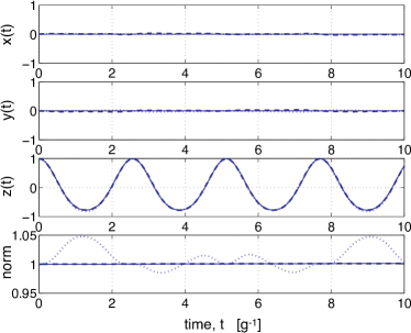
Figure 1: This figure depicts the reduced state calculated by three different methods; the exact solution (solid line), the ensemble average of 1000 SSEs for both the linear (dotted) and actual (dashed) SSE for the coherent unraveling. In this figure all calculations were done using a simple Euler method with a step size of $dt=0.0001$, a detuning of $\Delta=2g$ and initial system state of the form $|{\psi(0)}\rangle=|{e}\rangle$.

V.2 Coherent Unraveling

For the simple system the memory function, Eq. (40) is given by Eq. (142), and and the noise operator for the coherent unraveling is,

$$\hat{z}(t)=g\hat{a}_{1}e^{-i\Delta{t}}+g\hat{a}_{-1}e^{i\Delta{t}}.$$ (154)

The linear SSE was obtained when we assumed an ostensible probability $\Lambda(a_{1},a_{-1})$ equal to the vacuum distribution

$$\Lambda(a_{1},a_{-1})=\pi^{-2}e^{-|a_{1}|^{2}-|a_{-1}|^{2}}.$$ (155)

With this probability distribution, we can write the noise function as a random variable equation of the form,

$${z}(t)=g{a}_{1}e^{-i\Delta{t}}+g{a}_{-1}e^{i\Delta{t}},$$ (156)

where $a_{1}$ and $a_{-1}$ are complex GRVs of mean 0 and variance 1.

Applying the simple systems dynamics to equation (55) we obtain

$$\partial_{t}|{\tilde{\psi}_{z}({t})}\rangle=\Big{(}z^{*}(t)\hat{\sigma}-\hat{\sigma}^{\dagger}\int_{0}^{t}\alpha{(t-s)}\frac{\delta}{\delta z^{*}(s)}ds\Big{)}|{\tilde{\psi}_{z}({t})}\rangle.$$ (157)

In Sec. III.2 we made the general Ansatz described by Eq. (56). For this simple system the specific Ansatz we will use is

$$\frac{\delta}{\delta z^{*}(s)}|{\tilde{\psi}_{z}({t})}\rangle=f(t,s)\hat{\sigma}|{\tilde{\psi}_{z}({t})}\rangle.$$ (158)

To work out the functions $f(t,s)$ we use the following consistency condition DioGisStr98 ,

$$\frac{\delta}{\delta z^{*}(s)}\frac{\partial}{\partial t}|{\tilde{\psi}_{z}({t})}\rangle=\frac{\partial}{\partial t}\frac{\delta}{\delta z^{*}(s)}|{\tilde{\psi}_{z}({t})}\rangle,$$ (159)

This gives

$$\partial_{t}f(t,s)\hat{\sigma}|{\tilde{\psi}_{z}({t})}\rangle=f(t,s)F(t)\hat{\sigma}|{\tilde{\psi}_{z}({t})}\rangle,$$ (160)

where

$$F(t)=\int_{0}^{t}\alpha{(t-s)}f(t,s)ds.$$ (161)

This allows us to write the linear SSE for the coherent unraveling as

$$\partial_{t}|{\tilde{\psi}_{z}({t})}\rangle=\Big{[}z^{*}(t)\hat{\sigma}-\hat{\sigma}^{\dagger}\hat{\sigma}F(t)\Big{]}|{\tilde{\psi}_{z}({t})}\rangle.$$ (162)

This is simple to to solve numerically provide we have a solution for $F(t)$.

The best way to calculate $F(t)$ is to split it into to two terms, $F(t)=F_{1}(t)+F_{-1}(t)$ where,

$$F_{1}(t)=\int_{0}^{t}|g|^{2}e^{-i\Delta(t-s)}f(t,s)ds=F_{-1}^{*}(t).$$ (163)

Differentiating the above equations for $F_{1}(t)$ and $F_{-1}(t)$ and using Eq. (160) and the fact that $f(t,t)=1$ yields

$$d_{t}F_{1}(t) = |g|^{2}-i\Delta F_{1}(t)+F_{1}(t)F(t),$$ (164)

$$d_{t}F_{-1}(t) = |g|^{2}+i\Delta F_{-1}(t)+F_{-1}(t)F(t),$$ (165)

which can be solved numerically. The initial conditions are $F(0)=F_{1}(0)=F_{-1}(0)=0$. Writing $|{\tilde{\psi}_{z}({t})}\rangle=C_{e}(t)|{e}\rangle+C_{b}(t)|{b}\rangle$ gives us the following two differential equations,

$$d_{t}C_{e}(t) = -C_{e}(t)F(t),$$ (166)

$$d_{t}C_{b}(t) = z^{*}(t)C_{e}(t).$$ (167)

For an excited-state initial condition these equation can be solve numerically. Note that these solutions will not remain normalized, and the norm of most of them becomes very small. This reflects the fact that a typical individual solution of this SSE does not correspond to a typical measurement result. Nevertheless, the ensemble average of the unnormalized states is $\rho_{\rm red}(t)$. To show this we simulated 1000 SSE for different $z(t)$. The results of this simulation are shown in Fig. 1 as a dotted line, where the agreement with the exact solution is good.

The actual SSE for coherent unraveling is found by applying the above results to Eq. (III.3). Doing this we obtain

$$\partial_{t}|{\psi_{z}({t})}\rangle = \Big{\{}(\hat{\sigma}-\langle\hat{\sigma}\rangle_{t})z^{*}(t)-(\hat{\sigma}^{\dagger}-\langle\hat{\sigma}^{\dagger}\rangle_{t})\hat{\sigma}F(t)$$ (168)

$$+\Big{\langle}(\hat{\sigma}^{\dagger}-\langle\hat{\sigma}^{\dagger}\rangle_{t})\hat{\sigma}\Big{\rangle}_{t}F(t)\Big{\}}|{\psi_{z}({t})}\rangle.$$

The noise, $z^{*}(t)$ in this equation is given by,

$$z^{*}(t)=z_{\Lambda}^{*}(t)+\int_{0}^{t}\alpha^{*}{(t-s)}\langle\hat{\sigma}^{\dagger}\rangle_{s}ds,$$ (169)

where $z_{\Lambda}(t)$ is the noise function used in the linear case. With this SSE the two differential equations for the complex amplitudes become

$$d_{t}C_{e}(t) = -C_{e}^{2}(t)C_{b}^{*}(t)z^{*}(t)+F(t)C_{e}(t)(-1$$ (170)

$$+|C_{e}(t)|^{2}-|C_{e}(t)|^{2}|C_{b}(t)|^{2}),$$

$$d_{t}C_{b}(t) = C_{e}(t)(1-|C_{b}(t)|^{2})z^{*}(t)+F(t)C_{b}(t)|C_{e}(t)|^{2}$$ (171)

$$\times(2-|C_{b}(t)|^{2}).$$

The solution to these equations is an actual state, in the sense that it is normalized, and generated with the actual probabilities. Thus a typical trajectory does give, at any time $t$, a typical state that corresponds to an observer measuring it at that time in the coherent basis. It is thus worth examining a typical trajectory, which we have plotted in Fig. 2 (the solid line). The normalization of the state is shown to remain equal to one, within the error introduced by the integration algorithm. To show that the ensemble average of these trajectories is the reduced state, an ensemble average of 1000 SSE was simulated and the results are depicted in Fig. 1 (dashed line). We see that the actual case is closer to the $\rho_{\rm red}(t)$ then the linear case. This is expected as in general the linear SSE converges slower than the actual SSE, as most of the states generated from the linear SSE have virtually no contribution to the mean.

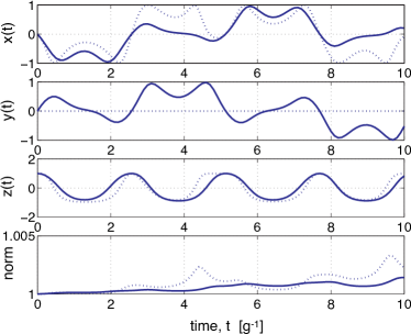
Figure 2: This figure shows a typical trajectory generated by the actual SSE for both the coherent (solid) and quadrature (dotted) unraveling. These were all done with the parameters defined in Fig. 1.

V.3 Quadrature Unraveling

If we apply the theory for the quadrature unraveling to this simple system, the quadrature noise operator, equation (95) becomes

$$\hat{z}(t)=2g\{\hat{X}_{1}^{+}\cos(\Delta{t)})+\hat{Y}_{1}^{-}\sin(\Delta{t})\},$$ (172)

and the quadrature noise function is

$${z}(t)=2g\{{X}_{1}^{+}\cos(\Delta{t})+{Y}_{1}^{-}\sin(\Delta{t})\},$$ (173)

which is real. If we choose the ostensible probability to equal the vacuum probability, then

$$\Lambda(X_{1}^{+},Y_{1}^{-})=\pi^{-1}{e^{-{X_{1}^{+}}^{2}-{Y_{1}^{-}}^{2}}}.$$ (174)

Thus for the linear case ${X}_{1}^{+}$ and ${Y}_{1}^{-}$ are GRVs of mean zero and variance $1/2$.

For this simple system the quadrature linear SSE, Eq. (121), becomes

$$\partial_{t}|{\tilde{\psi}_{z}({t})}\rangle=\Big{(}z(t)\hat{\sigma}-\hat{\sigma}_{x}\int_{0}^{t}\beta{(t-s)}\frac{\delta}{\delta z(s)}ds\Big{)}|{\tilde{\psi}_{z}({t})}\rangle$$ (175)

As for the coherent case we can make an Ansatz for the functional derivative. We again choose Eq. (158). This allows us to write the quadrature linear SSE as

$$\partial_{t}|{\tilde{\psi}_{z}({t})}\rangle=\Big{(}z(t)\hat{\sigma}-\hat{\sigma}_{x}\hat{\sigma}F(t)\Big{)}|{\tilde{\psi}_{z}({t})}\rangle,$$ (176)

where $F(t)$ is given by

$$F(t)=\int_{0}^{t}\beta{(t-s)}f(t,s)ds,$$ (177)

and $\beta{(t-s)}=2|g|^{2}\cos(\Delta(t-s))$.

It turns out for this simple system $F(t)$ is the same for both the coherent and quadrature unraveling, because $\alpha{(t-s)}=\beta{(t-s)}$. Knowing $F(t)$, we get the following two differential equations for the state:

$$d_{t}C_{e}(t) = -C_{e}(t)F(t),$$ (178)

$$d_{t}C_{b}(t) = z(t)C_{e}(t).$$ (179)

These are the same as for the coherent case, except that $z(t)$ is generated differently. To show that the ensemble average of the solution to the linear SSE for the quadrature unraveling converges to $\rho_{\rm red}(t)$, 1000 trajectories for different $z(t)$ where simulated. The results of these simulations are shown in Fig. 3 as a dotted line, where it is seen that the ensemble average of the linear SSE does reproduce the exact solution for $\rho_{\rm red}(t)$ with little error.

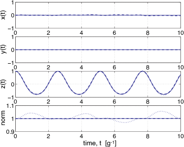
Figure 3: This figure depicts the reduced state calculated by three different methods; the exact solution (solid line), the ensemble average of 1000 SSEs for both the linear (dotted) and actual (dashed) SSE for the quadrature unraveling. These where all done with the parameters defined in Fig. 1.

The actual SSE for quadrature unraveling is found by applying the above results to Eq. (137),

$$\partial_{t}|{\psi_{z}({t})}\rangle = \Big{\{}(\hat{\sigma}-\langle\hat{\sigma}\rangle_{t})z(t)-(\hat{\sigma}_{x}-\langle\hat{\sigma}_{x}\rangle_{t})\hat{\sigma}F(t)$$ (180)

$$+\Big{\langle}(\hat{\sigma}_{x}-\langle\hat{\sigma}_{x}\rangle_{t})\hat{\sigma}\Big{\rangle}_{t}F(t)\Big{\}}|{\psi_{z}({t})}\rangle.$$

The noise, $z(t)$ in this equation is given by,

$$z(t)=z_{\Lambda}(t)+\int_{0}^{t}\beta{(t-s)}\langle\hat{\sigma}_{x}\rangle_{s}ds,$$ (181)

where $z_{\Lambda}(t)$ is the noise function used in the linear case. With this SSE the two differential equations for the complex amplitudes become,

$$d_{t}C_{e}(t) = F(t)C_{e}(t)(-1+|C_{e}(t)|^{2}-|C_{e}(t)|^{2}|C_{b}(t)|^{2})$$ (182)

$$-F(t)C_{e}^{3}(t){C_{b}^{*}}^{2}(t)-C_{e}^{2}(t)C_{b}^{*}(t)z(t),$$

$$d_{t}C_{b}(t) = F(t)C_{b}(t)|C_{e}(t)|^{2}(2-|C_{b}(t)|^{2})$$ (183)

$$+F(t)C_{b}^{*}(t)C_{e}^{2}(t)(1-|C_{b}(t)|^{2})+C_{e}(t)$$

$$\times(1-|C_{b}(t)|^{2})z(t).$$

A typical trajectory from the quadrature SSE is illustrated in Fig. 2 (the dotted line). Note the feature that clearly distinguishes it from the coherent trajectory: $y$ is always zero. To show that the solution of the actual SSE reproduces the reduced state on average, an ensemble of 1000 actual SSEs was simulated and the results are depicted in Fig. 3 (dashed line). We see that it reproduces the exact solution, again with less error than that from the linear SSE.

VI Discussion and Conclusions

In this paper we have explored non-Markovian stochastic Schrödinger equations by furthering the work of Diosi, Strunz and Gisin Str96 ; Dio96 ; DioStr97 ; DioGisStr98 ; StrDioGis99 . Specifically, we have interpreted their results in the framework of quantum measurement theory. Their SSEs arise as a special case when the measurement basis of the bath is the coherent states, so we label it the coherent unraveling. The benefit of using the measurement interpretation is two-fold.

First, it allows us a better understanding of the interpretation of non-Markovian SSEs. The state at any time $t$ generated by the SSE can be interpreted as a conditioned system state, given a particular result from a particular measurement on the bath. However, the measurements at different times are incompatible, so the linking together of different states over time is, we have argued, a convenient fiction. Thus the trajectory generated by a non-Markovian SSE does not have the same physical status as that generated by a Markovian SSE, where the measurements at different times are compatible and the states at different times can represent a single evolving system.

Second, it allows us to generate other sorts of SSEs corresponding to different sorts of measurements on the bath (unravelings). In this paper we presented a second unraveling, based on measuring certain quadrature operators on the bath. This gives rise to an SSE only under certain assumptions to do with the bath frequencies and couplings. The resultant SSE contains real-valued noise, as opposed to the complex noise in the SSE of DSG. The ability to construct a non-Markovian SSE with real-valued noise is contrary to the expectation expressed by DSG in DioGisStr98 .

We have also shown in this paper that the Markov limit of the quadrature and coherent unravelings are homodyne and heterodyne detection respectively. As noted above, in this Markov limit the SSE generates a true quantum trajectory for a conditioned system state over time. It is interesting that this arises smoothly as the limit of a non-Markovian SSE that does not have this interpretation. However, as we have shown, one has to be very careful with the definition of the time of measurement in order to reconcile this limit with the usual quantum trajectory theory.

To illustrate our general theory we have applied it to a simple system: a TLA coupled linearly to just two single-mode fields detuned from the atom by $\pm\Delta$. This is an extremely non-Markovian problem with no finite memory time, unlike the previous examples considered by DSG. Nevertheless the theory is able to describe the evolution of the atom by an SSE. In Fig. 2 we displayed typical non-Markovian SSEs for both the quadrature and coherent unraveling, and in Figs. 1 and 3 we showed that on average both SSEs do generate the exact reduced state.

In conclusion this paper has presented a significant generalization of the DSG approach to non-Markovian SSE. However, there is still a lot of questions to be answered.

First, is it possible within this framework to derive other classes of non-Markovian SSEs? In particular, is it possible to describe an unraveling based on discrete measurement on the bath, say the in number-state basis?

Second, is there a physical system where our theory could be naturally applied? That is, is there a physical system where the bath could be measured in a suitable basis at an arbitrary time so as to produce a pure conditioned system state?

Third, what conditions are necessary for one to be able to find a suitable Ansatz for replacing the functional derivative with an operator? As we have argued, this is necessary to create a genuine SSE. Yu, Diósi, Gisin and Strunz have given a general procedure for finding this operator, but only when the system dynamics are weakly non-Markovian (the so-called ‘post-Markovian’ approximation) YuDioGisStr99 ; YuDioGisStr00 . We suspect that the conditions for finding an exact Ansatz depend upon both the nature of the system and its coupling to the bath.

Fourth, can the techniques of non-Markovian SSEs be applied as a numerical tool for studying real systems? We have in mind potentially strongly non-Markovian systems such as an atom laser Hop or photon emission in a photonic band-gap material Joh84 ; BayLamMol97 .

Fifth, and last, is there an alternative framework to standard quantum measurement theory in which there is a physical interpretation for a trajectory generated by a non-Markovian SSE? That is, can the states at different times in a single trajectory generated by the SSE be interpreted as pertaining to a single system in some non-standard approach to quantum measurements? This is a very open question.

References

- (1) H.J. Carmichael, An Open Systems Approach to Quantum Optics (Springer-Verlag, Berlin, 1993).
- (2) C.W. Gardiner, Quantum Noise (Springer-Verlag, Berlin, 1991).
- (3) W.H. Lindblad, Commun. Math. Phys. 48, 199, (1976).
- (4) L. Diósi, Phys. Lett. A 132, 233, (1988).
- (5) L. Diósi, J. Phys. A 21, 2885, (1988).
- (6) V.P. Belavkin, “Nondemolition measurement and nonlinear filtering of quantum stochastic processes”, pp. 245-66 of A. Blaquière (ed.), Lecture Notes in Control and Information Sciences 121 (Springer, Berlin, 1988).
- (7) V.P. Belavkin and P. Staszewski, Phys. Rev. A 45, 1347, (1992).
- (8) A. Barchielli, Quantum Opt. 2, 423, (1990).
- (9) A. Barchielli, Int. J. Theor. Phys 32, 2221, (1993).
- (10) N. Gisin and I.C. Percival, Phys. Lett. A 167, 315 (1992).
- (11) N. Gisin and I.C. Percival, J. Phys. A 25, 5677, (1992).
- (12) N. Gisin and I.C. Percival, J. Phys. A: Math. Gen. 26, 2233, (1993).
- (13) J. Dalibard, Y. Castin and K. Mølmer, Phys. Rev. Lett. 68, 580, (1992).
- (14) C.W. Gardiner, A.S. Parkins and P. Zoller, Phys. Rev. A 46, 4363, (1992).
- (15) A. Imamoglu, Phys. Rev. A 50, 3650, (1994).
- (16) W.T. Strunz, Phys. Lett. A 224, 25, (1996).
- (17) M.W. Jack and M.J. Collett, Phys. Rev. A 61, 062106, (2000).
- (18) J.D. Cresser, Laser Phys. 10, 1, (2000).
- (19) L. Diósi, Quantum Semiclass. Opt. 8, 309, (1996).
- (20) L. Diósi and W.T. Strunz, Phys. Lett. A 2358, 569, (1997).
- (21) L. Diósi, N. Gisin and W.T. Strunz, Phys. Rev. A 58, 1699, (1998).
- (22) W.T. Strunz, L. Diósi and N. Gisin, Phys. Rev. Lett. 82, 1801, (1999).
- (23) W.T. Strunz, L. Diósi, N. Gisin and T. Yu, Phys. Rev. Lett. 83, 4909 , (1999).
- (24) H.M. Wiseman and G.J. Milburn, Phys. Rev. A 47, 642, (1993).
- (25) H.M. Wiseman and G.J. Milburn, Phys. Rev. A 47, 1652, (1993).
- (26) H.M. Wiseman, Quantum Semiclass. Opt. 8, 205, (1996).
- (27) M.W. Jack, M.J. Collett and D.F. Walls, Phys. Rev. A 59, 2306, (1999).
- (28) J. Gambetta and H.M. Wiseman, Phys. Rev. A 64, 042105, (2001).
- (29) P. Warszawski, H. M. Wiseman and H. Mabuchi, Phys. Rev. A 65, 023802, (2001).
- (30) V.B. Braginsky and F. Y. Khalili, Quantum Measurement (Cambridge University Press, Cambridge, 1992).
- (31) K. Kraus, States, Effects, and Operations: Fundamental Notions of Quantum Theory (Springer, Berlin, 1983).
- (32) M.O. Scully and M.S. Zubairy, Quantum Optics (Cambridge University Press, Cambridge, 1997).
- (33) P. Goetsch and R. Graham, Phys. Rev. A 50, 5242, (1994).
- (34) D. Gatarek and N. Gisin, J. Math. Phys. 32, 2152, (1991).
- (35) C.W. Gardiner, Handbook of Stochastic Methods: for Physics, Chemistry and the Natural Science (Springer-Verlag, Berlin, 1983).
- (36) F.E. van Dorsselaer and G. Nienhuis, J. Opt. B: Quantum Semiclass. Opt. 2, R25, (2000).
- (37) R.G. Parr and W. Yang, Density-Functional Theory of Atoms and Molecules (Oxford University Press, New York, 1989).
- (38) C. W. Gardiner and M. J. Collett, Phys. Rev. A 31, 3761 (1985).
- (39) T. Yu, L. Diósi, N. Gisin and W.T. Strunz, Phys. Rev. A 60, 91, (1999).
- (40) T. Yu, L. Diósi, N. Gisin and W.T. Strunz, Phys. lett. A 265, 331, (2000).
- (41) J.J. Hope, G.M. Moy, M.J. Collett and C.M. Savage, Phys. Rev. A 61, 023603, (2000).
- (42) S. John, Phys. Rev. Lett. 53 2169, (1984).
- (43) S. Bay, P. Lambropoulos, and K. Mølmer, Phys. Rev. Lett. 79 2654, (1997).