Comparison of Star and Ring Topologies for Entanglement Distribution

Abstract

We investigate the differences between distributing entanglement using star and ring type network topologies. Assuming symmetrically distributed users, we asses the relative merits of the two network topologies as a function of the number of users when the amount of resources and the type of the quantum channel are kept fixed. For limited resources, we find that the topology better suited for entanglement distribution could differ from that which is more suitable for classical communications.

I Introduction

In quantum information processing, entanglement revs is a particularly useful resource and has many applications such as secret key distribution Ek , teleportation ben and dense coding wies . Recently, these quantum communication protocols have been implemented impl . It is imaginable that in the future a large number of distant users would want to engage in communicating with each other through quantum protocols. To enable this to happen, such distant users will need to share particles in maximally entangled states, irrespective of noise in the entanglement distribution channels. Various schemes have been put forward which could directly or indirectly help in such distribution of entanglement qdistr1 ; purf1 ; purf2 ; purf21 ; bhm ; zuk ; multswp ; seriesswp ; qreapt , and have been experimentally demonstrated distrexpts . Given a certain physical distribution of users intending to communicate quantum mechanically, one can connect them with quantum channels to construct networks for the distribution of entanglement. Networks for such entanglement distribution can have different architectures depending on which users are linked directly by quantum channels and which users are indirectly linked through intermediate nodes.

In classical networks, two of the major network topologies are the star network and the ring network. In a ring network, one continuous ring joins all parties who wish to communicate (as shown in Fig.1(a)), whereas in a star network all parties are connected to a central hub where information is exchanged (as shown in Fig.1(b)). If all the nodes of such classical networks are assumed to be free from attacks and failures, then wire length becomes the variable of interest for comparison of the two network types - i.e., one network is said to be better than the other when it requires less wire to construct. This is because noise in the connecting channels is unimportant for classical communications. No matter how noisy the connecting channels are, classical information can be amplified arbitrarily and sent faultlessly through these channels. Based on the wire-length criterion, for networks having the simple circular layouts with symmetrically placed users, as shown in Fig.1, the ring network is better than a star network when the number of users is $N\geq 6$, while the reverse holds true for $N<6$.

For a quantum network, however, we use entanglement, rather than wire-length, as a figure of merit in comparing networks. This is due to the fact that when distributing entanglement via quantum channels, unavoidable noise always degrades perfect entanglement in the transmission process and consequently it is not as easy to reliably distribute entanglement. We therefore use the criterion that the better network is the one that permits the sharing of a greater amount of entanglement between pairs of users on average.

To begin, we tackle the problem for a general channel, when the available resources are unlimited or so large that asymptotic entanglement distillation protocols purf1 ; purf2 ; purf21 can be used as a part of the entanglement distribution method. Note that physically such a situation is permitted only when each user can ”store” qubits noiselessly for a long time. This gives them the chance to manipulate a large number of qubits together, as is required for asymptotic entanglement distillation. In this asymptotic case, we find the criterion for better entanglement distribution becomes equivalent to the wire-length criterion of classical networks. Next we examine two cases of extremely limited resources (only one initial entangled pair available to one user, and exactly one initial entangled pair available to each user) with a specific quantum channel to illustrate the fact that the network for better entanglement distribution can differ sharply from that for better classical communications. After that, we give a heuristic explanation of this striking difference between the cases of limited and infinite resources as seen in our specific examples.

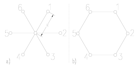
Figure 1: This figure illustrates the two types of network topologies considered, in this case for 6 parties. Each party is located at a corner of regular hexagon. The small circles denote a party and connecting lines denote connecting quantum channels through which entanglement is distributed. R denotes the distance of parties from the center.

II A General Formulation of the Problem

We consider a very simple type of network to facilitate study of the problem. Suppose there are $N$ parties, who are distributed in a circle at a constant distance R from the centre, and wish to share entanglement. They connect themselves using quantum channels using either a star or a ring layout (see Fig.1). As the number $N$ increases, the distance between a party and its neighbors decreases. We define a ’wirelength’ as the shortest connection available on either network - for the ring network this is the channel between neighbors and for the star network it is the channel between one party and the hub.

When any two parties wish to share entanglement, they must use some distribution method to share entanglement between themselves using the most efficient route available to them for the network they are connected by. For a given channel, this method will involve sharing entangled pairs either directly between the two interested parties or between intermediate parties and then joining them using entanglement swapping zuk ; multswp ; seriesswp ; qreapt . There may be some form of distillation involved to concentrate the intermediate or final entanglement in the distribution. In general, one will have to adopt a specific entanglement distillation protocol. It could be asymptotic or non-asymptotic, depending on the availability of resources. It may be optimal or non-optimal depending on whether the knowledge of the optimal distillation protocol exists for the classes states generated during distribution through the channels provided, and whether technology exists for its implementation. A specific type of quantum channel and associated entanglement distillation protocol (not necessarily optimal), together with entanglement swapping to link up adjacent nodes, will comprise a specific distribution method. The basic approach of this paper will be to first choose a specific distribution method and then compare its efficiency on the star and the ring lay-outs. The variables which describe the quantum channel available between two parties are:

• $n$ - the number of wirelengths between them

• $d$ - the length of the wirelengths between them

To clarify this, consider Fig. 1 which shows 6 parties of whom two may wish to communicate. If parties 1 and 4 wish to share entanglement, then using the star network (Fig. 1(a)) they must use $n=2$ wirelengths of length $d=R$ each. If they are connected using the ring network (Fig. 1(b)) then they must use $n=3$ wirelengths of length $d=2R\sin(\frac{\pi}{6})$ each.

Let us define a function $E(d,n)$ which gives the entanglement distributed between two parties separated by $n$ wirelengths each of length $d$. To be able to compare the two network layouts we calculate an $E_{av}$ which is the distributed entanglement averaged over all possible pairs of parties who wish to communicate:

$$E_{av}=\frac{1}{N-1}\sum\limits_{n=1}^{N-1}E(d,n)$$ (1)

For a star network $d$ is always $R$ and $n$ is always $2$ so we have:

$$E_{av}^{star}=E(R,2)$$ (2)

For a ring network, $d$ is the distance between two neighboring parties, and is $2R\sin(\frac{\pi}{N})$ so we have:

$$E_{av}^{ring}=\frac{1}{N-1}\sum\limits_{n=1}^{N-1}E\left(2R\sin\left(\frac{\pi}{N}\right),n\right)$$ (3)

Bearing in mind that in a ring network entanglement can be distributed either way round the network means this formula can be refined to always use the shortest distance:

$$E_{av}^{ring}=\frac{1}{N-1}2\sum\limits_{n=1}^{U}E\left(2R\sin\left(\frac{\pi}{N}\right),n\right)+\mu E\left(2R\sin\left(\frac{\pi}{N}\right),N/2\right)$$ (4)

where $U=(N-1)/2$ if $N$ is odd or $N/2-1$ if N is even and $\mu$ is 0 if $N$ is odd, or 1 if $N$ is even.

To find at what point one layout becomes better than the other, we are interested in finding, for a particular distribution method, the $n$ where:

$$E_{av}^{ring}=E_{av}^{star}$$ (5)

We are interested in comparing how this value of $N$ compares with the classical case, where, for parameters we specify, the ring network became better than the star network as the number of parties is increased. For a classical network, as noted before, this occurs at $N=6$.

Unfortunately there is no analytic formula available for the function $E(d,n)$ for an arbitrary quantum channel. This is because $E(d,n)$ represents the amount of entanglement that can be distilled from a state after decoherence during transmission through a noisy channel. No general formula is known yet for the distillable entanglement of a given state. Despite this fact, it is possible (as we will show) to provide a general statement about the case when an unlimited number of pairs are available across each wirelength. However, when only a limited amount of resources are available per user, we have to rely on the explicit form of the distillable entanglement. In case of limited resources, we will therefore calculate $E(d,n)$ for specific circumstances (specific channel types and specific distribution methods) and use in Eq.(1). The cases we consider are:

• Distributing an unlimited number of pairs along each wirelength and linking each wirelength up using entanglement swapping. We consider a general noisy channel for this case.

• Distributing one pair traveling from source to destination along one or more wirelengths. We use a specific type of quantum channel and a specific distribution method.

• Distributing one pair between each party, and then using entanglement swapping to link them up. We use a specific type of channel for this case as well.

We then try to investigate and explain the trends observed in the above specific cases.

III The case of an unlimited number of pairs for a general channel

First we consider the case where the parties in the network share a very large number $T$ of maximally entangled pairs. An equal number $T/N$ is given to each party. In the case of a ring network each party then sends one half of the pair to their neighbour on the left whereas in a star network each party would send one half to a central hub. The consequence is that in either case, $T/N$ pairs are shared across each wirelength. Since $T$ was very large, $T/N$ is very large (assuming $N$ stays small, of course) and so an asymptotic number of maximally entangled pairs can be distilled across each wirelength i.e. $(T/N)E_{D}$ where $E_{D}$ is the distillable entanglement of a pair that has decohered on travel through the wirelength. In this asymptotic case we assume that the maximally entangled states can be collected together in each wirelength and then matched (i.e., aligned end to end) with maximally entangled states in adjacent wirelengths. The ability to do this would depend on being able to discriminate and store the distilled maximally entangled states. Connecting up adjacent maximally entangled pairs in succession by entanglement swapping then produces $(T/N)E_{D}$ maximally entangled pairs shared between any two users. In this asymptotic case, the same entanglement arises independent of the number of wirelengths separating two users. In Eq.(1) then $E$ becomes a function of only the length $d$ of a single wirelength. Therefore because $E$ depends only on $d$, the situation becomes equivalent to the classical case and the crossover at which the ring network becomes better than the star network is also at $N=6$. This is because for $N=6$ a radial wirelength has the same length as a circumferential wirelength and therefore $E_{D}$ will be the same for states travsersing the star or ring networks. For $N<6$ the radial wirelengths are shorter than circumferential ones and so $E_{D}$ will be greater for states passing through a star network. For $N>6$ then circumferential wirelengths are shorter and so the ring network gives a greater overall entanglement.

IV One Pair Travelling All The Way For A Bit-Flip Channel

In this scenario we suppose that only one entangled pair is provided to any one of the users and he may have to communicate with any of the other users through a bit-flip channel. This means that the two parties must distribute the single pair between themselves. In the case of a star network one party sends one half of the pair to a central point and then on again to the other party. For a ring network the half of the pair would travel around the ring through other parties until it reached the destination party. This channel acts on states in the following way:

$$\left|\psi^{+}\right\rangle\left\langle\psi^{+}\right|\rightarrow\Lambda=\lambda\left|\psi^{+}\right\rangle\left\langle\psi^{+}\right|+(1-\lambda)\left|\phi^{+}\right\rangle\left\langle\phi^{+}\right|$$ (6)

We relate $\lambda$ to the length of the channel $d$ by:

$$\lambda=\frac{1+e^{-d}}{2}$$ (7)

For such states the maximum distillable entanglement is known vp to be $1-S(\Lambda)$ where $S(\Lambda)$ denotes the Von Neumann entropy of the state $\Lambda$.

One particle was kept at the originator while the other was sent to the other party, passing through one or more wirelength to reach it. Fig.2 shows $E_{av}^{ring}$ and $E_{av}^{star}$ plotted against $N$. We see that right from the start ($N=2$) the ring layout is better. This is true for all values of the radius $R$ of the network. So we see a difference from the classical case where it was only at $N=6$ that the ring network became better than the star network.

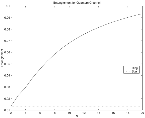
Figure 2: This figure plots the average entanglement for a ring network (solid line) and a star network (dotted line) against the number of users in the network when only one entangled pair is available to travel the entire distance between parties intending to communicate. This graph is true for all values of the radius $R$ and the channel type is bit-flip.

V One Pair Between Each Party For A Bit-Flip Channel

In this scenario we consider each party in the network having one maximally entangled pair. Each party then sends one particle of the pair to their neighbour through a bitflip channel. Entanglement swapping is then used to create a link between any two parties who wish to share entanglement. The procedure of entanglement swapping produces a pair linking across the two original pairs with a fidelity given by:

$$F_{n}=1+2F_{a}F_{b}-F_{a}-F_{b}$$ (8)

Figure 3: This figure plots the average entanglement for a ring network (solid line) and a star network (dotted line) against the number of users in the network when only one entangled pair is available in each wirelength. This graph is true for all values of the radius $R$ and the channel type is bit-flip.

For a bit-flip channel, the order in which pairs are connected by entanglement swapping does not matter. Fig.3 shows $E_{av}^{ring}$ and $E_{av}^{star}$ plotted against $N$. We see again that straight away the ring layout is better. In fact, due to the nature of the bit-flip channel, the resultant fidelities for this situation and the previous one where one pair is shared across the entire distance between the two communicating parties, turn out to be identical.

Thus in the case dealt with in sections IV and V, it becomes apparent that the results of comparing network topologies for entanglement distribution can be very different from the classical case.

VI A Heuristic Explanation Of The Results

In this section, we attempt to explain heuristically the difference in the results for the unlimited number of pairs (where the ring network becomes better than the star network only after there are more than $6$ parties in the network), and the result for one pair (where the ring network is always better than the star network).

We will first give a general description which encompasses both the case for an unlimited number of pairs and that for a small number of pairs between parties. When a distillation procedure operates on a finite ensemble finite , we generally have outcomes of various degrees of entanglement with various probabilities. In these outcomes, the entanglement is either pumped up or pumped down from the original values. To try to express a general pattern, we restrict ourselves to distribution methods obeying the following assumptions:

1. Assume a general distillation protocol operating on arbitrarily sized ensembles (finite or infinite) where there is a probability $p$ that distillation in a wirelength is successful and boosts the entanglement to $E_{D}+\delta_{s}$, $E_{D}$ being the distillable entanglement of the state. There is a probability $1-p$ that it fails and the entanglement is reduced to $E_{D}-\delta_{f}$. In most cases there will be more than two possible outcomes of a general distillation protocol, but for simplicity we assume just two outcomes.

2. Assume $E_{D}+\delta_{s}$ is quite near to maximal so that the entanglement swapping to connect adjacent wirelengths is near perfect. When adjacent pairs are connected using entanglement swapping we assume that the resultant entanglement is equal to the lower value of the two pairs. Therefore when connecting $n$ wirelengths, the entanglement will be the lowest value of the $n$ wirelengths.

Using these rules, we can formulate the following expression for the average entanglement obtained over $n$ wirelengths:

$$p^{n}(E_{D}+\delta_{s})+(1-p^{n})(E_{D}-\delta_{f})=E_{D}+p^{n}(\delta_{s}+\delta_{f})-\delta_{f}.$$ (9)

As we move from distributing a finite number of entangled pairs to an infinite number the $\delta$’s will tend to zero and $p\rightarrow 1$, meaning the average entanglement will asymptotically tend to approach the distillable entanglement. To make it more clear, in the asymptotic case we have a unit probability ($p\rightarrow 1$) conversion of a homogenous ensemble to an inhomogenous ensemble of maximally entangled and unentangled pairs with the fraction of maximally entangled pairs being $E_{D}$. This fraction $E_{D}$ of maximally entangled pairs in each wirelength can now be connected with unit efficiency using entanglement swapping. Asymptotic distillation essentially conserves the distillable entanglement and tiny fluctuations $\delta$ in the final entanglement tend to zero. If we put $p\rightarrow 1$ and $\delta\rightarrow 0$ in Eq.(9) we are left with with an average of $E_{D}$ over different lengths and the merit of the star and the ring networks simply depends on the total wirelength. In the other extreme (non asymptotic), the fluctuation $\delta$ is large (say of the order $~{}E_{D}$) and we compare $\sum_{n}p^{n}$ with $p^{2}$. This leads to the behaviour of ring always being better than the star. Thus we have successfully interpolated between the case of distributing a finite number of entangled pairs to an infinite number.

Note that in the above presentation, asymptotic distillation has been viewed in a rather different angle than usual. Usually $E_{D}$ is interpreted as the probability of a successful distillation and the entanglement produced as a result of a successful distillation is maximal. We invert the interpretation of this same process as a method succeeding with probability $p=1$ and creating an amount of entanglement $E_{D}$ per initial impure pair in the form of maximally entangled pairs. In this latter (maximally entangled) form, the pairs can be connected in series without any loss of entanglement through entanglement swapping.

In order to illustrate the meaning of the above heuristic approach with specific values of $p$ and $\delta$’s we consider an example - a watched amplitude damped channel where we distribute the state $\frac{1}{\sqrt{2}}\left(\left|00\right\rangle+\left|11\right\rangle\right)$, with two pairs between connected users to obtain a case somewhat intermediate between the previous examples.

$$\begin{array}[]{lll}|\Psi^{{}^{\prime}}\rangle_{12E_{1}E_{2}}&=&\frac{1}{\sqrt{2}}(\sqrt{1+e^{-4d}}[\frac{\left|00\right\rangle+e^{-2d}\left|11\right\rangle}{\sqrt{1+e^{-4d}}}]_{12}\left|00\right\rangle_{E_{1}E_{2}}\\ &+&e^{-d}\sqrt{1-e^{-2d}}\left|01\right\rangle_{12}\left|10\right\rangle_{E_{1}E_{2}}\par\\ &+&e^{-d}\sqrt{1-e^{-2d}}\left|10\right\rangle_{12}\left|01\right\rangle_{E_{1}E_{2}}\\ &+&(1-e^{-2d})\left|00\right\rangle_{12}\left|11\right\rangle_{E_{1}E_{2}})\end{array}$$ (10)

Then, if the environment is being monitored, there is a probability of $\frac{1}{2}\left(1+e^{-4d}\right)$ that the state observed is (corresponds to the state $\left|00\right\rangle_{E_{1}E_{2}}$ of the environment)

$$|\Psi^{{}^{\prime}}_{c}\rangle_{12}=\frac{1}{\sqrt{1+e^{-4d}}}\left(\left|00\right\rangle+e^{-2d}\left|11\right\rangle\right)$$ (11)

where the subscript $c$ represents the fact that this state is a result of conditional evolution. $|\Psi^{{}^{\prime}}_{c}\rangle_{12}$ is not maximally entangled and must now be purified. One method of doing this is to use the Procrustean method. This has probability of producing a maximally entangled stated (MES) of twice the modulus squared of the lower coefficient. i.e.

$$\frac{2e^{-4d}}{1+e^{-4d}}$$ (12)

We combine the probability of observation with that of purification to give an expression for $p$ i.e. the successful concentration to an MES.

$$p=e^{-4d}$$ (13)

Before the entanglement was $E_{D}$, now it is 1. So

$$\delta_{s}=1-E_{D}$$ (14)

$$\delta_{f}=E_{D}$$ (15)

So the expression for the average entanglement above becomes:

$$e^{-4nd}$$ (16)

With this expression for one pair having been distributed, the ring network is immediately better than the star network as before.

VII Conclusions

In this paper, we have compared entanglement distribution between several users connected by star and ring network configurations. We have shown that the cross over point at which the ring network becomes better than the star network varies with the amount of resources. When the amount of resources is limited and cannot be stored, so that the number of entangled pairs available across a channel at a time is finite, then the results for entanglement distribution can differ sharply from that for classical communications. We have given a heuristic explanation of this fact that it stems from the comparison of different powers of probabilities arising in the comparison of star and ring networks. However, in the asymptotic case (which can physically arise when we can store particles for long and can process a large number of shared entangled pairs parallelly) the relative merits of the star and the ring configurations are the same as classical.

We have arrived at our conclusions by considering extreme examples. At one extreme is just one pair per wirelength and just one pair available to travel all the way from user to user. At the other extreme is a very large number of pairs shared in parallel between each adjacent user (or user and node) in which asymptotic manipulations of entanglement are used. As we gradually increase the number of pairs available to be processed parallelly between users from $1$ to $\infty$, we would expect the cross over point in $N$ to increase from $1$ to $6$. This is because when more and more pairs can be stored, we have a greater chance of selectively connecting the higher entangled pairs in adjacent wirelengths. When the number of pairs becomes really large, this selective connection becomes really successful and gives just the entanglement in a single wirelength as the effective criterion for comparison. In the future, we intend to investigate explicit examples when an intermediate number of pairs are shared in parallel per wirelength to explore the transition from the non-asymptotic to the asymptotic case.

VIII Acknowledgements

AH thanks the UK EPSRC (Engineering and Physical Sciences Research Council) for financial support.

References

- (1) M.B. Plenio and V. Vedral, Cont. Phys. 39, 431 (1998); A. Zeilinger, Phys. World 11, 35 (1998).
- (2) A. K. Ekert, Phys. Rev. Lett. 67, 661 (1991).
- (3) C. H. Bennett, G. Brassard, C. Crepeau, R. Jozsa, A. Peres and W. K. Wootters, Phys. Rev. Lett. 70, 1895 (1993).
- (4) C. H. Bennett and S. J. Wiesner, Phys. Rev. Lett. 69, 2881 (1992).
- (5) K. Mattle, H. Weinfurter, P. G. Kwiat and A. Zeilinger, Phys. Rev. Lett. 76, 4656 (1996); D. Bouwmeester, J-W. Pan, K. Mattle, M. Eibl, H. Weinfurter, and A. Zeilinger, Nature (London) 390, 575 (1997); D. Boschi, S. Branca, F. De Martini, L. Hardy and S. Popescu, Phys. Rev. Lett. 80, 1121 (1998); A. Furasawa, J.L.Sørensen, S.L. Braunstein, C.A.Fuchs, H.J.Kimble and E.S.Polzik, Science 282, 706 (1998); W. Tittel, J. Brendel, H. Zbinden and N. Gisin, Phys. Rev. Lett. 84, 4737 (2000); T. Jennewein, C. Simon, G. Weihs, H. Weinfurter and A. Zeilinger, Phys. Rev. Lett. 84, 4729 (2000).
- (6) J. I. Cirac, A. K. Ekert, S. F. Huelga and C. Macchiavello, Phys. Rev. A 59, 4249 (1999).
- (7) C. H. Bennett, H. J. Bernstein, S. Popescu and B. Schumacher, Phys. Rev. A 53, 2046 (1996); N. Gisin, Phys. Lett. A 210, 151 (1996).
- (8) C. H. Bennett, D. P. DiVincenzo, J. A. Smolin and W. K. Wootters, Phys. Rev. A 54, 3824 (1996).
- (9) C. H. Bennett, G. Brassard, S. Popescu, B. Schumacher, J. A. Smolin and W. K. Wootters, Phys. Rev. Lett. 76, 722 (1996); D. Deutsch, A. Ekert, R. Jozsa, C. Macchiavello, S. Popescu and A. Sanpera, Phys. Rev. Lett. 77, 2818 (1996).
- (10) E. Biham, B. Huttner and T. Mor, Phys. Rev. A 54, 2651 (1996).
- (11) M. Zukowski, A. Zeilinger, M. Horne and A. K. Ekert, Phys. Rev. Lett. 71, 4287 (1993).
- (12) S. Bose, V. Vedral and P. L. Knight, Phys. Rev. A 57, 822 (1998).
- (13) S. Bose, V. Vedral and P. L. Knight, Phys. Rev. A 60, 194 (1999); L. Hardy and D. D. Song, Phys. Rev. A 62, 052315 (2000); B.-S. Shi, Y.-K. Jiang and G.-C. Guo, Phys. Rev. A 62, 054301 (2000); M. Cinchetti and J. Twamley, Phys. Rev. A 63, 052310 (2001).
- (14) H.-J. Briegel, W. Dür, J. I. Cirac and P. Zoller, Phys. Rev. Lett. 81 5932 (1998); W. Dür, H.-J. Briegel, J. I. Cirac and P. Zoller, Phys. Rev. A 59, 169 (1999).
- (15) J.-W. Pan, D. Bouwmeester, H. Weinfurter, and A. Zeilinger, Phys. Rev. Lett. 80, 3891 (1998); P. G. Kwiat, S. Barraza-Lopez, A. Stefanov and N. Gisin, Nature 409, 1014 (2001); J.-W. Pan, C. Simon, C. Brukner and A. Zeilinger, Nature 410, 1067 (2001).
- (16) V. Vedral and M. B. Plenio, Phys. Rev. A 57, 1619 (1998).
- (17) H.-K. Lo and S. Popescu, Phys. Rev. A 63, 022301 (2001); M. A. Nielsen, Phys. Rev. Lett. 83, 436 (1999); G. Vidal, Phys. Rev. Lett. 83, 1046 (1999); D. Jonathan and M. B. Plenio, Phys. Rev. Lett. 83, 1455 (1999); L. Hardy, Phys. Rev. A 60, 1912 (1999); D. Jonathan and M. B. Plenio, Phys. Rev. Lett. 83, 3566 (1999).