Spin squeezing via quantum feedback

Abstract

We propose a quantum feedback scheme for producing deterministically reproducible spin squeezing. The results of a continuous nondemolition atom number measurement are fed back to control the quantum state of the sample. For large samples and strong cavity coupling, the squeezing parameter minimum scales inversely with atom number, approaching the Heisenberg limit. Furthermore, ceasing the measurement and feedback when this minimum has been reached will leave the sample in the maximally squeezed spin state.

Squeezed spin systems KitUed93 of atoms and ions have attracted considerable attention in recent years due to the potential for practical applications, such as in the fields of quantum information QInf98 and high-precision spectroscopy Spect . Quantum correlations of squeezed spin states outperform classical states in analogy with squeezed optical fields. Moreover, squeezed spin sates are also multiparticle entangled states Soretal01 . Recent proposals for their generation include the absorption of squeezed light sqzlight , collisional interactions in Bose-Einstein condensates Soretal01 ; collBEC , and direct coupling to an entangled state through intermediate states such as collective motional modes for ions MolSor99 or molecular states for atoms HelmYou01 .

Other proposals create spin squeezing via quantum nondemolition (QND) measurements KuzBigMan98 ; KuzManBig00 ; Duanetal00 . A striking recent achievement of QND measurements is the entanglement of two macroscopic atomic samples JulKozPol01 . These QND schemes produce conditional squeezed states that are dependent on the measurement record. On the other hand, unconditional squeezing would ensure that the state is deterministically reproducible. Mølmer Mol99 has shown that alternating QND measurements and incoherent feedback can produce sub-Poissonian number correlations. However, that work does not treat the quantum effects of the measurement back action or the feedback on the mean spin (which is assumed to be zero). Hence it cannot predict the strength of the entanglement.

In this Rapid Communication, we suggest achieving spin squeezing via feedback that is coherent and continuous. We consider a continuous QND measurement of the total population difference of an atomic sample. The results of the measurement, which conditionally squeeze the atomic sample, are used to drive the system into the desired, deterministic, squeezed spin state. This involves amplitude modulation of a radio-frequency (rf) magnetic field, where the feedback strength varies in time such that the mean number difference is kept at zero.

An ensemble of $N$ two-level atoms can be described by a spin-$J$ system Dic54 , i.e., a collection of $2J=N$ spin-$\frac{1}{2}$ particles. The collective spin operators are given by $J_{\alpha}=\sum_{k=1}^{N}\mbox{$\frac{1}{2}$}\sigma^{(k)}_{\alpha}(\alpha=x,y,z)$, where $\sigma_{\alpha}^{(k)}$ are the Pauli operators for each particle. Thus, $J_{z}$ represents half the total population difference. Coherent spin states (CSS) have variances normal to the mean spin direction equal to the standard quantum limit (SQL) of $J/2$. Introducing quantum correlations among the atoms reduces the variance below the SQL in one direction at the expense of the other KitUed93 . Such squeezed spin states can be characterized by the squeezing parameter Soretal01

$$\xi^{2}_{{\mathbf{n}}_{1}}=N(\Delta J_{{\mathbf{n}}_{1}})^{2}/(\left\langle{J_{{\mathbf{n}}_{2}}}\right\rangle^{2}+\left\langle{J_{{\mathbf{n}}_{3}}}\right\rangle^{2}),$$ (1)

where ${\mathbf{n}}_{i}(i=1,2,3)$ are orthogonal unit vectors. Systems with $\xi^{2}_{\mathbf{n}}<1$ are spin squeezed in the direction ${\mathbf{n}}$ and also have multiparticle entanglement Soretal01 .

Let the internal states, $|{1}\rangle$ and $|{2}\rangle$, of each atom be the degenerate magnetic sublevels of a $J=\mbox{$\frac{1}{2}$}$ state, e.g., an alkali ground state. Each atom is prepared in an equal superposition of the two internal states, thus giving a CSS of length $J$ in the $x$-direction. The atomic sample is placed in a strongly driven, heavily damped, optical cavity, as shown in Fig. 1$(a)$. The cavity field is assumed to be far off resonance with respect to transitions probing state $|{2}\rangle$, see Fig. 1$(b)$. This dispersive interaction causes a phase shift of the cavity field proportional to the number of atoms in $|{2}\rangle$. Thus, the QND measurement of $J_{z}$ (since $N$ is conserved) is effected by the homodyne detection of the light exiting the cavity CorMil98 .

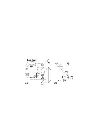
Figure 1: $(a)$ Schematic experimental configuration. A cavity field of amplitude $i|\beta|$ interacts with the atomic sample. The current $I_{c}(t)$ from the homodyne detection of the cavity output, damped at rate $\kappa$, is combined with $\lambda(t)$ produced by a signal generator (SG). The combined signal controls the amplitude (AM) of an rf magnetic field that, together with a static field, drives $J_{y}$. $(b)$ Single atom diagram. The static B field lifts the degeneracy of the magnetic sublevels. The far-detuned cavity field $i|\beta|$ monitors the collective population in state $|{2}\rangle$ (and hence $J_{z}$). The rf driving field, applied perpendicularly to the static field direction, induces magnetic dipole transitions between $|{1}\rangle$ and $|{2}\rangle$ (thus driving $J_{y}$).

This interaction is defined by the Hamiltonian $\hbar\chi J_{z}b^{\dagger}b$ where $b$,$b^{\dagger}$ are the cavity field operators and $\chi=g^{2}/4\Delta$, with one-photon Rabi frequency $g$, and optical detuning $\Delta$ CorMil98 . For strong coherent driving we can use the semiclassical approximation $b\to i|\beta|+b$, where now $b$ represents small quantum fluctuations around the classical amplitude $i|\beta|$. The interaction is thus

$$H_{\rm int}=\hbar\chi|\beta|J_{z}(-ib+ib^{\dagger}),$$ (2)

where we have chosen an initial $J_{z}$ splitting of $-\chi|\beta|^{2}$.

Following the procedure of Sec. VII in Ref. WisMil94 we can adiabatically eliminate the cavity dynamics if the cavity decay rate $\kappa\gg\chi|\beta|J_{z}$, which requires $\kappa\gg\chi|\beta|\sqrt{N}$ (since the initial $\Delta J_{z}=\sqrt{J/2}$). The evolution of the atomic system due the measurement is thus

$$\dot{\rho}=M{\cal D}[J_{z}]\rho,$$ (3)

where $M=4\chi^{2}|\beta|^{2}/\kappa$ is the measurement strength [equivalent to $2D$ in Eq. (22) of Ref. CorMil98 ], and ${\cal D}[r]\rho\equiv r\rho r^{\dagger}-(r^{\dagger}r\rho+\rho r^{\dagger}r)/2$. This equation represents decoherence of the atomic system due to photon number fluctuations in the cavity field, with the result of increased noise in the spin components normal to $J_{z}$.

The effect of Eq. (2) on the cavity field is a phase shift proportional to $J_{z}$, and thus the output Homodyne photocurrent is given by WisMil94

$$I_{c}(t)=2\sqrt{M}\left\langle{J_{z}}\right\rangle_{c}+\zeta(t),$$ (4)

where $\zeta(t)$ is a white-noise term satisfying ${\rm E}[\zeta(t)\zeta(t^{\prime})]=\delta(t-t^{\prime})$ and ${\rm E}$ is the ensemble average. The conditional master equation for the atomic system is then WisMil94

$$d\rho_{c}=dtM{\cal D}[J_{z}]\rho_{c}+\sqrt{M}dW(t){\cal H}[J_{z}]\rho_{c},$$ (5)

where $dW(t)=\zeta(t)dt$ is an infinitesimal Wiener increment and ${\cal H}[r]\rho\equiv r\rho+\rho r^{\dagger}-{\rm Tr}[(r+r^{\dagger})\rho]\rho$.

The effects of this evolution on the initial CSS are a decrease in the variance of $J_{z}$ with corresponding increases for $J_{y}$ and $J_{x}$ (i.e., spin squeezing), as well as a stochastic shift of the mean $J_{z}$ away from its initial value of zero. This shift, indicated by state 2 of Fig. 2, is equal to

$$d\left\langle{J_{z}}\right\rangle_{c}=2\sqrt{M}dW(t)(\Delta J_{z})^{2}_{c}\\ \approx 2\sqrt{M}I_{c}(t)dt\left\langle{J_{z}^{2}}\right\rangle_{c}.$$

Here the approximation assumes that $\left\langle{J_{z}}\right\rangle_{c}=0$, which will be relevant when feedback is in place.

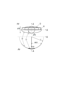
Figure 2: Schematic $(a)$ $y-z$ and $(b)$ $x-y$ projections of the quasiprobability distributions for the spin state. The spin states are represented by ellipses on a sphere of radius $J$. The initial CSS, spin polarized in the $x$ direction, is given by state 1. State 2 is one particular conditioned spin state after a measurement of $J_{z}$, while state 3 is the corresponding ensemble average state. The effect of the feedback is shown by state 4. A rotation about the $y$ axis shifts the conditioned state 2 back to $\left\langle{J_{z}}\right\rangle_{c}=0$. The ensemble average of these conditioned states will then be similar to state 4.

The average or unconditioned evolution, Eq. (3), is simply recovered by taking the ensemble average of all possible conditioned states, i.e., $\rho(t)={\rm E}[\rho_{c}(t)]$. This leads to a spin state with $J_{z}$ variance equal to $J/2$. In other words, the unmonitored measurement does not affect $J_{z}$ and the squeezed character of the individual conditioned states is lost, indicated by state 3 in Fig. 2.

To retain the reduced fluctuations of $J_{z}$ in the average evolution, we employ a feedback mechanism that uses the measurement record to continuously drive the system into the $\left\langle{J_{z}}\right\rangle_{c}=0$ squeezed state. The idea is to cancel the stochastic shift of $\left\langle{J_{z}}\right\rangle_{c}$ due to the measurement. This simply requires a rotation of the mean spin about the $y$ axis equal and opposite to that caused by Eq. (Spin squeezing via quantum feedback), as illustrated in Fig. 2. The feedback Hamiltonian must therefore take the form

$$H_{\rm fb}(t)=\lambda(t)I_{c}(t)J_{y}/\sqrt{M},$$ (6)

where $\lambda(t)$ is a time-varying feedback strength. This feedback driving can be implemented by modulating an applied rf magnetic field Sangetal01 , as shown in Fig. 1.

Following again the methods of Ref. WisMil94 to find the total stochastic master equation, we can calculate the conditioned shift of the mean $J_{z}$ due to the feedback. Again using the assumption that $\left\langle{J_{z}}\right\rangle_{c}=0$ we have

$$d\left\langle{J_{z}}\right\rangle_{\rm fb}\approx-\lambda(t)I_{c}(t)dt\left\langle{J_{x}}\right\rangle_{c}/\sqrt{M}.$$ (7)

Since the idea is to produce $\left\langle{J_{z}}\right\rangle_{c}=0$ via the feedback, the approximations above and in Eq. (Spin squeezing via quantum feedback) apply and we find that the required feedback strength is

$$\lambda(t)=2M\left\langle{J_{z}^{2}}\right\rangle_{c}/\left\langle{J_{x}}\right\rangle_{c}.$$ (8)

This type of feedback control is essentially a form of state-estimation-based feedback Dohetal00 . Although Eq. (6) looks like direct current feedback, the strength of this feedback (8) is determined by conditioned state expectation values. $I_{c}(t)$ only appears directly in $H_{\rm fb}$ due to the assumption that the feedback works and so $\left\langle{J_{z}}\right\rangle_{c}=0$.

Being dependent on conditioned expectation values, which are computationally very expensive, Eq. (8) is not practical in an experimental sense. What is required is a predetermined series of data points or ideally an equation for $\lambda(t)$, like in Fig. 1. To find a suitable expression we begin by assuming the feedback is successful and replace the conditioned averages by ensemble averages,

$$\lambda(t)\simeq 2M\left\langle{J_{z}^{2}}\right\rangle/\left\langle{J_{x}}\right\rangle.$$ (9)

This approximation will be valid if the unconditioned state has high purity since then it must comprise of nearly identical highly pure conditioned states.

The evaluation of both the purity (${\rm Tr}[\rho^{2}]$) and the averages in Eq. (9) ($\left\langle{A}\right\rangle\equiv{\rm Tr}[A\rho]$) requires the unconditioned master equation (ME) WisMil94

$$\dot{\rho}=M{\cal D}[J_{z}]\rho-i\lambda(t)[J_{y},J_{z}\rho+\rho J_{z}]+\frac{\lambda(t)^{2}}{M}{\cal D}[J_{y}]\rho.$$ (10)

The terms in this equation describe, respectively, the noise due to the measurement back-action, the feedback optical driving, and the noise introduced by the feedback. The state determined by Eq. (10), with $\lambda(t)$ given by Eq. (9), has a purity very close to one (see below). Since the state is very close to a pure state, we are justified in applying the approximation of Eq. (9).

Note that Eq. (10) describes the exact unconditioned evolution of the atomic system where the feedback strength is arbitrarily defined by $\lambda(t)$. Equation (9) thus describes one particular feedback scheme, however, it can only (easily) be evaluated numerically. To find an approximate analytical expression we look at when $\left\langle{\mathbf{J}}\right\rangle\sim{\cal O}(J)$, for which the atomic sample remains near the minimum uncertainty state $\left\langle{J_{y}^{2}}\right\rangle\left\langle{J_{z}^{2}}\right\rangle\approx J^{2}/4$. This is equivalent to a linear approximation represented by replacing $J_{x}$ with $J$ in the commutator $[J_{y},J_{z}]=iJ_{x}$, which allows us to calculate $\left\langle{J_{y}^{2}}\right\rangle$ directly from the ME (and hence $\left\langle{J_{z}^{2}}\right\rangle$). The decrease of $\left\langle{J_{x}}\right\rangle$ from $J$ is then related to the increase of $\left\langle{J_{y}^{2}}\right\rangle$ from $J/2$ [see Fig. 2$(b)$] due to the measurement back action. Using these approximations we obtain

$$\lambda(t)\approx Me^{Mt/2}(1+2JMt)^{-1}.$$ (11)

We can analytically approximate the degree of squeezing produced by the particular feedback scheme represented by Eq. (11). For our model Eq. (1) becomes

$$\xi^{2}_{z}=\frac{N\left\langle{J_{z}^{2}}\right\rangle}{\left\langle{J_{x}}\right\rangle^{2}}\simeq\frac{\lambda(t)J}{M\left\langle{J_{x}}\right\rangle}\approx e^{Mt}(1+2JMt)^{-1}.$$ (12)

This leads to a minimum at $t_{*}\approx 1/M$ of

$$\xi^{2}_{\rm min}\approx e/2J,~{}~{}J\gg 1.$$ (13)

Thus, the minimum attainable squeezing parameter asymptotically approaches an inverse dependence on the sample size, i.e., the Heisenberg limit AndLuk01 .

The approximations leading up to Eqs. (9) and (11) can be justified by numerically solving the ME (10) for a given $\lambda(t)$, for example, using the Matlab quantum optics toolbox Tan99 . The approximation of Eq. (9) can be tested by calculating the purity for $\rho$ described by the ME with this particular feedback. The expectation values in $\lambda(t)$ are found by iteratively solving the ME [updating $\lambda(t)$ each time step], and thus we also have

$$\xi^{2}_{z}=2J\left\langle{J_{z}^{2}}\right\rangle/\left\langle{J_{x}}\right\rangle^{2}.$$ (14)

The results of this simulation are shown in Fig. 3$(a)$, where the purity is given by the dotted curve and $\xi^{2}_{z}$ is curve A. Clearly, the purity remains near unity for times of interest. This implies that the measurement and feedback scheme has worked to produce nearly identical, nearly pure, conditioned states [for times ${\cal O}(M^{-1})$], and we are therefore justified in using Eq. (9).

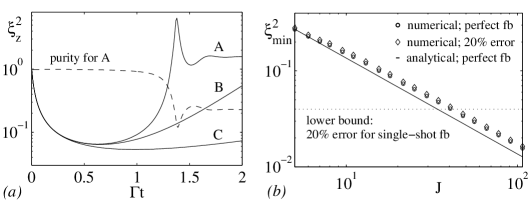
Figure 3: $(a)$ Time dependence of the purity $={\rm Tr}[\rho^{2}]$ (dashed curve), and the squeezing parameter $\xi^{2}_{z}$ (curves A, B, and C). The purity and curve A are the results for a feedback scheme defined by Eq. (9). For comparison, Eq. (14) is also simulated for the scheme defined by Eq. (11) and the result is curve B. Finally, curve C is the approximate analytical expression for squeezing parameter given by Eq. (12). In all cases $J=25$. $(b)$ $J$ dependence of the squeezing parameter minimum, $\xi^{2}_{\rm min}$. Plotted are the results of numerical solutions of the ME, and hence Eq. (14), with $\lambda(t)$ given by Eq. (11) (circles) and $\lambda(t)\times 120\%$ (diamonds). These values approach $1.665/J$ and $1.744/J$, respectively. The dotted line is the lower bound for single-shot feedback also with a $20\%$ error, while the analytical result for perfect continuous feedback, Eq. (13), is the solid line.

The further approximations to obtain the analytical Eq. (11) are also good, as shown by curve B in Fig. 3$(a)$, where the fit to curve A for the early evolution and minimum is nearly perfect. We are not interested in later times since the idea is to cease the measurement and feedback when the minimum $\xi^{2}_{z}$ is reached. The analytical expression for the squeezing parameter, Eq. (12), is also plotted as curve C in Fig. 3$(a)$. Although the minimum is not a perfect fit to the exact numerical results, it has the correct order of magnitude and so we expect the $J^{-1}$ scaling of Eq. (13) to be correct.

The scaling of $\xi^{2}_{\rm min}$ is obtained numerically from solutions of the ME [and thus Eq. (14)] with feedback described by Eq. (11). This $\lambda(t)$, shown above to be a good approximation, is the suitable form for experimental realization. The numerical results, along with the analytical expression (13), are plotted in Fig. 3$(b)$ which clearly verifies the $J^{-1}$ dependence. The analytical coefficient ($e/2$) represents an error of $\sim 18\%$ compared to the numerical fit, and the optimum time ($t_{*}$) is also slightly out as shown by Fig. 3$(a)$. Nevertheless, these errors only apply to scaling coefficients, not to the scalings themselves.

Experimentally, the limit to squeezing will be dominated by spontaneous losses due to absorption of QND probe light. The rate of this loss is $N\gamma\Omega^{2}/4\Delta^{2}$, where $\gamma$ is the spontaneous emission rate and $\Omega=g|\beta|$. To reach the Heisenberg limit (requiring a time $t_{*}=1/M$) we want the total loss to be negligible, i.e., we require

$$N\gamma\frac{\chi|\beta|^{2}}{\Delta}\frac{\kappa}{4\chi^{2}|\beta|^{2}}\sim 1~{}~{}\Rightarrow~{}~{}g^{2}\sim N\kappa\gamma,$$ (15)

which is the very strong coupling regime of cavity QED. Note we also required $\kappa\gg\chi|\beta|\sqrt{N}$ for the adiabatic elimination of the cavity field, and to satisfy both we thus require $\Delta\gg\gamma N^{3/2}$. It is not surprising that Eq. (15) is the same requirement as for André and Lukin’s model AndLuk01 implementing the countertwisting Hamiltonian KitUed93 , since writing Eq. (10) in Lindblad form reveals such a term. Similarly, the condition for achieving some squeezing, i.e., $\xi^{2}<1$, will be $g^{2}N>\kappa\gamma$. Further, we have calculated that a free space model [also given by Eq. (10) but with $M$ equal to $N$ in Ref. WisTho01 ] will also produce some squeezing, although the Heisenberg limit cannot be reached since by $t_{*}=1/M$ all atoms will be lost from the sample.

Figure 3$(b)$ also indicates that our continuous scheme is very robust to any experimental errors in the feedback strength, as opposed to a single-shot method. The latter approach consists of a single (integrated) measurement pulse (see e.g., Ref. Duanetal00 ), followed by a single feedback pulse. If there is a relative error of $\epsilon$ in the feedback strength, this will induce an error term $(\Delta J_{z}^{\rm err})^{2}\sim\epsilon^{2}J/2$, which will dominate the total variance for $J\gg 1$. Thus $\xi^{2}_{\rm min}$ will have a lower bound of $\epsilon^{2}$, and will never be better than $J^{-1}$. On the other hand, as shown in Fig. 3$(b)$, a large ($20\%$) error in $\lambda(t)$ for continuous feedback does not affect the $J^{-1}$ scaling. We have also found this theoretical scaling to be unaffected by inefficient measurements. Finite feedback delay time will also have a limited effect as long as it is faster than $(JM)^{-1}$.

This Rapid Communication has presented a scheme for producing a spin squeezed atomic sample via QND measurement and feedback. The advantage over previous QND schemes KuzBigMan98 ; KuzManBig00 is that it provides unconditional, or deterministically reproducible, squeezing. For very strong cavity coupling, the theoretical squeezing approaches the Heisenberg limit $\xi^{2}\sim 1/N$, while some squeezing will be produced at weaker coupling and even in free space (thus presenting a simple experimental test for quantum feedback). This indicates a stronger squeezing mechanism than collisional interactions in a Bose-Einstein condensate where the scaling is $N^{-2/3}$ Soretal01 ; collBEC . Furthermore, by ceasing the measurement when this minimum is reached, the maximally squeezed state could be maintained indefinitely.

L.K.T and H.M.W wish to acknowledge inspiring discussions with Klaus Mølmer and Eugene Polzik.

References

- (1)
- (2) M. Kitagawa and M. Ueda, Phys. Rev. A 47, 5138 (1993).
- (3) Phys. World 11, 33 (1998), special issue on Quantum Information.
- (4) D. Wineland et al., Phys. Rev. A 50, 67 (1994); P. Bouyer and M. Kasevich, ibid. 56, R1083 (1997).
- (5) A. Sørensen et al., Nature (London) 409, 63 (2001).
- (6) A. Kuzmich, K. Mølmer, and E. S. Polzik, Phys. Rev. Lett. 79, 4782 (1997); A. E. Kozhekin, K. Mølmer, and E. Polzik, Phys. Rev. A 62, 033809 (2000).
- (7) C. K. Law, H. T. Ng, and P. T. Leung, Phys. Rev. A 63, 055601 (2000); U. V. Poulsen and K. Mølmer, ibid. 64, 013616 (2001).
- (8) K. Mølmer and A. Sørensen, Phys. Rev. Lett. 82, 1835 (1999).
- (9) K. Helmerson and L. You, Phys. Rev. Lett. 87, 170402 (2001).
- (10) A. Kuzmich, N. P. Bigelow, and L. Mandel, Europhys. Lett. 42, 481 (1998).
- (11) A. Kuzmich, L. Mandel, and N. P. Bigelow, Phys. Rev. Lett. 85, 1594 (2000).
- (12) L.-M. Duan et al., Phys. Rev. Lett. 85 5643 (2000).
- (13) B. Julsgaard, A. Kozhekin, and E. S. Polzik, Nature (London) 413, 400 (2001).
- (14) K. Mølmer, Eur. Phys. J. D 5, 301 (1999).
- (15) R. H. Dicke, Phys. Rev. 93, 99 (1954).
- (16) J. F. Corney and G. J. Milburn, Phys. Rev. A 58, 2399 (1998).
- (17) H. M. Wiseman and G. J. Milburn, Phys. Rev. A 49, 1350 (1994).
- (18) R. T. Sang et al., Phys. Rev. A 63, 023408 (2001).
- (19) A. C. Doherty et al., Phys. Rev. A 62, 012105 (2000).
- (20) A. André and M. D. Lukin, e-print quant-ph/0112126 (2001).
- (21) S. M. Tan, J. Opt. B: Quantum Semiclassical Opt. 1, 424 (1999).
- (22) H. M. Wiseman and L. K. Thomsen, Phys. Rev. Lett. 86, 1143 (2001).