Atom-laser coherence and its control via feedback

Abstract

We present a quantum-mechanical treatment of the coherence properties of a single-mode atom laser. Specifically, we focus on the quantum phase noise of the atomic field as expressed by the first-order coherence function, for which we derive analytical expressions in various regimes. The decay of this function is characterized by the coherence time, or its reciprocal, the linewidth. A crucial contributor to the linewidth is the collisional interaction of the atoms. We find four distinct regimes for the linewidth with increasing interaction strength. These range from the standard laser linewidth, through quadratic and linear regimes, to another constant regime due to quantum revivals of the coherence function. The laser output is only coherent (Bose degenerate) up to the linear regime. However, we show that application of a quantum nondemolition measurement and feedback scheme will increase, by many orders of magnitude, the range of interaction strengths for which it remains coherent.

I Introduction

The invention of the laser in the late 1950s SchTow58 created the field of quantum optics and continues to lead to an enormous range of scientific and technological applications. It is expected that the realization of “atom lasers” will similarly revolutionize the field of atom optics alaserpot . Atom optics is the study of atoms where their wavelike nature becomes important, suggesting an analogy with photons AdaSigMly94 . An atom laser is therefore defined as a device that produces a continuous beam of intense, highly directional, and coherent matter waves Wis97 , in analogy with the light produced by an optical laser fn-continuous . The ideal atom laser beam is a single frequency (i.e., monochromatic) de Broglie wave with well-defined intensity and phase.

The first experimental achievements of the Bose-Einstein condensation (BEC) of gaseous atoms BECexpt was followed immediately by several independent ideas for creating an atom laser proposals . Since then there have been experimental advances in the coherent release of pulses pulses and quasicontinuous beams beams of atoms from BECs, as well as further theoretical proposals props2 . In the experimental configurations to date, the laser mode is the ground state of a trapped BEC, which is pumped by evaporative cooling of uncondensed atoms, and the out-coupling (separated in time from the pumping) is achieved by either Raman or radio-frequency (rf) transitions to an untrapped state. Although these experimental accomplishments do not include simultaneous pumping and output coupling, they do represent major steps towards achieving an operating atom laser.

Recent experimental KohHanEss01 ; Detetal01 ; LeCoqetal01 and theoretical Wis97 ; Doddetal97 ; ZobMey98 ; GolZobMey98 ; JacNarColWal99 ; HopMoyColSav00 ; RobSavOst01 studies have focused on the fundamental coherence properties of BECs and atom lasers. Atoms (unlike photons) interact with each other, producing strong nonlinearities that affect the coherence of the trapped condensate and thus also the out-coupled laser field. For a single-mode condensate the dominant effect of atomic collisions is to turn number fluctuations into fluctuations in the energy and hence fluctuations in the frequency, thus causing increased phase uncertainty. Collisional interactions therefore lead to a significant decrease in the atom-laser coherence time, and a corresponding increase in the linewidth, especially in the case of BECs formed by evaporative cooling. However, we have previously shown that a continuous, quantum nondemolition (QND) feedback scheme can effectively cancel the linewidth broadening due to such collisions WisTho01 .

To study the coherence properties of an atom laser one can either focus on classical or quantum noise in the atomic field. Sources of classical noise may be technical, such as fluctuations in the trapping potential, finite temperatures, and specific trap geometries Detetal01 , or dynamical, such as three-body recombination RobSavOst01 . The study of these effects is usually based on mean-field laser models described by Gross-Pitaevskii (GP)-type equations LanLifPit80 . Quantum noise is an intrinsic part of the atomic system as a consequence of the uncertainty relations and is the limiting contribution to coherence. The study of this requires a fully quantum-mechanical approach, of which the most common is based on the quantum optical master equation WalMil94 . The complexities of either approach, which individually require approximations to facilitate theoretical analysis, indicate that simultaneous analysis would not be easy fn-hope .

In this paper we present a fully quantum mechanical treatment of the coherence of a single-mode atom laser and its control via the QND feedback scheme proposed in Ref. WisTho01 . Specifically, we study the properties of the first-order coherence function (i.e. phase coherence), which allows us to derive the coherence time (and hence laser linewidth) as well as the power spectrum of the laser output. Section II summarizes a set of requirements for the coherence of an atom laser first detailed in Ref. Wis97 . Section III presents our mathematical model for the atom laser and shows the resulting linewidth for increasing atomic interaction strength. Numerical methods are presented in Sec. III B, while the analytical results are discussed in Sec. III C. When the collisional nonlinearity is very strong, the coherence function undergoes a quantum collapse and revival sequence (detailed in III D). This leads to an interesting regime in the power spectrum (detailed in III E), which has not been considered before. Section IV details the effects of feedback based on a physically reasonable QND measurement of the condensate number, to include all regimes of the nonlinearity. Section V concludes.

II Requirements for coherence

The coherence of an atom-laser beam can be defined analogously to that of an optical laser beam Wis97 . The fundamental assumption is that the laser output is well approximated by a highly directional classical wave of fixed intensity and phase, which is also ideally restricted to a single transverse mode. The output should also be a stationary process, i.e., its statistics should be independent of time. To be coherent, the laser output should then additionally have $(1)$ a relatively small spread of longitudinal spatial frequencies (i.e. be monochromatic); $(2)$ a relatively stable intensity (i.e. be approximately second-order coherent); and $(3)$ a relatively stable phase (i.e. have a relatively slow decay of first-order coherence).

The first condition, monochromaticity, follows from the requirement that the laser output approximates a classical wave. It can, therefore, be expressed in terms of the characteristic coherence length of the wave, $l_{\rm coh}=(\delta k)^{-1}$, i.e. the reciprocal of the spatial frequency spread. Condition (I) becomes

$$l_{\rm coh}\gg\bar{\lambda}=2\pi/\bar{k},$$ (1)

i.e., that the coherence length be much greater than the mean atomic wavelength Wis97 . In terms of the spectral width or linewidth, $\ell\equiv\delta\omega$, the monochromaticity requirement simply becomes $\ell\ll\bar{\omega}$, where the mean frequency $\bar{\omega}$ is defined by the kinetic energy of the atoms, i.e., $\bar{\omega}=\hbar\bar{k}^{2}/2m$. Condition (I) also guarantees that the dispersion of an atomic beam will be negligible over the coherence length Wis97 .

To explain the second and third conditions we require a many-body description of the output beam; see Ref. Wis97 for an in-depth discussion. Basically, the output field of a laser can be represented by the localized field annihilation operator $b(t)$, which approximately satisfies the $\delta$-function commutation relation

$$[b(t),b^{\dagger}(t^{\prime})]=\delta(t-t^{\prime}),$$ (2)

at a given point in the output. Thus, $I(t)=b^{\dagger}(t)b(t)$ can be interpreted as the approximate atom-flux operator. The fundamental assumption of a laser is that the output should be well approximated by a classical wave of fixed intensity and phase. This is therefore represented mathematically by

$$b(t)\approx\beta(t)\equiv\beta e^{-i\bar{\omega}t},$$ (3)

where $\beta$ is a complex number and the trivial time dependence emphasizes that the laser output should be stationary. The atomic field is not exactly a classical wave because there are fluctuations in the field amplitude due to classical and quantum sources of noise. These will need to be small or somehow cancelled to maximize coherence.

It can be argued that there are no mean fields in both atom and quantum optics Mol97 , and as such the description of a laser as a coherent state is a “convenient fiction”. Despite this, mean-field theories (e.g., based on GP equations) are very successful in describing the properties of lasers, as is the use of initial coherent states for solving and visualizing master equations (as done in this paper). A vanishing mean field means that

$$\left\langle{b(t)}\right\rangle=0.$$ (4)

In the case of optical lasers the output might, in principle, be in a state with well-defined amplitude and phase. But since we do not know the absolute phase, an average over all possible phases gives Eq. (4). For atom lasers, only bilinear combinations of the atom field are observable and similarly no Hamiltonian is linear in the atom field (atoms cannot be created out of nothing). Thus a mean field amplitude is physically impossible and the absolute phase is unobservable, again giving Eq. (4).

Since the mean field of a laser is zero, we cannot require $\left\langle{b(t)}\right\rangle=\beta$. However, for approximating $b(t)$ by $\beta(t)$, we can require that the mean intensity be given by

$$\left\langle{I(t)}\right\rangle=\left\langle{b^{\dagger}(t)b(t)}\right\rangle=|\beta|^{2},$$ (5)

and also that the fluctuations in intensity should be small in some sense. This requirement is quantified using Glauber’s normalized second-order coherence function (for a stationary system) Glau63 :

$$g^{(2)}(\tau)=\left\langle{:I(t+\tau)I(t):}\right\rangle/\left\langle{I(t)}\right\rangle^{2},$$ (6)

where the $\left\langle{:\ :}\right\rangle$ denotes normal ordering.

For a field that is second-order coherent, i.e. $g^{(2)}(\tau)=1$, there is no correlation between the arrival times of bosons at a detector and their distribution is Poissonian. Specifically the probability for detecting a boson in the interval $(t+\tau,t+\tau+dt)$ given one detected at time $t$ is $g^{(2)}(\tau)\left\langle{I(t)}\right\rangle dt$. For the intensity fluctuations to be small we therefore require that Wis97

$$|g^{(2)}(\tau)-1|\ll 1,$$ (7)

i.e. the laser output should be approximately second-order coherent: condition (II).

Assuming that condition (II) is met, the intensity of the laser beam will be relatively stable and the only significant variation in the output field will be due to phase fluctuations. A useful measure of the phase fluctuations is the stationary first-order coherence function Glau63 :

$$G^{(1)}(\tau)=\left\langle{b^{\dagger}(t+\tau)b(t)}\right\rangle,$$ (8)

or its normalized form:

$$g^{(1)}(\tau)=G^{(1)}(\tau)/\left\langle{b^{\dagger}(t)b(t)}\right\rangle.$$ (9)

Unlike the field $b(t)$ itself, the bilinear combinations above are measurable even for an atom field. $G^{(1)}(\tau)$ is simply the mean intensity (5) when $\tau=0$ and as $\tau$ increases, it decreases towards zero as the phase becomes decorrelated from its initial value at $t$.

So, the phase of the field might be undefined because it varies in time, i.e., the first-order coherence decays. Although we cannot expect the laser to be approximately first-order coherent for all time [i.e., $g^{(1)}(\tau)\approx 1$], we can require the decay of $g^{(1)}(\tau)$ to be slow in some sense. The characteristic time for this decay is simply the coherence time, which can be defined as Wis97

$$\tau_{\rm coh}=\frac{1}{2}\int_{0}^{\infty}|g^{(1)}(\tau)|d\tau.$$ (10)

This is the time over which the phase of the field is relatively constant.

But even if the phase is constant, it might also be undefined due to a large intrinsic quantum uncertainty given by $\Delta\phi\Delta n\geq 1/2$ Hol84 . Since typically $\Delta n\leq\bar{n}$, the quantum phase uncertainty will be large if the mean number $\bar{n}$ is small. For the phase to be well defined we therefore need the field to have a large intensity, i.e., $\bar{n}\gg 1$, over the time that the phase of the field is constant, i.e., for times $T\ll\tau_{\rm coh}$. The number of bosons in the output field for a given duration $T$ is $\bar{n}=\left\langle{I(t)}\right\rangle T$. Thus, for a well-defined phase we require $\left\langle{I(t)}\right\rangle\tau_{\rm coh}\gg 1$. In terms of the first-order coherence function this translates to Wis97

$$\left\langle{I(t)}\right\rangle\int|g^{(1)}(\tau)|d\tau=\int|G^{(1)}(\tau)|d\tau\gg 1,$$ (11)

which quantifies the requirement that the decay of first-order coherence be relatively slow: condition (III).

This condition for coherence is equivalent to the requirement that the output field be highly Bose-degenerate Wis97 , which is rarely considered for optical lasers because it is so easily satisfied. It requires that the output atom flux, i.e., $\left\langle{I(t)}\right\rangle$, be much larger than the linewidth $\delta\omega$. Since the atom-laser linewidth is the reciprocal of the coherence time, i.e.,

$$\ell\equiv\delta\omega=1/\tau_{\rm coh},$$ (12)

we find that condition (I) requires $\ell\ll\bar{\omega}$ and condition (III) requires

$$\ell\ll\left\langle{I(t)}\right\rangle.$$ (13)

For single-mode optical lasers typically $\left\langle{I(t)}\right\rangle>\bar{\omega}$ so condition (III) is always satisfied. On the other hand, the collisional interactions in atom lasers causes significant linewidth broadening and so satisfying (III) is not guaranteed. However, in Sec. IV we show that this broadening can be effectively cancelled by a QND measurement and feedback scheme.

The linewidth, or spectral width, of a field is usually defined as the full width at half-maximum height (FWHM) of the output power spectrum. In general, the power spectrum is given by the Fourier transform of the first-order coherence function WalMil94 :

$$P(\omega)=\int_{-\infty}^{\infty}G^{(1)}(\tau)e^{-i\omega\tau}d\tau.$$ (14)

This is defined so that $\int_{-\infty}^{\infty}P(\omega)d\omega=\left\langle{I(t)}\right\rangle$ and therefore can be interpreted as the steady-state flux per unit frequency fn-pspec .

If the first-order coherence function has the form $G^{(1)}(\tau)\propto\exp(-\gamma\tau)$ then the laser output will have a Lorentzian power spectrum. In this case the FWMH is exactly equal to the linewidth as defined in Eq. (12), i.e. the reciprocal of the coherence time. On the other hand, if $G^{(1)}(\tau)\propto\exp(-\gamma^{2}\tau^{2})$ then the laser has a Gaussian power spectrum with a FWHM that is now only approximately equal to the linewidth.

In any case, if the first-order coherence function has the form $G^{(1)}(\tau)=|G^{(1)}(\tau)|\exp(i\bar{\omega}\tau)$, then condition (III) for coherence can be restated in terms of the maximum spectral intensity $P(\bar{\omega})$. From Eqs. (14) and (10) and the above assumption (Appendix A shows that this is a good approximation for the atom laser), we find

$$P(\bar{\omega})=\int_{-\infty}^{\infty}|G^{(1)}(\tau)|d\tau=4\left\langle{I(t)}\right\rangle\tau_{\rm coh}.$$ (15)

Thus, regardless of the resultant shape of the output power spectrum, condition (III) becomes

$$P(\bar{\omega})\gg 1.$$ (16)

Note that the central frequency $\bar{\omega}$ will be shifted by any laser dynamics which cause a rotation of the mean phase of the laser field.

The remaining sections of this paper present a study of the quantum phase dynamics of the atom laser and thus the coherence properties of its output. Specifically we study the first-order coherence function as a measure of phase fluctuations, which (in the absence of intensity fluctuations) will be the limiting factor to the coherence time of an atom laser. This function, as indicated in this section, is also intrinsically related to the laser output characteristics of linewidth and power spectrum.

III Atom-laser linewidth

III.1 Atom-laser dynamics

The atom-laser model consists of a source of atoms irreversibly coupled to a laser mode, which is supported in a trap that allows an output beam to form. A broadband reservoir acting both as a pump and a sink is also coupled to the source modes. The laser mode and source can be modelled by the ground and excited states of a trapped boson field, representing the condensed and uncondensed atoms, respectively Wis97 . Gain can be achieved, for example, by evaporative cooling of the uncondensed atoms. Out-coupling from the laser mode can be accomplished, for example, by coherently driving condensed atoms into an untrapped electronic state. This model can be simply described by a quantum optical master equation for the laser mode alone Wis97 ; Wis99 , obtained by adiabatically eliminating the source modes and tracing over the continuum of output modes. The system is thus characterized by a wavefunction $\Phi({\bf r})$ and annihilation operator $a$ for the condensate mode.

Far above threshold, the laser mode has Poissonian number statistics Lou73 ; SarScuLam74 . In the absence of thermal or other excess noise, its dynamics are modelled by the completely positive master equation Wis97 ; Wis99

$$\dot{\rho}=\kappa\mu{\cal D}[a^{\dagger}]{\cal A}[a^{\dagger}]^{-1}\rho+\kappa{\cal D}[a]\rho\equiv{\cal L}_{0}\rho,$$ (17)

where the superoperators ${\cal D}$ and ${\cal A}$ are defined as usual for an arbitrary operator $r$:

$${\cal D}[r]\rho\equiv r\rho r^{\dagger}-{\cal A}[r]\rho,~{}~{}{\cal A}[r]\rho\equiv\mbox{$\frac{1}{2}$}\{r^{\dagger}r,\rho\}.$$ (18)

That the master equation is of the Lindblad form follows from the identity

$${\cal D}[a^{\dagger}]{\cal A}[a^{\dagger}]^{-1}=\int_{0}^{\infty}dq{\cal D}[a^{\dagger}e^{-qaa^{\dagger}/2}].$$ (19)

The first term of Eq. (17) represents linear output coupling at rate $\kappa$ and the second term represents nonlinear (saturated) pumping far above threshold, where $\mu\gg 1$ is the stationary mean boson number. It is the decreasing difference between the gain and loss, as the laser is pumped above threshold, that gives rise to the gain-narrowed laser linewidth WalMil94 . The localized output mode operator $b$ of the preceding section is then related to the laser mode via $b=\nu+\sqrt{\kappa}a$, where $\nu$ represents vacuum fluctuations GarQnoise . Note also that we have chosen a reference potential energy for the system such that there is no Hamiltonian $\propto a^{\dagger}a$ in the master equation.

To include the effects of atom-atom interactions in the laser mode we consider a simple $s$-wave scattering model for two-body collisions, which is valid for low temperatures and densities BalSavBECSS . This is described by the Hamiltonian:

$$H_{\rm coll}=\hbar Ca^{\dagger}a^{\dagger}aa,~{}~{}C=\frac{2\pi\hbar a_{s}}{m}\int|\Phi({\bf r})|^{4}d^{3}{\bf r},$$ (20)

where $\Phi({\bf r})$ is the condensate wavefunction and $a_{s}$ is the $s$-wave scattering length. The total master equation for the laser mode including atomic interactions is then

$$\dot{\rho}=\kappa\mu{\cal D}[a^{\dagger}]{\cal A}[a^{\dagger}]^{-1}\rho+\kappa{\cal D}[a]\rho-iC[a^{\dagger}a^{\dagger}aa,\rho]\equiv{\cal L}\rho,$$ (21)

where ${\cal L}$ is known as the Liouvillian for the total system evolution.

As master equations, Eqs. (17) and (21) are derived using the Born-Markov approximation. More complicated mathematical models for the atom laser dynamics may include a full multimode description with non-Markovian pumping and/or damping (see, e.g., Refs. JacNarColWal99 ; HopMoyColSav00 ). However, only the single-mode master equation description employed in this paper allows a relatively straightforward analysis. Although a single-mode scheme, e.g., Eq. (21), ignores the many source modes and the continuum of output modes, it is the simplest physically reasonable model for an atom laser, in that it includes the essential mechanisms of gain, loss and self-interactions.

There are also physical justifications for using Markovian theory. Reference JacNarColWal99 states that the Markov approximation is valid for output coupling rates satisfying $\kappa^{-1}\gg T_{m}$, where $T_{m}$ is the output memory time, which typically ranges from $10^{-2}$ to 1 ms. This condition is thus easily satisfied for typical values of $\kappa^{-1}$, which range from $10^{-2}$ to $10^{-1}$ s WisVac02 . Furthermore, as discussed in Ref. HopMoyColSav00 , the Born-Markov approximation is only valid for either weak output coupling or large atomic densities. BECs formed by evaporative cooling have strong atom-atom interactions that correspond to large atomic densities. We are therefore justified in making the Born-Markov approximation in Eq. (21) [but not necessarily in Eq. (17)]. In other words, we expect that strong nonlinear interactions, rather than any non-Markovian dynamics, will dominate the linewidth.

III.2 Numerical calculation of linewidth

As stated in the Sec. II, the coherence time of a laser, $\tau_{\rm coh}$, is roughly the time for the phase of the field to become uncorrelated with its initial value. As shown by Eq. (10), it is determined by the stationary first-order coherence function (9), in which the output operators $b$ can be replaced by the laser mode operators $a$, since $b=\nu+\sqrt{\kappa}a$. For the evolution described by the master equation (21), the coherence function becomes

$$g^{(1)}(t)={{\rm Tr}[a^{\dagger}e^{{\cal L}t}a\rho_{\rm ss}]}/{{\rm Tr}[\rho_{\rm ss}a^{\dagger}a]},$$ (22)

where $\rho_{\rm ss}$ is the stationary solution to Eq. (21) given by Lou73 ; SarScuLam74 :

$$\rho_{\rm ss}=e^{-\mu}\sum_{n}\frac{\mu^{n}}{n!}|{n}\rangle\langle{n}|=\frac{1}{2\pi}\int_{0}^{2\pi}d\theta|{re^{i\theta}}\rangle\langle{re^{i\theta}}|,$$ (23)

where $r=\sqrt{\mu}$. Thus, the state of the laser (23) can be thought of either as a mixture of number states or equivalently a mixture of coherent states (although see WisVac01 for a discussion of this).

It is a very good approximation (see Appendix A) to assume that if $g^{(1)}(t)$ is not real then its complex nature is simply of the form $g^{(1)}(t)=|g^{(1)}(t)|e^{i\bar{\omega}t}$ where $\bar{\omega}$ is the central frequency of the laser output. That is, we assume $g^{(1)}(t)$ is complex due to an effective detuning ${\cal L}_{\bar{\omega}}=-i\bar{\omega}[a^{\dagger}a,\rho]$ in the evolution. This type of evolution causes a rotation of the mean phase proportional to $\bar{\omega}$, whereas the decay of $|g^{(1)}(t)|$ indicates phase diffusion. Using Eq. (22), this allows the integral in Eq. (10) to be evaluated to give

$$\tau_{\rm coh}\simeq-{{\rm Tr}[a^{\dagger}({\cal L}-i\bar{\omega})^{-1}a\rho_{\rm ss}]}/{2{\rm Tr}[\rho_{\rm ss}a^{\dagger}a]}.$$ (24)

Equation (24) can be evaluated numerically, for example using the Matlab quantum optics toolbox Tan99 . The first guess for $\bar{\omega}$ is found from the approximation

$$\bar{\omega}\simeq{\rm Im}\{{\rm Tr}[a^{\dagger}{\cal L}a\rho_{\rm ss}]\}\equiv\omega_{0},$$ (25)

which is exact for ${\cal L}={\cal L}_{\bar{\omega}}$. Subsequent corrections are found by an iterative procedure. Substituting $\omega_{k}$ in Eq. (24) gives $\tau_{k}$, which is then used to update our guess for $\bar{\omega}$ via the expression $\omega_{k+1}=\omega_{k}-{\rm Im}(1/2\tau_{k})$. Basically, this scheme ensures that the calculated $\tau_{\rm coh}$ has a vanishing imaginary component. This is justified in Appendix B, where we also show that, if Eq. (24) is valid, then only one correction to $\omega_{0}$ is needed for an accurate determination of ${\bar{\omega}}$.

III.3 Analytical calculation of linewidth

Analytically, it is easier to use the fact that Eq. (22) is unchanged if $\rho_{\rm ss}$ is replaced by the initial coherent state $|{re^{i\theta}}\rangle\langle{re^{i\theta}}|$ for arbitrary $\theta$ (say $\theta=0$). We therefore have

$$g^{(1)}(t)={\rm Tr}[a^{\dagger}\rho(t)]/r,~{}~{}\rho(t)=e^{{\cal L}t}|{r}\rangle\langle{r}|.$$ (26)

Using any suitable phase-space $(\alpha,\alpha^{*})$ representation, this expression is then equivalent to

$$g^{(1)}(t)=\left\langle{\alpha^{*}(t)}\right\rangle/\left\langle{\alpha^{*}(0)}\right\rangle,$$ (27)

where $\left\langle{\alpha^{*}(0)}\right\rangle=\left\langle{\alpha(0)}\right\rangle=r$ and $|{\alpha}\rangle$ is a coherent eigenstate of the laser field, i.e., $a|{\alpha}\rangle=\alpha|{\alpha}\rangle$. The state of the field at any time can thus be described by the probability distribution for $\alpha$, or equivalently (since $\alpha=\sqrt{n}e^{i\varphi}$) the intensity, $n=|\alpha|^{2}$, and phase, $\varphi$, distributions.

The fluctuations in intensity are relatively small for a laser with $\mu\gg 1$, i.e., $\delta n(t)\sim 0$. Then, also assuming the number statistics are unchanged by the evolution, we have $n(t)\approx\bar{n}(t)=\bar{n}(0)$, which gives

$$g^{(1)}(t)=\frac{\langle\sqrt{n(t)}e^{-i\varphi(t)}\rangle}{\langle\sqrt{n(0)}e^{-i\varphi(0)}\rangle}\simeq\frac{\langle e^{-i\varphi(t)}\rangle}{\langle e^{-i\varphi(0)}\rangle}.$$ (28)

Now the phase distribution at time $t$ due to the laser evolution is given by $\varphi(t)=\varphi(0)+\phi(t)$, i.e., the phase distribution of the initial coherent state plus the relative phase difference $\phi(t)=\arg[\alpha(t)/\alpha(0)]$. Assuming this phase evolution is independent of the initial phase uncertainty, we have

$$g^{(1)}(t)\simeq\langle e^{-i\phi(t)}\rangle\approx e^{-i\bar{\phi}(t)-\frac{1}{2}V_{\phi}(t)},$$ (29)

where the second approximation assumes Gaussian statistics. The coherence time, Eq. (10), is thus found by evaluating the integral:

$$\tau_{\rm coh}\approx\frac{1}{2}\int_{0}^{\infty}e^{-\frac{1}{2}V_{\phi}(t)}dt.$$ (30)

In the $Q$-function representation WalMil94 , a density operator $\rho$ has a corresponding $Q$ function defined by

$$Q(\alpha,\alpha^{*})=\langle{\alpha}|\rho|{\alpha}\rangle/\pi,$$ (31)

normalized such that $\int Q(\alpha,\alpha^{*})d^{2}\alpha=1$. The action of an operator on $\rho$ thus has the corresponding mirror action of a differential operator acting on $Q(\alpha,\alpha^{*})$. This is the most convenient representation for our laser model because of the identity (see Appendix C)

$${\cal D}[a^{\dagger}]{\cal A}[a^{\dagger}]^{-1}\rho\to\sum_{k=1}^{\infty}\left(-\frac{\partial}{\partial{n}}\right)^{k}Q(n,\varphi),$$ (32)

which, since the higher order derivatives are negligible, can be truncated at $k=2$. This representation also allows us to visualize the dynamics produced by the master equation (21) as shown in Fig. 1.

The master equation (21) thus turns into a Fokker-Planck equation (FPE) for $Q(n,\varphi)$:

$$\frac{\partial}{\partial{t}}Q({\bf z},t) = \frac{1}{2}\sum_{j,k}\frac{\partial^{2}}{\partial z_{j}\partial z_{k}}[B_{jk}({\bf z})Q({\bf z},t)]$$ (33)

$${-}\,\sum_{j}\frac{\partial}{\partial{z_{j}}}[A_{j}({\bf z})Q({\bf z},t)],$$

where ${\bf z}=(n,\varphi)$ and the drift vector $A$ and diffusion matrix $B$ are given by

$$A=\left(\begin{array}[]{c}\kappa(\mu+1-n)\\ (3-2n)C\end{array}\right),~{}~{}B=\left(\begin{array}[]{cc}2\kappa(\mu+n)&2nC\\ 2nC&\kappa/2n\end{array}\right).$$ (34)

To find equations of motion for the moments $\left\langle{z_{j}}\right\rangle$ and $\left\langle{z_{j}z_{k}}\right\rangle$ the FPE needs to be converted to an Ornstein-Uhlenbeck (OU) equation. For an OU process, the drift vector is linear in the variables $(n,\varphi)$ and the diffusion matrix constant. Our drift vector $A$ is already linear, but our $B$ matrix is not constant. The simplest option is thus to replace all the amplitudes in $B$ with their ($Q$-function) mean value, i.e., $n\to\mu+1$. The equations of motion for the moments are then $d\left\langle{z_{j}}\right\rangle/dt=\left\langle{A_{j}}\right\rangle$ and $d\left\langle{z_{j}z_{k}}\right\rangle/dt=\left\langle{z_{j}A_{k}}\right\rangle+\left\langle{z_{k}A_{j}}\right\rangle+(B_{jk}+B_{kj})/2$, where $A$ and $B$ are now OU parameters.

We find that the number statistics are unchanged from that of the initial coherent state, which for the $Q$-function representation are $\bar{n}=\mu+1$ and $V_{n}=2\mu+1$. However, the phase-related moments are altered. Using $\mu\gg 1$, they are (for the relative phase $\phi$)

$$\bar{\phi}(t) \simeq -2\mu Ct,$$ (35)

$$V_{\phi}(t) \simeq \frac{8\mu C^{2}}{\kappa^{2}}\left({e^{-\kappa t}+\kappa t-1}\right)+\frac{\kappa}{2\mu}t,$$ (36)

$$C_{n\phi}(t) \simeq \frac{2\mu C}{\kappa}\left({e^{-\kappa t}-1}\right).$$ (37)

As expected, there is a mean phase shift (35) due to the collisions, while the nonzero covariance ($C_{n\phi}=\left\langle{n\phi}\right\rangle-\left\langle{n}\right\rangle\left\langle{\phi}\right\rangle$) given by Eq. (37) explicitly shows the number-phase correlation produced by the collisions. The phase variance (36) contains two terms, where the second corresponds to standard laser phase diffusion. The first term thus indicates the increase in phase fluctuations due to collisions.

The effect of collisions on the phase fluctuations can be clearly seen in Fig. 1. This figure shows single contour plots of the $Q$-function for the hypothetical coherent state $|{\sqrt{\mu}}\rangle$ and snapshots at a later time due to the evolution of the master equation (21). If we ignore collisions the effect of the laser evolution is simply phase diffusion. By including collisions we see two effects. First, there is a rotation of the mean phase, due to Eq. (35), and second there is phase shearing. This is due to the nonzero number-phase correlation, Eq. (37), indicating that if the inherent number fluctuations produce $n>\bar{n}$ the corresponding phase $\phi$ will be less than $\bar{\phi}$, and vice versa. The initial coherent state will approach the actual laser state $\rho_{\rm ss}$, Eq. (23), as $t\to\infty$.

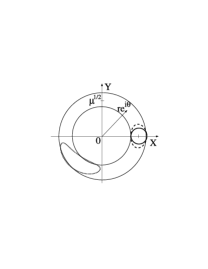
Figure 1: Typical contour plots of the $Q$ function for $\mu=15$ and $C(\equiv\kappa\chi/4\mu)=\kappa(2\pi\mu)^{-1/2}$. Solid ring: stationary laser state $\rho_{\rm ss}$, given by Eq. (23). Solid circle: initial coherent state $|{\sqrt{\mu+1}}\rangle\langle{\sqrt{\mu+1}}|$; dashed contour: phase diffusion due to laser gain and loss at $t\sim 0.8/\kappa$; dotted contour: state due to total evolution including collisions, i.e., Eq. (21), also at $t\sim 0.8/\kappa$.

Substituting Eq. (36) into the expression for magnitude of the first order coherence function (29) gives

$$|g^{(1)}(t)|=e^{-\chi^{2}(e^{-\kappa t}+\kappa t-1)/4\mu}e^{-\kappa t/4\mu},$$ (38)

where we have introduced $\chi=4\mu C/\kappa$ as a dimensionless parameter for the atomic interaction strength. This expression does not have a simple analytical solution. However, by inspection, there are two limits that can be solved analytically. If $\chi\ll\sqrt{\mu}$ we obtain

$$2\tau_{\rm coh}\approx\int_{0}^{\infty}e^{-\kappa(\chi^{2}+1)t/4\mu}dt=4\mu/\kappa(1+\chi^{2}).$$ (39)

For $\chi\gg\sqrt{\mu}$, on the other hand, the first exponential in Eq. (38) is dominant and then expanding $e^{-\kappa t}$ to second order we obtain

$$2\tau_{\rm coh}\approx\int_{0}^{\infty}e^{-\kappa^{2}\chi^{2}t^{2}/8\mu}dt=\sqrt{2\pi\mu}/\kappa\chi.$$ (40)

The resultant expression for the atom laser linewidth due to collisions is thus

$$\ell=\left\{\begin{array}[]{lll}\kappa(1+\chi^{2})/2\mu&~{}{\rm for{}}&\chi\ll\sqrt{\mu}\\ 2\kappa\chi/\sqrt{2\pi\mu}&~{}{\rm for{}}&\chi\gg\sqrt{\mu}\end{array}\right..$$ (41)

Clearly, for $\chi\ll 1$, we obtain the standard laser linewidth $\ell_{0}=\kappa/2\mu$ Lou73 ; SarScuLam74 ; Wis99 . These two expressions agree at $\chi\simeq\sqrt{8\mu/\pi}$, and they are an excellent fit to the numerical calculations of Eq. (24), except at the boundary between the regimes. This is illustrated by the figure in our previous paper WisTho01 , and also the extended version in this paper, Fig. 2 appearing in Sec. III D.

Equation (41) represents the same physical dynamics as found in similar studies by the authors of Refs. ZobMey98 and GarZoll98 . Zobay and Meystre ZobMey98 present a three-mode atom-laser model, with the output mode adiabatically eliminated. Ignoring collisions between pump and laser modes, they obtain phase variances [Eqs. (21) and (22) of Ref. ZobMey98 ], which are similar and identical to the exponents of Eqs. (39) and (40) respectively. See also the linewidth plotted in Fig. 3 of Ref. ZobMey98 . Gardiner and Zoller GarZoll98 studied a Bose-Einstein condensate in dynamical equilibrium with thermal atoms. Our first-order coherence function, Eq. (38), has the same structure as the analogous expression, Eq. (184), derived in Ref. GarZoll98 . The two regimes of Eq. (41) correspond to the characteristic time constants of Eqs. (187) and (186) of Ref. GarZoll98 respectively. The second of these expressions, where the nonlinearity is dominant, is familiar as the inverse collapse time of an initial coherent state in the absence of pumping or damping WriWalGar96 ; ImaLewYou97 .

Since the output power spectrum is the Fourier transform of $G^{(1)}(t)$ [see Eq. (14)], the shape of the spectrum is also determined by the form of $V_{\phi}(t)$. For the two regimes of Eq. (41), the laser output has Lorentzian and Gaussian power spectra respectively, as was also found in Ref. ZobMey98 . These spectra are illustrated by Fig. 6 in Sec. IV B. See Sec. III C for a more in-depth discussion of the atom laser power spectrum.

The standard laser linewidth (in the absence of collisions) is simply given by $\kappa/2\mu$. For the preliminary atom laser experiments of Refs. pulses ; beams , the interaction strength $C$ is always found to satisfy $C\gg\kappa/\mu$ and hence $\chi\gg 1$ WisVac02 . Atom lasers, therefore, have a linewidth far above the standard limit. Furthermore, if $\chi\gtrsim\mu^{3/2}$ the linewidth will be larger than the mean output flux $\kappa\mu$. In other words, the atomic collision strength does not have to become very large before the laser output does not satisfy condition (III) for coherence [i.e., Eq. (13)]. It is thus of great interest to find methods for reducing the linewidth due to atomic interactions. One method is continuous QND measurement and feedback as shown in Sec. IV.

III.4 Revivals of the coherence function

In the preceding section, the atom-laser linewidth was calculated for atom-atom interactions ranging from weak ($\chi\ll 1$) to strong ($\chi\gg\sqrt{\mu}$). However, exact numerical calculations based on Eq. (24) indicated that there is an upper bound to the linewidth (occurring for $\chi\gtrsim\mu^{2}$) that was not included in the previous analysis. It turns out that, in addition to linewidth broadening, the collisional interactions also lead to quantum revivals WriWalGar96 of the first order coherence function. Although, note that in this very strong collisional regime, the output atomic beam cannot be considered a laser according to the definitions in Sec. II (since $\ell\gtrsim\kappa\mu$ for $\chi\gtrsim\mu^{3/2}$).

To study the regime of revivals it is helpful to start by ignoring all other laser dynamics apart from the collisions. In this case, $\dot{\rho}=-iC[a^{\dagger}a^{\dagger}aa]\rho={\cal L}_{C}\rho$, and we can analytically solve for the periodic structure of $g^{(1)}(t)$. For an initial coherent state $\rho(0)=|{\alpha}\rangle\langle{\alpha}|$,

$$g^{(1)}(t)={\rm Tr}[a^{\dagger}\rho(t)]/\alpha^{*},~{}~{}\rho(t)=e^{{\cal L}_{C}t}|{\alpha}\rangle\langle{\alpha}|.$$ (42)

Using the number state representation, i.e. $\rho(t)=\sum p_{mn}(t)|{n}\rangle\langle{m}|$ and $|{\alpha}\rangle=\exp(-|\alpha|^{2}/2)\sum\alpha^{n}|{n}\rangle/\sqrt{n!}$, we find for the first-order coherence function

$$g^{(1)}(t)=\exp\left[{-\mu(1-e^{2iCt})}\right],$$ (43)

since $|\alpha|^{2}=\mu$ for the laser, and its magnitude is

$$|g^{(1)}(t)|=\exp[-\mu(1-\cos 2Ct)].$$ (44)

The coherence function clearly has periodic revivals when $t=m\pi/C$, $m$ is an integer.

Including the other laser dynamics, i.e. gain and loss, is not so straightforward. Since these terms, unlike those in ${\cal L}_{C}$, are not functions of the number operator we cannot easily utilize the number state representation. The main effect, however, is simply a decaying envelope applied to the revivals of Eq. (44), such that the strength of $C$ compared to $\kappa\mu$ will determine the number of significant revivals in the coherence function. This will be shown below. The revivals of the coherence function become significant when $\chi\approx 4\pi\mu^{2}$ or $C\approx\kappa\pi\mu$. This regime was determined by calculating the exact linewidth based on numerical solutions of Eq. (24) and corresponds to the interaction strength where the linewidth begins to approach a maximum.

To determine the value of this maximum linewidth, we extend the work of Milburn and Holmes MilHol86 , who model an anharmonic oscillator coupled to a zero-temperature heat bath, via two basic assumptions for including saturated gain. The master equation modelled by Milburn and Holmes is (using our notation)

$$\dot{\rho}_{\rm MH}=-iC[(a^{\dagger}a)^{2},\rho]+\kappa{\cal D}[a]\rho,$$ (45)

which gives a first-order coherence function of the form

$$g^{(1)}_{\rm MH}(t)=e^{iCt}e^{-\kappa t/2}\exp\left[{-\frac{\mu(1-i\kappa/2C)}{1+\kappa^{2}/4C^{2}}\left({1-e^{2iCt}e^{-\kappa t}}\right)}\right].$$ (46)

To add saturated gain to this model we first assume that, far above threshold, the contribution to phase diffusion is equal for both gain and loss BarStePeg89 and so we replace $\kappa$ with $2\kappa$. Second, including gain will almost cancel the overall exponential decay $e^{-\kappa t/2}$ of the coherence due to loss, resulting in the smaller term $e^{-\kappa t/4\mu}$ (since this will give the standard laser linewidth $\kappa/2\mu$). These assumptions give the following results for $g^{(1)}(t)$ and $|g^{(1)}(t)|$:

$$g^{(1)}(t) \approx e^{iCt}e^{-\kappa t/4\mu}\exp\left[{-\frac{\mu(1-i\kappa/C)}{1+\kappa^{2}/C^{2}}\left({1-e^{2iCt}e^{-2\kappa t}}\right)}\right],$$ (47)

$$|g^{(1)}(t)| \approx e^{-\kappa t/4\mu}\exp\left[{-\frac{\mu}{1+\kappa^{2}/C^{2}}\left({1-e^{-2\kappa t}\cos 2Ct-\frac{\kappa}{C}e^{-2\kappa t}\sin 2Ct.}\right)}\right]$$ (48)

We only expect this expression to be valid in the very strong interaction regime ($C\gg\kappa\mu$). Here revivals of $|g^{(1)}(t)|$ are significant and $\kappa/C\ll 1$ (since $\mu\gg 1$). Also, as shown by Eq. (44), revivals occur at $mt_{r}=m\pi/C$, so in the strong regime the envelope of the coherence function is given by (for finite $m$)

$$|g^{(1)}(t)|_{\rm env} = |g^{(1)}(mt_{r})|\simeq\exp\left\{{-\left({\frac{\kappa}{4\mu}+2\kappa\mu}\right)mt_{r}}\right\}$$ (49)

$$\simeq e^{-2t/t_{Q}},~{}~{}~{}t_{Q}=1/\kappa\mu.$$

Here the time $t_{Q}$ can be interpreted as the quantum dissipation time, i.e. how long the state would last if it was in a superposition of coherent states. Nonunitary effects, such as damping, cause a decay of the quantum coherence of these states at a rate $\propto\kappa\mu$ WalMil85 . This is relevant because the state produced halfway between revivals by nonlinear interactions such as $\cal{L}_{C}$ is in fact a superposition of coherent states DanMil89 .

The relationship between the quantum dissipation time and the revival time can be used to give an indication of the number of significant revivals in the coherence function for a given interaction strength. That is, if $t_{r}\gg t_{Q}$ then no revivals will be seen, but if $t_{r}\ll t_{Q}$ as for the above equation, the number of significant revivals is of order $t_{Q}/t_{r}$. Revivals begin to appear at $t_{r}\simeq t_{Q}$, which is at $\chi\simeq 4\pi\mu^{2}$ or $C\simeq\kappa\pi\mu$ as stated earlier.

We are now in a position to determine coherence time and linewidth in the regime of revivals. From Eq. (10), the coherence time is simply half the area under the function $|g^{(1)}(t)|$. In the very strong interaction regime ($C\gg\kappa\mu$), this area will be made up of many individual peaks which decrease in height due to the envelope given by Eq. (49). The first of these peaks (which actually starts at $|g^{(1)}(0)|=1$) will be the same as the coherence function for no revivals, and its area will be $\sqrt{2\pi\mu}/\kappa\chi$ as given by Eq. (40). The subsequent peaks will have areas twice this area multiplied by the height of the envelope at that time. Thus we have for the total area

$$2\tau_{\rm coh} \simeq \frac{2\sqrt{2\pi\mu}}{\kappa\chi}\left\{{\int_{0}^{\infty}e^{-2t/t_{Q}}\sum_{m=0}^{\infty}\delta(t-mt_{r})dt-\frac{1}{2}}\right\}$$ (50)

$$= \frac{2\sqrt{2\pi\mu}}{\kappa\chi}\left({\sum_{m=0}^{\infty}e^{-2mt_{r}/t_{Q}}-\frac{1}{2}}\right).$$

This expression can be evaluated by using $t_{r}\ll t_{Q}$ and by noting that for a geometric series, $\sum_{m}r^{m}=1/(1-r)$. The analytical expression for the linewidth in the regime of revivals is then

$$\ell_{\rm max}\simeq 4\kappa\sqrt{2\pi}\mu^{3/2}.$$ (51)

This is in exact agreement with the numerical results obtained from Eq. (22), which are plotted Fig. 2.

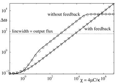
Figure 2: Atom laser linewidth in units of $\kappa$ for $\eta=1$ and $\mu=60$, plotted with and without feedback using both analytical (lines) and numerical (points) methods. The dotted line corresponds to $\ell=\kappa\mu$, i.e. interaction strengths with corresponding linewidths below this line satisfy the coherence condition of Bose degeneracy [condition (III)]. For the feedback results, see Section IV B.

In this figure we have plotted the approximate analytical expressions for the linewidth in the absence [Eqs. (41) and (51)] and presence [Eq. (69)] of feedback (see Sec. IV B for details) as a function of the nonlinearity $\chi$ for $\mu=60$. We have also included numerical results (see Sec. III B for details) as a comparative test for the analytical work, which is valid for $\mu\gg 1$. As can be seen, the agreement is very good even for an occupation number of only 60 fn-compmem , thus confirming the accuracy of our analytical expressions for the linewidth. Without feedback we see four distinct regimes. There is the standard laser linewidth for $\chi\ll 1$, a quadratic dependence on $\chi$ for $1\ll\chi\ll\sqrt{\mu}$, and a linear regime for $\sqrt{\mu}\ll\chi\ll\mu^{2}$. The latter two correspond to the regimes of Eq. (41). Finally there is a constant regime given by Eq. (51) for $\chi\gg\mu^{2}$, which is due to the collapses and revivals of the coherence function.

Note that the approximation used in the numerical calculation of Eq. (24), i.e., $g^{(1)}(t)=|g^{(1)}(t)|e^{i\bar{\omega}t}$, is no longer necessarily valid in the regime of revivals, as indicated by the multi-complex-exponential nature of Eq. (44). Nevertheless, our numerical results are still correct because we have taken the mean atom number $\mu$ to be an integer. At revivals the approximation to $g^{(1)}(t)$ becomes

$$|g^{(1)}(mt_{r})|e^{i\omega_{0}mt_{r}}=|g^{(1)}|e^{i2m\pi\mu},$$ (52)

where we have only used the first guess for $\bar{\omega}$, since the iterative procedure will be inaccurate in this regime (see Appendix B). This expression clearly equals $|g^{(1)}|$ for integer $\mu$. Thus, the same numerical simulation can be used for all values of $C$ as long as $\mu$ is an integer

III.5 Power spectrum

As stated in Sec. II, condition (III) for coherence requires that the integral of $|G^{(1)}(t)|$ be much greater than unity [Eq. (11)]. This was reinterpreted as requiring the linewidth to be much less than the output flux (Bose degeneracy), or equivalently requiring the maximum spectral intensity to be much greater than unity $P(\bar{\omega})\gg 1$. Now the linewidth is only the FWHM of the power spectrum if it is Lorentzian. As discussed after Eq. (41), this will only be the case in the weak-interaction regime $\chi\ll\sqrt{\mu}$. As $\chi$ (or $C$) is increased the power spectrum becomes Gaussian, and as $\chi$ enters the very strong interaction regime it will no longer have a simple structure at all. At these strong values of the nonlinearity we see quantum revivals of $g^{(1)}(t)$.

In terms of normalized first-order coherence function the power spectrum becomes

$$P(\omega)=\kappa\mu\int_{-\infty}^{\infty}g^{(1)}(t)e^{-i\omega t}dt,$$ (53)

where we have recognized that $\left\langle{I}\right\rangle=\left\langle{b^{\dagger}b}\right\rangle=\kappa\left\langle{a^{\dagger}a}\right\rangle=\kappa\mu$. From this equation it is clear that as long as $g^{(1)}(t)$ has a simple structure, i.e., no revivals, then the spectrum will have a simple (Lorenztian or Gaussian) lineshape for a given interaction strength $C$, with the intensity and width determined by how fast $g^{(1)}(t)$ decays.

The maximum spectral intensity was defined in Sec. II by Eq. (15), which was based on the assumption that $g^{(1)}(t)=|g^{(1)}(t)|e^{i\bar{\omega}t}$. Since we are in a reference frame with zero mean frequency before including collisions, $\bar{\omega}$ is the detuning frequency due to collisions which causes the mean phase shift of an initial coherent state (see Fig. 1). At this frequency, the output power spectrum will, therefore, have a maximum value given by

$$P(\bar{\omega})=4\kappa\mu\tau_{\rm coh}.$$ (54)

As stated above, in the regime of revivals this approximation will only be accurate for the first guess for $\bar{\omega}$, i.e., $\omega_{0}=2\mu C$.

The linewidth in the strong atomic interaction regime ($C\gtrsim\kappa\pi\mu$) was calculated in the preceding section to be $4\kappa\sqrt{2\pi}\mu^{3/2}$, i.e. Eq. (51). Thus, from the above equation, we expect the maximum spectral intensity to reach

$$P(\omega_{0})=4\kappa\mu/\ell_{\rm max}=1/\sqrt{2\pi\mu},$$ (55)

as the atomic interaction strength $C$ is increased far above $\kappa\pi\mu$.

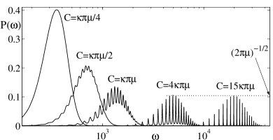
Figure 3: Output power spectrum $P(\omega)$ where $\omega$ has units of $\kappa$, plotted for $\mu=15$ and various values of $C$ in the strong interaction regime. The dotted line corresponds to the value $4\kappa\mu/\ell_{\rm max}$, i.e., the maximum height of the power spectrum in the regime of revivals. Note the log scale for $\omega$.

Figure 3 illustrates both the simple lineshape of the power spectrum when there are no revivals and the complication of the spectrum as $C$ is increased. Since all the plotted spectra have $P(\bar{\omega})<1$, the atom-laser output clearly does not satisfy condition (III) for coherence, Eq. (16), in the strong interaction regime. The first spectrum in Fig. 3 is in the range $\sqrt{\mu}<C<\kappa\pi\mu$, and thus although revivals are not seen, the output is still above the cutoff for Bose degeneracy.

The remaining spectra illustrate the increasing effect of quantum revivals due to increasing interaction strength. The central peak of the power spectrum, which can be defined regardless of revivals as shown in Eq. (15), clearly approaches the predicted maximum of $1/\sqrt{2\pi\mu}$, i.e., Eq. (55), for $C\gg\kappa\pi\mu$. For examples of the spectrum in the weak interaction regimes of Eq. (41), see Sec. IV B.

IV Reducing the linewidth via feedback

Section III A showed that the atomic interactions do not directly cause phase diffusion. Rather, they cause a shearing of the field in phase space, with higher amplitude fields having higher energy and hence rotating faster. The resultant linewidth broadening is a known effect for optical lasers with a Kerr ($\chi^{(3)}$) medium Watetal90 . The shearing of the field is manifest in the finite value acquired by the covariance $C_{n\phi}(t)$ in Eq. (37). It means that information about the condensate number is also information about the condensate phase. Hence, we can expect that feedback based on atom number measurements could enable the phase dynamics to be controlled, and the linewidth reduced.

IV.1 QND feedback scheme

QND atom number measurements can be performed on the condensate in situ via the homodyne detection of a far-detuned probe field Andetal96 ; CorMil98 ; Lyeetal99 ; Daletal01 . This dispersive interaction causes a phase shift of the probe proportional to the number of atoms in the condensate. We consider a far-detuned probe laser beam of frequency $\omega_{p}$ and cross-sectional area $A$ that passes through the condensate fn-antimean . Figure 4 shows an experimental schematic for our QND measurement and feedback scheme.

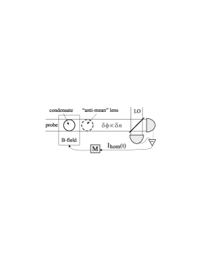
Figure 4: Experimental schematic. A far-detuned probe laser of amplitude $\varrho$ interacts with the condensate (i.e., the laser cavity) causing a phase shift in the probe proportional to the condensate number. The “anti-mean” lens subtracts the mean phase shift leaving the probe with a phase shift proportional to the number fluctuations $\delta n$. The photocurrent $I_{\rm hom}(t)$ from the homodyne $Y$ detection of this field is then used to modulate an external $B$-field uniformly applied to the condensate.

For a single atom the interaction with the optical probe field can be approximated by the Hamiltonian

$$V=\hbar\frac{\Omega_{p}^{2}}{4\Delta}=\hbar\left(\frac{\hbar\omega_{p}\gamma^{2}}{8A\Delta I_{\rm sat}}\right)p^{\dagger}p\equiv\hbar\theta p^{\dagger}p,$$ (56)

where $\Omega_{p}$, $\Delta$, $\gamma$ have their usual meaning and $I_{\rm sat}=2\pi hc\gamma/\lambda^{3}$ Ash70 . Here $p$ is the annihilation operator for the probe beam, normalized so that $\hbar\omega_{p}p^{\dagger}p$ is the beam power.

The effective interaction Hamiltonian for the whole condensate can thus be taken to be

$$H_{\rm int}=\hbar\theta(a^{\dagger}a-\mu)p^{\dagger}p,$$ (57)

where $\theta$, defined in Eq. (56), is the phase shift of the probe field due to a single atom. Here we have also subtracted the mean phase shift such that the probe optical laser is a measure of the atom number fluctuations only (see Fig. 4).

The back action on the condensate due to this interaction can be evaluated using the techniques of Sec. III B of Ref. Wis94 . Assuming the input probe field is in a coherent state of amplitude $\varrho$ and mean power $P$, the evolution of the atomic system due the measurement is

$$\dot{\rho}=\varrho^{2}{\cal D}[e^{-i\theta(a^{\dagger}a-\mu)}]\rho\simeq M{\cal D}[a^{\dagger}a]\rho,$$ (58)

where the the measurement strength is given by

$$M=\varrho^{2}\theta^{2}=P\theta^{2}/\hbar\omega_{p}.$$ (59)

The approximation in Eq. (58) requires $\theta(a^{\dagger}a-\mu)\ll 1$, which for Poissonian number fluctuations is simply $\sqrt{\mu}\theta\ll 1$.

The above result represents decoherence of the atom laser due to photon number fluctuations in the probe field, resulting in increased phase noise. In a recent theoretical study by Dalvit and co-workers Daletal01 , it was shown that dispersive measurements of BECs cause both phase diffusion [as in Eq. (58)] and atom losses. Nevertheless, they also show that phase diffusion dominates the decoherence rate for large atom numbers, i.e., for $\mu\gg 1$, and so the depletion contribution can generally be neglected fn-depletion . Equation (58) is equivalent to the corresponding phase diffusion term in their work, since it can be shown that both $M$ and the phase diffusion rate given by Eq. (14) of Daletal01 reduce to $\sim\gamma^{2}\lambda^{5}I/hcA\Delta^{2}$.

The effect of the interaction (57) on the output probe field is to cause a phase shift proportional to the number fluctuations, $a^{\dagger}a-\mu$. The output field operator is given by Wis94

$$p_{\rm out}=e^{-i\theta(a^{\dagger}a-\mu)}p_{\rm in}\simeq p_{\rm in}-i\varrho\theta(a^{\dagger}a-\mu),$$ (60)

where again the approximation requires $\sqrt{\mu}\theta\ll 1$. Homodyne detection of the $Y$ quadrature of the output probe field will thus be a measure of the condensate number fluctuations. The homodyne photocurrent operator is given by Wis94

$$I^{\rm Y}_{\rm out}=-ip_{\rm out}+ip_{\rm out}^{\dagger}\simeq I^{\rm Y}_{\rm in}-2\sqrt{M}(a^{\dagger}a-\mu).$$ (61)

In order to control the phase dynamics of the condensate, we wish to use this homodyne current to modulate its energy. This can be done, for example, by applying a uniform magnetic field or far-detuned light field across the whole condensate. In the ideal limit of instantaneous feedback, we model this by the Hamiltonian

$$H_{\rm fb}(t)=-\hbar a^{\dagger}aFI_{\rm hom}(t)/\sqrt{M},$$ (62)

where $F$ is the feedback strength and $I_{\rm hom}(t)$ is the classical photocurrent corresponding to the operator $I^{\rm Y}_{\rm out}$.

The total evolution of the system including feedback is obtained by applying the Markovian theory of Ref. Wis94 . The master equation becomes

$$\dot{\rho} = {\cal L}_{0}\rho-iC[a^{\dagger}a^{\dagger}aa,\rho]+M{\cal D}[a^{\dagger}a]\rho$$ (63)

$${+}\,iF[a^{\dagger}a^{\dagger}aa,\rho]+\frac{F^{2}}{\eta M}{\cal D}[a^{\dagger}a]\rho,$$

where we have allowed for a detection efficiency $\eta$ Wis94 and dropped terms corresponding to a frequency shift.

The terms in Eq. (63) describe, respectively, the standard laser gain and loss (${\cal L}_{0}$), the collisional interactions ($C$), the measurement back action ($M$), the feedback phase alteration ($F$), and the noise introduced by the feedback. As before we can visualize the effect of the measurement and feedback terms on the evolution of an arbitrary coherent state. This is illustrated by the $Q$-function contours in Fig. 5. In this figure we have ignored the mean phase shift due to collisions to make the comparison clearer.

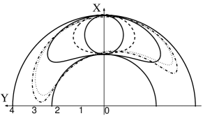
Figure 5: Contour plots of the $Q$ function for $\mu=10$ and $C=\kappa(2\pi\mu)^{-1/2}$ (ignoring any mean phase shifts). Black circle: initial coherent state $|{\sqrt{\mu}}\rangle\langle{\sqrt{\mu}}|$; black ring: stationary laser state $\rho_{\rm ss}$, Eq. (23). The other contours correspond to the evolution at time $t\sim 1.5/\kappa$ due to successive terms in the master equation. Dashed contour: phase diffusion due to ${\cal L}_{0}$; dotted contour: including atomic collisions, i.e., ${\cal L}_{0}$ and $C$; dot-dash contour: including QND measurement back action, i.e., ${\cal L}_{0}$ and $C$ and $M$, and finally the solid contour corresponds to Eq. (64). All contours are for the optimal feedback regime $F=\sqrt{\eta}M=C$.

To completely remove that unwanted nonlinearity, the obvious choice for the feedback strength is $F=C$. We also want to minimize the phase diffusion introduced by both the measurement and feedback. A weak measurement will give poor information about the atom number, with a high noise-to-signal ratio, which will increase the noise due to feedback. On the other hand, if the measurement is too strong the measurement back action itself will dominate. This leads us to guess the optimal regime for both measurement and feedback to be $F=\sqrt{\eta}M=C$, which simply leaves

$$\dot{\rho}=\kappa\mu{\cal D}[a^{\dagger}]{\cal A}[a^{\dagger}]^{-1}\rho+\kappa{\cal D}[a]\rho+\frac{2C}{\sqrt{\eta}}{\cal D}[a^{\dagger}a]\rho.$$ (64)

IV.2 Linewidth results

Proceeding as before, we can find the exact effect of the general feedback scheme on the atom-laser linewidth. Neither the measurement nor the feedback affect the atom number statistics. The change in the phase statistics are reflected by the new Fokker-Planck equation for $Q(n,\phi)$. The altered terms in the drift vector and diffusion matrix are $A_{2}=(3-2n)(C-F)$, $B_{12}=B_{21}=2n(C-F)$, and $B_{22}=\kappa/2n+M+F^{2}/\eta M$. After linearizing, we again find the phase-related moments:

$$\bar{\phi}(t) \simeq -2\mu(C-F)t,$$ (65)

$$V_{\phi}(t) \simeq \frac{8\mu(C-F)^{2}}{\kappa^{2}}\left({e^{-\kappa t}+\kappa t-1}\right)$$ (66)

$${+}\,\left({\frac{\kappa}{2\mu}+M+\frac{F^{2}}{\eta M}}\right)t,$$

$$C_{n\phi}(t) \simeq \frac{2\mu(C-F)}{\kappa}\left({e^{-\kappa t}-1}\right),$$ (67)

where again the approximations have used $\mu\gg 1$.

These equations clearly show that all the unwanted phase statistics are cancelled by choosing a feedback regime with $F=C$ and furthermore the minimum phase variance is when $M=C/\sqrt{\eta}$. Specifically, both the mean phase shift and the correlation between number and phase fluctuations are removed, and the phase variance is simply given by

$$V_{\phi}(t)=\left({\frac{\kappa}{2\mu}+\frac{2C}{\sqrt{\eta}}}\right)t.$$ (68)

This is exactly the phase variance from the master equation (64).

In this case, Eq. (30) has a simple analytical solution:

$$\ell=\tau_{\rm coh}^{-1}=\frac{\kappa}{2\mu}\left({1+\frac{\chi}{\sqrt{\eta}}}\right),$$ (69)

where we have again used the dimensionless atomic interaction strength $\chi=4\mu C/\kappa$. Note that unlike Eq. (41), this linewidth is valid for all $\chi$. The derivation of Eq. (69) above is based on preselecting the feedback and measurement parameters (i.e., $F=\sqrt{\eta}M=C$). On the other hand, Ref. WisTho01 presented the analytical solution for the linewidth independent of the choice of these parameters and proceeded to find the minimum with respect to the feedback strength. The result [Eq. (24) of Ref. WisTho01 ] only differs from Eq. (69) by the term $\kappa(-1/4\eta)/2\mu$.

From Fig. 2 (in Sec. III C) and the above result, Eq. (69), it is evident that our QND feedback scheme offers a linewidth much smaller than that without feedback for most values of $\chi$. In fact for $\sqrt{\mu}\lesssim\chi\lesssim 4\pi\mu^{2}$ the reduction in linewidth due to feedback is a factor of $\sqrt{8\mu/\pi}$. Most importantly, the laser output is Bose degenerate [satisfies condition (III) for coherence], up to $\chi\approx\mu^{2}$ with feedback, as opposed to $\chi\approx\mu^{3/2}$ in the absence of feedback. Thus, the atom laser with feedback remains coherent for much stronger atomic nonlinearities than without feedback. It is interesting that this corresponds to the “conditionally coherent” regime $\mu^{3/2}<\chi<\mu^{2}$ as discussed in Ref. WisVac02 .

Since the nonlinearity $C$ is effectively cancelled by this feedback scheme, the output power spectrum, Eq. (53), will never have the complicated structure as shown in Sec. III C. Also, since Eq. (68) has a linear dependence on time (rather than higher powers) the first-order coherence function decays exponentially and as such will produce a Lorentzian output power spectrum [see discussion after Eq. (14)].

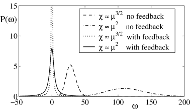
Figure 6: Output power spectrum $P(\omega)$ for $\mu=15$ vs $\omega$ in units of $\kappa$, plotted with and without feedback for interaction strengths of $\chi=\mu^{3/2}$ and $\chi=\mu^{2}$. The dotted spectrum ($\chi=\mu^{3/2}$ with feedback) has a maximum intensity of $\sim 31$.

This lineshape is illustrated in Fig. 6, which also plots the corresponding spectra that would be produced by the laser (for the same values of $\chi$) without feedback. These latter spectra have a Gaussian lineshape as discussed after Eq. (41). Also, as indicated by Eq. (65), the rotation of the mean phase due to collision is cancelled by our feedback scheme, i.e., $g^{(1)}(t)$ is no longer complex and hence $\bar{\omega}=0$. The power spectrum for the atom laser including feedback will thus be centered around zero frequency regardless of the atomic interaction strength, which is confirmed in the figure.

The spectra in Fig. 6 are plotted at the two cutoff values for Bose degeneracy, which are $\chi\approx\mu^{3/2}$ for no feedback and $\chi\approx\mu^{2}$ when feedback is included. If the output is coherent, i.e., satisfies Bose degeneracy, then it clearly has a much narrower and thus more intense spectrum than if the output is not coherent. This figure thus illustrates the link between the three definitions of linewidth [discussed after Eq. (15)] and its relation to coherence. That is, a narrow intense output spectral line corresponds to a long phase coherence time, and more specifically, if the FWHM linewidth is much less than the value of the output flux, then the laser output will satisfy the conditions of coherence.

IV.3 Experimental realizability

We will now briefly examine some issues of experimental realizability. A question of interest is, how easy is it to obtain a QND measurement of sufficient strength to optimize the feedback? We have shown in Sec. IV B that the optimum feedback scheme requires $N=C/\sqrt{\eta}$. From Ref. WisVac02 we know that most current experiments work in the regime where the Thomas-Fermi approximation can be made, allowing an analytical expression to be found for $\chi$ [Eq. (6.25) in WisVac02 ] and $C$. Typical values are $\chi\sim 10^{3}$, $\mu\sim 10^{6}$ and $C\sim 10^{-2}$s^-1. To determine $\theta$ and hence $M$ we use typical ⁸⁷Rb imaging parameters Lyeetal99 ; Daletal01 , which include $\lambda=780$nm, $A\sim 10^{-11}$m², $\gamma\sim 5$Mhz, $\Delta\sim 2$GHz, and $I_{\rm sat}\sim 10$W$/$m². For these values, $\theta\sim 3.3\times 10^{-6}$, and thus $M\sim 4.2\times 10^{-4}\times I$. To obtain a measurement strength of the order of $C$, we therefore require a probe laser intensity of only $\sim 30$W/m², which is quite reasonable.

A related question is, how much of a problem is atom loss due to spontaneous emission by atoms excited by the detuned probe beam? The rate of this loss (ignoring reabsorption) is $\gamma\times(\textrm{excited population})$. We would like the ratio of this loss rate to the output loss rate $\kappa\mu$ to be small. In the optimal feedback regime and for $\Delta\gg\gamma$, this ratio is given by

$$\frac{\gamma\mu\Omega_{p}^{2}/4\Delta^{2}}{\kappa\mu}=\frac{4\mu M}{\kappa}\frac{2AI_{\rm sat}}{\hbar\omega_{p}\gamma\mu}\approx\chi\frac{2AI_{\rm sat}}{\hbar\omega_{p}\gamma\mu}.$$ (70)

For the typical values stated above, Eq. (70) is indeed small ($\sim 10^{-1}$).

Another practical question is, how realistic is the zero-time-delay assumption for the feedback? It can be shown using the techniques of Ref. Wis94 that this assumption is justified providing the feedback delay time is much less than $\kappa^{-1}$, the lifetime of the trap due to the output coupling. If recent experiments pulses ; beams are a useful guide, trap lifetimes are of order $10^{-2}$s WisVac02 . Feedback much faster than this should not be a problem. In fact, the time delay could be completely eliminated by feeding forward rather than feeding back. Linewidth reduction can be achieved equally well by controlling the phase of the atom field once it has left the trap as by controlling it inside the trap (but, of course, an integrated, rather than instantaneous, current would be used for the control).

V Summary

The coherence of an atom laser can be defined Wis97 analogously to that of an optical laser: it should be monochromatic with small intensity and phase fluctuations. We used the normalized first-order coherence function $g^{(1)}(t)=G^{(1)}(t)/\left\langle{I}\right\rangle$ Glau63 as a measure of the phase fluctuations. As $t$ increases, $|g^{(1)}(t)|$ decreases from unity as the phase of the field becomes decorrelated from its initial value. Its decay is characterized by the coherence time $\tau_{\rm coh}=\frac{1}{2}\int_{0}^{\infty}|g^{(1)}(t)|dt$, or by its reciprocal, the linewidth $\ell$. $G^{(1)}(t)$ also determines the output power spectrum, where the peak spectral height is given by $4\left\langle{I}\right\rangle/\ell$ regardless of lineshape, while for a Lorentzian the FWHM is also equal to $\ell$.

We examined the linewidth as a function of the dimensionless atomic interaction strength, $\chi=4\mu C/\kappa$, where $\kappa$ is the output coupling rate and $C$ is the atomic self-energy. There are four distinct regimes: the standard laser linewidth for $\chi\ll 1$, a quadratic dependence on $\chi$ for $1\ll\chi\ll\sqrt{\mu}$, a linear regime for $\sqrt{\mu}\ll\chi\ll\mu^{2}$, and finally another constant regime when $\chi\gg\mu^{2}$. The second and third regimes have Lorentzian and Gaussian output spectra respectively. The last regime is a consequence of quantum revivals of $|g^{(1)}(t)|$, which are a direct effect of strong atomic collisions WriWalGar96 . This leads to a complicated structure in the power spectrum with many peaks contained in a Gaussian-like envelope.

An important condition for atom-laser coherence is that the phase fluctuations be small in a particular sense. This is equivalent to requiring Bose degeneracy in the output, i.e., that the linewidth $\ell$ be much less than the the output flux $\left\langle{I}\right\rangle=\kappa\mu$. From the results presented here, this means that the laser output is only coherent for interaction strengths satisfying $\chi\lesssim\mu^{3/2}$, i.e., somewhere in the third linewidth regime. Therefore, collisions will be a problem for atom-laser coherence, especially for BECs formed by evaporative cooling where collisions are the dominant mechanism. On the other hand, if the atom-atom interactions are strong enough, the laser output will exhibit the interesting feature of quantum revivals.

We also show, expanding upon Ref. WisTho01 , that this linewidth broadening can be significantly reduced by a QND feedback scheme. Basically, by feeding back the results of a QND measurement of the number fluctuations to control the condensate energy, it is possible to compensate for the linewidth caused by the frequency fluctuations. The very number-phase correlation created by the collisions is utilized to cancel their effect. We have shown that this linewidth reduction allows the output to remain coherent for interaction strengths up to $\chi\simeq\mu^{2}$ rather than $\mu^{3/2}$, which is an improvement by a factor of $\sqrt{\mu}$. For the reasonable parameters of $C\sim 10^{-2}s^{-1}$ and $\mu\sim 10^{6}$, this improvement in linewidth is of the order of $10^{3}$ and in principle could increase coherent values of $\chi=4\mu C/\kappa$ from $\sim 10^{9}$ to $\sim 10^{12}$.

Appendix A Single complex exponential approximation for $g^{(1)}(t)$

For the majority of the calculations in this paper we assume that the first order coherence function can be given by

$$g^{(1)}(t)=|g^{(1)}(t)|e^{i\bar{\omega}t}.$$ (71)

That is, we assume that the complex nature of $g^{(1)}(t)$ (which is due only to collisions as shown in Sec. III D) is described by a single complex exponential for most regimes of the collisional nonlinearity. When the collisions are strong enough to cause revivals this approximation necessarily breaks down.

To determine the relative error caused by this approximation we continue the analysis of evolution due to collisions presented in Sec III D, i.e., for $\dot{\rho}={\cal L}_{C}\rho$. Specifically, we quantify the relative difference between

$$\tau_{\rm exact}=\frac{1}{2}\int_{0}^{\infty}e^{-\mu(1-\cos 2Ct)}dt$$ (72)

and

$$\tau_{\rm approx}=\frac{1}{2}\int_{0}^{\infty}e^{-\mu[1-\exp(2iCt)]-i\bar{\omega}t}dt.$$ (73)

This is done by multiple Taylor expansions [first of $\cos 2Ct$ and $\exp(2iCt)$, and then expanding resultant exponentials apart from $\exp(at^{2})$] and using the equality

$$\int_{0}^{\infty}t^{n}e^{-2\mu C^{2}t^{2}}dt=\frac{\Gamma[(n+1)/2]}{2(2\mu C^{2})^{(n+1)/2}},$$ (74)

where $\Gamma[n]$ is the Gamma function.

Now, $\tau_{\rm approx}$ differs from $\tau_{\rm exact}$ by both real and imaginary terms. The dominant [for $t<(\mu C^{2})^{-1/2}$] real term is

$$-\frac{(2\mu C-\bar{\omega})^{2}}{32}\sqrt{\frac{\pi}{2}}\left({\frac{1}{\mu C^{2}}}\right)^{3/2}+...$$ (75)

while the first three imaginary terms are

$$\frac{(2\mu C-\bar{\omega})}{8\mu C^{2}}-\left[{\frac{2}{3}\mu C^{3}+\frac{1}{12}(2\mu C-\bar{\omega})^{3}}\right]\frac{1}{8(\mu C^{2})^{2}}+...$$ (76)

We can thus determine $\bar{\omega}$ by requiring that the imaginary terms vanish. This is essentially what the iterative procedure of Appendix B achieves.

The series of imaginary terms above leads to a first choice of $\omega_{0}=2\mu C$, i.e., this sets the first term to zero and we are left with terms of ${\cal O}[(\mu C)^{-1}]$. To cancel the first two imaginary term we require $2\mu C-\bar{\omega}=2C/3$, leaving terms of ${\cal O}[(\mu^{2}C)^{-1}]$. Hence, $\omega_{1}=2\mu C-2C/3$ will largely ensure that $\tau_{\rm approx}$ is real (since $\mu\gg 1$). The question now is, how much different is $\tau_{\rm approx}$ from $\tau_{\rm exact}$ using $\omega_{1}$?

The dominant term in the difference is simply found by substituting $\omega_{1}$ into Eq. (75), giving

$$\frac{1}{36\mu^{3/2}C}\sqrt{\frac{\pi}{2}}.$$ (77)

The relative size of this error term is obtained by comparing to $\tau_{\rm exact}$, which using the Taylor expansion equals

$$\tau_{\rm exact}\simeq\frac{1}{2}\int_{0}^{\infty}e^{-2\mu C^{2}t^{2}}dt=\frac{1}{4\mu^{1/2}C}\sqrt{\frac{\pi}{2}}.$$ (78)

This corresponds to a relative error, given by $(\tau_{\rm approx}-\tau_{\rm exact})/\tau_{\rm exact}$, of the order of $\mu^{-1}$. We have also verified the size of this error numerically for the full system dynamics by simulations of $|g^{(1)}(t)|$ and $g^{(1)}(t)\exp(-i\omega_{1}t)$ (here $\omega_{1}$ is found in the same way as shown in Appendix B). These results also confirmed that the single complex exponential approximation breaks down when $C\sim\kappa\pi\mu$ (or $\chi\sim 4\pi\mu^{2}$), as expected.

Appendix B Iterative procedure for the coherence time $\tau_{\rm coh}$

As stated in Sec. III B, the coherence time can be evaluated numerically using Eq. (24), where the first guess for $\bar{\omega}$ is given by Eq. (25). Subsequent corrections to $\bar{\omega}$ are found by applying the procedure:

$$\tau_{k} =~{}-{{\rm Tr}[a^{\dagger}({\cal L}-i\omega_{k})^{-1}a\rho_{\rm ss}]}/2\left\langle{a^{\dagger}a}\right\rangle,$$ (79)

$$\omega_{k+1} =~{}\omega_{k}-{\rm Im}(1/2\tau_{k}).$$

At each step we have

$$2\tau_{k}=\int_{0}^{\infty}g^{(1)}(t)e^{-i\omega_{k}t}dt,$$ (80)

which is simply a reexpression of Eq. (79). Then using the assumption of Appendix A that $g^{(1)}(t)\approx|g^{(1)}(t)|e^{i\bar{\omega}t}$, we have

$$2\tau_{k}\approx\int_{0}^{\infty}|g^{(1)}(t)|e^{i(\bar{\omega}-\omega_{k})t}dt.$$ (81)

The simplest form for $|g^{(1)}(t)|$ is a decaying exponential, $\exp(-\gamma t)$, which gives rise to a Lorentzian power spectrum as discussed at the end of Sec. II. In this case

$$2\tau_{k}\approx\int_{0}^{\infty}e^{-[\gamma-i(\bar{\omega}-\omega_{k})]t}dt=\frac{1}{\gamma-i(\bar{\omega}-\omega_{k})},$$ (82)

and hence

$${\rm Im}(1/2\tau_{k})\approx\omega_{k}-\bar{\omega}.$$ (83)

The more complicated form of $|g^{(1)}(t)|=\exp(-\gamma^{2}t^{2})$, which gives rise to a Gaussian power spectrum, also obeys Eq. (83), since in this case

$$2\tau_{k} \approx \int_{0}^{\infty}e^{-[\gamma^{2}t^{2}-i(\bar{\omega}-\omega_{k})t]}dt$$ (84)

$$= \frac{\sqrt{\pi}}{2\gamma}~{}e^{-(\bar{\omega}-\omega_{k})^{2}/4\gamma^{2}}~{}{\rm erfc}\left[{\frac{-i(\bar{\omega}-\omega_{k})}{2\gamma}}\right]$$

$$\simeq -1/i(\bar{\omega}-\omega_{k}).$$

Thus, if the coherence function is in the regime where the output spectrum is Lorentzian or Gaussian, then $\omega_{k+1}\approx\bar{\omega}$, and the first correction, $\omega_{1}$, will be sufficient for an accurate calculation. On the other hand, if the coherence function is in the regime of revivals then the approximation $g^{(1)}(t)\approx|g^{(1)}(t)|e^{i\bar{\omega}t}$ itself is no longer valid. Therefore, the above numerical method will be wildly inaccurate and we require another method for obtaining the coherence time and linewidth. This is detailed in Sec. III D.

Appendix C Q-function correspondence for saturated gain

As stated in Sec. III C the master equation can be reexpressed as a Fokker-Planck equation for a convenient probability distribution. In this appendix we show that, for the Q function, the operator correspondence for the gain term is given by Eq. (32). The individual superoperators in this expression have the corresponding differential operators,

$${\cal D}[a^{\dagger}]\rho \to -\frac{\partial}{\partial{n}}n~{}Q(n,\varphi),$$ (85)

$${\cal A}[a^{\dagger}]\rho \to \left({n+\frac{\partial}{\partial{n}}n}\right)Q(n,\varphi).$$ (86)

Combining these leads to the following correspondence for the saturated gain term:

$${\cal D}[a^{\dagger}]{\cal A}[a^{\dagger}]^{-1}\rho~{}\to-\frac{\partial}{\partial{n}}n\left({n+\frac{\partial}{\partial{n}}n}\right)^{-1}Q(n,\varphi),$$ (87)

which can be expanded in two different ways to give

$$\left\{{\left({1+\frac{1}{n}\frac{\partial}{\partial{n}}n}\right)^{-1}-1}\right\}Q(n,\varphi),$$ (88)

or

$$-\frac{\partial}{\partial{n}}\left({1+\frac{1}{n}\frac{\partial}{\partial{n}}n}\right)^{-1}Q(n,\varphi).$$ (89)

Equating these expressions leads to

$$\left({1+\frac{1}{n}\frac{\partial}{\partial{n}}n}\right)^{-1}=\left({1+\frac{\partial}{\partial{n}}}\right)^{-1},$$ (90)

and hence

$${\cal D}[a^{\dagger}]{\cal A}[a^{\dagger}]^{-1}\rho~{}\to~{}\left\{{\left({1+\frac{\partial}{\partial{n}}}\right)^{-1}-1}\right\}Q(n,\varphi).$$ (91)

By then applying the Taylor expansion, $(1+x)^{-1}=\sum_{k=0}^{\infty}(-x)^{k}$, we obtain the identity

$${\cal D}[a^{\dagger}]{\cal A}[a^{\dagger}]^{-1}\rho~{}\to~{}\sum_{k=1}^{\infty}\left({-\frac{\partial}{\partial{n}}}\right)^{k}Q(n,\varphi).$$ (92)

References

- (1) A. L. Schawlow and C. H. Townes, Phys. Rev. 112, 1940 (1958).
- (2) K. Helmerson, D. Hutchinson, K. Burnett, and W. D. Phillips, Phys. World 12(8), 31 (1999); W. Ketterle, Phys. Today 52(12), 30 (1999).
- (3) C. S. Adams, M. Sigel, and J. Mlynek, Phys. Rep. 240, 145 (1994).
- (4) H. M. Wiseman, Phys. Rev. A 56, 2068 (1997).
- (5) Of course, some optical lasers have a pulsed rather than continuous output. However, as argued in Ref. Wis97 , in order for the term “atom laser” to mean something more than merely an atomic Bose-Einstein condensate released from its trap, it is useful to impose the condition that a true atom laser has a continuous output.
- (6) M. H. Anderson et al., Science 269, 198 (1995); K. B. Davis et al., Phys. Rev. Lett. 75, 3969 (1995); C. C. Bradley, C. A. Sackett, J. J. Tollett, and R. G. Hulet, ibid. 75, 1687 (1995).
- (7) M. Olshanii, Y. Castin, and J. Dalibard, in Proceedings of the XII Conference on Lasers Spectroscopy, edited by M. Inguscio, M. Allegrini and A. Sasso (World Scientific, Singapore, 1995); R. J. C. Spreeuw, T. Pfau, U. Janicke, and M. Wilkens, Europhys. Lett. 32, 469 (1995); H. M. Wiseman and M. J. Collett, Phys. Lett. A 202, 246 (1995); A. M. Guzman, M. Moore, and P. Meystre, Phys. Rev. A 53, 977 (1996); M. Holland et al, ibid. 54, R1757 (1996).
- (8) M.-O. Mewes et al., Phys. Rev. Lett. 78, 582 (1997); B. P. Anderson and M. A. Kasevich, Science 282, 1686 (1998); J. L. Martin et al., J. Phys. B 32, 3065 (1999).
- (9) E.W. Hagley et al., Science 283, 1706 (1999); I. Bloch, T. W. Hänsch, and T. Esslinger, Phys. Rev. Lett. 82, 3008 (1999); Nature 403, 166 (2000).
- (10) H. M. Wiseman, A.-M. Martins, and D. F. Walls, Quantum Semiclassical Opt. 8, 737 (1996); G. M. Moy, J. J. Hope, and C. M. Savage, Phys. Rev. A 55, 3631 (1997); M. Edwards et al., J. Phys. B 32, 2935 (1999).
- (11) M. Köhl, T. W. Hänsch, and T. Esslinger, Phys. Rev. Lett. 87, 160404 (2001).
- (12) S. Dettmer et al., Phys. Rev. Lett. 87, 160406 (2001).
- (13) Y. Le Coq et al., Phys. Rev. Lett. 87, 170403 (2001).
- (14) R. J. Dodd at al., Opt. Express 1, 284 (1997).
- (15) O. Zobay and P. Meystre, Phys. Rev. A 57, 4710 (1998).
- (16) E. V. Goldstein, O. Zobay, and P. Meystre, Phys. Rev. A 58, 2373 (1998).
- (17) M. W. Jack, M. Naraschewski, M. J. Collett, and D. F. Walls, Phys. Rev. A 59, 2962 (1999).
- (18) J. J. Hope, G. M. Moy, M. J. Collett, and C. M. Savage, Phys. Rev. A 61, 023603 (2000).
- (19) N. Robins, C. Savage, and E. A. Ostrovskaya, Phys. Rev. A 64, 043605 (2001).
- (20) H. M. Wiseman and L. K. Thomsen, Phys. Rev. Lett. 86, 1143 (2001).
- (21) L. D. Landau, E. M. Lifshitz, and L. P. Pitaevskii, Statistical Physics, (Pergamon Press, Oxford, 1980).
- (22) D. F. Walls and G. J. Milburn, Quantum Optics, (Springer Verlag, Berlin, 1994).
- (23) Although there have been some recent ideas on how to tackle this [J. J. Hope (private communication)].
- (24) K. Mølmer, Phys. Rev. A 55, 3195 (1997).
- (25) R. J. Glauber, Phys. Rev. 130, 2529 (1963).
- (26) A. S. Holevo, Lect. Notes Math. 1055, 153 (1984).
- (27) Based on an input-output formalism for atoms, the time dependence of the output spectrum has also been calculated inout97 , where the power spectrum defined in Eq. (14) is simply the steady-state limit.
- (28) J. J. Hope, Phys. Rev. A 55, R2531 (1997); G. M. Moy and C. M. Savage, ibid. 56, R1087 (1997).
- (29) H. M. Wiseman, Phys. Rev. A 60, 4083 (1999).
- (30) W. H. Louisell, Quantum Statistical Properties of Radiation (Wiley, New York, 1973).
- (31) M. Sargent, M. O. Scully, and W. E. Lamb, Laser Physics (Addison-Wesley, Reading, MA, 1974).
- (32) C. W. Gardiner, Quantum Noise (Springer-Verlag, Berlin, 1991).
- (33) R. J. Ballagh and C. M. Savage, in Proceedings of the XIII Physics Summer School, Boes-Einstein Condensation, edited by C. M. Savage, M. P. Das (World Scientific, Singapore, 2000).
- (34) H. M. Wiseman and J. A. Vaccaro, Phys. Rev. A 65, 043605 (2002).
- (35) H. M. Wiseman and J. A. Vaccaro, Phys. Rev. Lett. 87, 240402 (2001).
- (36) S. M. Tan, J. Opt. B: Quantum Semiclassical Opt. 1, 424 (1999).
- (37) C. W. Gardiner and P. Zoller, Phys. Rev. A 58, 536 (1998).
- (38) E. M. Wright, D. F. Walls, and J. C. Garrison, Phys. Rev. Lett. 77, 2158 (1996).
- (39) A. Imamoglu, M. Lewenstein, and L. You, Phys. Rev. Lett. 78, 2511 (1997).
- (40) G. J. Milburn and C. A. Holmes, Phys. Rev. Lett. 56, 2237 (1986).
- (41) S. M. Barnett, S. Stenholm, and D. T. Pegg, Opt. Commun. 73, 314 (1989).
- (42) D. F. Walls and G. J. Milburn, Phys. Rev. A 31, 2403 (1985).
- (43) D. J. Daniel and G. J. Milburn, Phys. Rev. A 39, 4628 (1989).
- (44) Larger values of have prohibitive computer memory requirements.
- (45) K. Watanabe et al., Phys. Rev. A 42, 5667 (1990).
- (46) M. R. Andrews et al., Science 273, 84 (1996).
- (47) J. F. Corney and G. J. Milburn, Phys. Rev. A 58, 2399 (1998).
- (48) J. E. Lye et al., J. Opt. B: Quantum Semiclassical Opt. 1, 402 (1999).
- (49) D. A. R. Dalvit, J. Dziarmaga and R. Onofrio, Phys. Rev. A 65, 053604 (2002).
- (50) For simplicity, we will assume that the distortion of the beam front, and the mean phase shift, are removed by a suitable “anti-mean-condensate” lens.
- (51) A. Ashkin, Phys. Rev. Lett. 25, 1321 (1970).
- (52) H. M. Wiseman, Phys. Rev. A 49, 2133 (1994); 49, 5159(E) (1994); 50, 4428(E) (1994).
- (53) The depletion rate scales as , so this will not be negligible compared to the output loss rate when . For the optimal regime, this would occur when , that is . As argued in WisVac02 , this is not the expected regime of operation for an atom laser. Nevertheless, it means that the higher regions of the feedback curve in Fig. 2 should be taken with a grain of salt.