Dispersion cancellation and non-classical noise reduction for large photon-number states

Abstract

Nonlocal dispersion cancellation is generalized to frequency-entangled states with large photon number $N$. We show that the same entangled states can simultaneously exhibit a factor of $1/\sqrt{N}$ reduction in noise below the classical shot noise limit in precise timing applications, as was previously suggested by Giovannetti, Lloyd and Maccone (Nature 412 (2001) 417). The quantum-mechanical noise reduction can be destroyed by a relatively small amount of uncompensated dispersion and entangled states of this kind have larger timing uncertainties than the corresponding classical states in that case. Similar results were obtained for correlated states, anti-correlated states, and frequency-entangled coherent states, which shows that these effects are a fundamental result of entanglement.

I Introduction

Two classical pulses of light propagating through two distant, dispersive media will experience dispersion that depends only on the local properties of the two media. It was previously shown Franson (1992), however, that two entangled photons propagating through two dispersive media can experience a nonlocal cancellation of dispersion in the sense that the two photons will arrive at two equally-distant detectors at the same time despite the dispersion. Other forms of dispersion cancellation have also been discussed Steinberg et al. (1992a, b); Giovannetti et al. (2001a); Larchuk et al. (1995); Agarwal and Gupta (1994); Jeffers and Barnett (1993).

In this paper, we generalize dispersion cancellation to entangled states containing a large number $N$ of photons in each pulse. We also show that the same entangled states can simultaneously exhibit a factor of $1/\sqrt{N}$ reduction in noise below the classical shot noise limit in precise timing applications, such as the synchronization of distant clocks Jozsa et al. (2000); Giovannetti et al. (2001b). We describe several different examples of entangled states with large photon number that can give this kind of behavior, including correlated states, anti-correlated states, and entangled coherent states.

An unexpected result of our analysis is that the $1/\sqrt{N}$ noise reduction in timing measurements that was previously suggested by Giovannetti, Lloyd, and Maccone Giovannetti et al. (2001b) can only occur if there is very little dispersion to begin with or if dispersion cancellation is used to reduce the effective dispersion of the media. Surprisingly little dispersion is required to destroy the effect described in Ref. Giovannetti et al. (2001b), and the timing uncertainty from entangled states of this kind can exceed the corresponding classical limit. As a result, the potential effects of dispersion must be included when considering non-classical noise reduction in precise timing applications, such as clock synchronization. The use of quantum resources for clock synchronization has also been discussed in Refs. Chuang (2000); Burt et al. (2001); Jozsa et al. (2001); Yurtsever and Dowling (2000); Preskill (2000); Giovannetti et al. (2002).

Our main goal is to further consider the kinds of effects that can be produced by entanglement in large photon-number states without regard to whether or not the states of interest can be readily produced using current experimental methods, as was the case in Ref. Giovannetti et al. (2001b). In some cases, however, we note that the corresponding states can be experimentally produced for small values of $N$.

II Frequency Anti-Correlated 2N-photon state

The situation of interest is illustrated in Figure (1). Two non-classical beams of light propagate along paths 1 and 2 through two dispersive media to two distant detectors. The two beams are assumed to have a sufficiently small bandwidth about a central frequency $\omega_{o}$ that the dispersive properties of the two media can be characterized by $k_{1}(\omega_{o}+\epsilon)=k_{o}+\alpha_{1}\epsilon+\beta_{1}\epsilon^{2}$ and $k_{2}(\omega_{o}+\epsilon)=k_{o}+\alpha_{2}\epsilon+\beta_{2}\epsilon^{2}$. Here $k_{1}(\omega)$ and $k_{2}(\omega)$ are the wave vectors in the two media and $\alpha_{1}$, $\alpha_{2}$, $\beta_{1}$ and $\beta_{2}$ are constants that represent the first few terms in a Taylor series expansion. We will consider a single transverse optical mode in each path, which could be approximated by a single-mode optical fiber or by plane waves in free space. Our goal is to consider the possibility of entangled states that can eliminate the effects of dispersion while simultaneously reducing the uncertainty in the difference of arrival times of the two pulses below the classical shot noise limit.

In this section, we begin by considering entangled states that contain $N$ photons in each path whose frequencies are anti-correlated. Let $|N(\omega)\rangle_{1}$ and $|N(\omega)\rangle_{2}$ denote states with $N$ photons of frequency $\omega$ in path 1 or path 2, respectively (Fock states). We then consider not the state $|\Psi\rangle$ given by

$$|\Psi\rangle=\int_{-\infty}^{\infty}\!d\epsilon\,\phi(\omega_{o}+\epsilon)\,|N(\omega_{o}+\epsilon)\rangle_{1}\,|N(\omega_{o}-\epsilon)\rangle_{2}$$ (1)

where $\phi(\omega)$ is a spectral function centered around $\omega=\omega_{o}$. For $N=1$, $|\Psi\rangle$ can be produced by spontaneous parametric down-conversion of a pump beam with frequency $2\omega_{o}$, while Eq. (1) is a generalization to $N$ signal photons and $N$ idler photons. While it is not currently known how to make such a state efficiently for large values of $N$, the production of similar states with $N=2$ has been analyzed Weinfurter and Żukowski (2001) and demonstrated Pan et al. (2001). (See also Ou et al. (1999); Lee et al. (2001); Kok et al. (2001); Fiurášek (2001); Lamas-Linares et al. (2001).)

By way of comparison, Giovannetti, Lloyd and Maccone Giovannetti et al. (2001b) previously considered a state given by

$$|\Psi\rangle_{\mathrm{GLM}}=\int_{-\infty}^{\infty}\!d\epsilon\,\phi(\omega_{o}+\epsilon)|N(\omega_{o}+\epsilon)\rangle.$$ (2)

They showed that the mean arrival time of the $N$ photons at a single detector had an uncertainty that was below the classical shot noise limit. Equation (2) differs from our Eq. (1) in that it involves a single photon mode whereas Eq. (1) includes two modes whose frequencies are anti-correlated. As a result $|\Psi\rangle_{\mathrm{GLM}}$ cannot give dispersion cancellation, and the effects of dispersion were not included in the analysis of Ref. Giovannetti et al. (2001b).

The state $|\Psi\rangle$ can be written using photon creation operators $\hat{a}_{1}^{\dagger}(\omega)$ and $\hat{a}_{2}^{\dagger}(\omega)$ as:

$$|\Psi\rangle=\frac{1}{N!}\int\!d\epsilon\,\phi(\omega_{o}+\epsilon)\!\left(\hat{a}^{\dagger}_{1}(\omega_{o}+\epsilon)\right)^{\!N}\!\left(\hat{a}^{\dagger}_{2}(\omega_{o}-\epsilon)\right)^{\!N}\!|0\rangle$$ (3)

where $|0\rangle$ is the vacuum state. Let the probability of detecting $N$ photons at times $\{t_{1},\cdots,t_{N}\}$ in detector 1 and $N$ photons at times $\{t_{1}^{\prime},\cdots,t_{N}^{\prime}\}$ in detector 2 be denoted $P(t_{1},\cdots,t_{N}\,;\,t_{1}^{\prime},\cdots,t_{N}^{\prime})$. The probability $P$ is proportional to $\langle A|A\rangle$ where the constant of proportionality depends on the detection efficiency and $|A\rangle$ is defined by:

$$\begin{split}|A(t_{1},\cdots,t_{N}\,&;\,t_{1}^{\prime},\cdots,t_{N}^{\prime})\rangle=\hat{E}^{(+)}_{1}(x,t_{1})\cdots\hat{E}^{(+)}_{1}(x,t_{N})\\ &\times\hat{E}^{(+)}_{2}(x^{\prime},t_{1}^{\prime})\cdots\hat{E}^{(+)}_{2}(x^{\prime},t_{N}^{\prime})|\Psi\rangle.\\ \end{split}$$ (4)

$\hat{E}^{(+)}_{1}(x,t)$ is the positive frequency component of the electric field operator and the distance from the source to the detector in path 1 is assumed to be $x$, and $x^{\prime}$ for path 2.

The operators $\hat{E}^{(+)}_{1,2}(x,t_{j})$ can be expanded as

$$\hat{E}^{(+)}_{1,2}(x,t_{j})=\int^{\infty}_{0}\!d\omega\,\hat{a}_{1,2}(\omega)\,e^{i\left(k_{1,2}(\omega)x-\omega t_{j}\right)}$$ (5)

where we have neglected a slowly varying function of $\omega$ and we have suppressed dimensional constants. Using the commutator $[\hat{a}_{\ell}(\omega_{i})\,,\,\hat{a}_{k}^{\dagger}(\omega_{j})]=\delta_{\ell k}\,\delta(\omega_{i}-\omega_{j})$ not and combining Eqs. (4) and (5) gives:

$$\begin{split}|A\rangle&=\frac{1}{N!}\int d\epsilon\,\phi(\omega_{o}+\epsilon)\\ &\!\!\times\exp[i(k_{1}(\omega)x-\omega t_{1})]\cdots\exp[i(k_{1}(\omega)x-\omega t_{N})]\\ &\!\!\times\exp[i(k_{2}(\omega^{\prime})x^{\prime}\!-\omega^{\prime}t_{1}^{\prime})]\cdots\exp[i(k_{2}(\omega^{\prime})x^{\prime}\!-\omega^{\prime}t_{N}^{\prime})]|0\rangle\\ \end{split}$$ (6)

where $\omega\equiv\omega_{o}+\epsilon$ and $\omega^{\prime}\equiv\omega_{o}-\epsilon$.

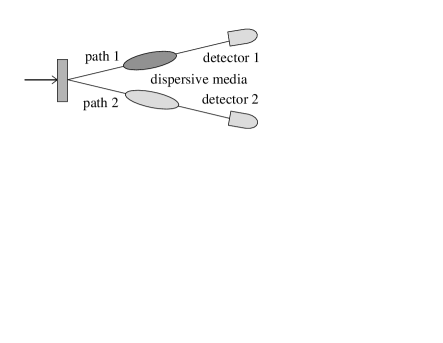
Figure 1: The source generates a state in which $N$ photons of frequency $\omega_{o}+\epsilon$ travel in path 1 towards detector 1, and $N$ photons $(\omega_{o}-\epsilon)$ travel in path 2 towards detector 2. The dispersive medium in path 1 is described by $\alpha_{1}$ and $\beta_{1}$, and similarly for path 2.

Including the dispersive properties of the two media, the amplitude $A$ of state $|A\rangle$ can be written as

$$\begin{split}A&=\frac{1}{N!}\int d\epsilon\,\phi(\omega_{o}+\epsilon)\exp[i\epsilon N(\alpha_{1}x-\alpha_{2}x^{\prime})]\\ &\times\exp[i\epsilon^{2}N(\beta_{1}x+\beta_{2}x^{\prime})]\exp[-i\epsilon N(\overline{t}-\overline{t}^{\prime})].\\ \end{split}$$ (7)

An overall phase factor has been dropped and we have defined the mean detection times $\overline{t}\equiv\frac{1}{N}\sum_{j=1}^{N}t_{j}$ and similarly $\overline{t}^{\prime}\equiv\frac{1}{N}\sum_{j=1}^{N}t_{j}^{\prime}$.

It can be seen from Eq. (7) that the effects of dispersion will cancel non-locally between the two media if $\beta_{1}x=-\beta_{2}x^{\prime}$, as was shown previously Franson (1992) for the case of $N=1$. The non-classical noise reduction inherent in Eq. (7) can be best understood by comparing these results with those from a single-photon wave packet with the same spectral function $\phi(\omega)$:

$$|\Psi_{1}\rangle=\int_{-\infty}^{\infty}\!d\epsilon\,\phi(\omega_{o}+\epsilon)\hat{a}^{\dagger}|0\rangle$$ (8)

If we define $g(t)$ as the Fourier transform of $\phi(\omega)$

$$g(t)=\int_{-\infty}^{\infty}\!\phi(\omega)e^{-i\omega t}\,d\omega$$ (9)

then $|g(t)|^{2}$ gives the intensity of the wave packet as a function of time at a fixed position ($x=0$). A similar result holds for classical pulses, and the width $\sigma_{g}$ of $|g(t)|^{2}$ is equal to the uncertainty in the timing information that can be obtained from a single photon wave packet with spectral function $\phi(\omega)$. If $N$ independent single-photon wave packets are transmitted, the timing uncertainty can be reduced to $\sigma_{g}/\sqrt{N}$, which corresponds to the classical shot noise limit. Comparison with Eq. (7) for the case in which $x=x^{\prime}$, $\alpha_{1}=\alpha_{2}$, and $\beta_{1}=-\beta_{2}$ shows that, for the entangled state $|\Psi\rangle$

$$|A(\tau)|^{2}=\frac{1}{N!^{2}}|g(N\tau)|^{2}.$$ (10)

Here $\tau$ is defined as the difference in mean arrival times, $\tau=\overline{t}-\overline{t}^{\prime}$. It can be seen from Eq. (10) that $|A|^{2}$ has a width that is a factor of $1/N$ less than that of the corresponding single-photon wave packet, which results in a factor of $1/\sqrt{N}$ reduction in the noise as compared to $N$ independent single-photon wave packets. Thus our results with dispersion cancellation are similar to those obtained from Eq. (2) by Giovannetti, Lloyd, and Maccone Giovannetti et al. (2001b), who did not include the effects of dispersion. The factor of $1/N$ improvement in timing resolution is closely related to the $1/N$ improvement in spatial resolution proposed by Boto et al. for use in quantum lithography Boto et al. (2000).

The above results show that nonlocal cancellation of dispersion and a non-classical reduction of noise can occur simultaneously for entangled states with large photon numbers. The condition $\beta_{1}x=-\beta_{2}x^{\prime}$ can be achieved in optical fibers Brendel et al. (1998), for example, but would be difficult to achieve under more general conditions, such as for the case of light beams propagating through the atmosphere. As a result, it is important to consider the effects of uncompensated dispersion on the non-classical noise reduction of states of this kind. All of the necessary integrals can be evaluated analytically for the case in which the spectral function $\phi(\omega_{o}+\epsilon)$ is assumed to be Gaussian with width $\sigma_{\phi}$

$$\phi(\omega_{o}+\epsilon)=\exp(-\epsilon^{2}/2\sigma_{\phi}^{2}).$$ (11)

For simplicity, we have omitted a normalization constant in Eq. (11). A Gaussian may, for example, represent a narrow bandwidth filter of the kind that is widely used in down-conversion experiments. For convenience, we will define $a_{\phi}^{2}\equiv(2\sigma_{\phi}^{2})^{-1}$, and obtain

$$A=\frac{1}{N!}\int_{-\infty}^{\infty}\!\!d\epsilon\,\exp\{-[\epsilon^{2}(a_{\phi}^{2}-iNB)+i\epsilon N\zeta]\}$$ (12)

where we have defined $B\equiv(\beta_{1}x+\beta_{2}x^{\prime})$ and $\zeta\equiv\tau-(\alpha_{1}x-\alpha_{2}x^{\prime})$. (Recall $\tau=\overline{t}-\overline{t}^{\prime}$.)

The integral may be evaluated by completing the square in the exponent, and aside from an overall phase factor

$$A=\frac{1}{N!}\frac{\sqrt{\pi}}{\sqrt{\smash[b]{a_{\phi}^{2}-iNB}}}\exp\left(\frac{-N^{2}\zeta^{2}}{4(a_{\phi}^{2}-iNB)}\right)$$ (13)

$$\langle A|A\rangle\!=\!|A|^{2}\!=\!\frac{\pi}{N!^{2}\sqrt{\smash[b]{a_{\phi}^{4}+N^{2}B^{2}}}}\exp\!\left(\frac{-(\tau-\overline{\tau})^{2}N^{2}a_{\phi}^{2}}{2(a_{\phi}^{4}+N^{2}B^{2})}\right)$$ (14)

where $\overline{\tau}=(\alpha_{1}x-\alpha_{2}x^{\prime})$. Equation (14) is thus a Gaussian in $\tau$ with mean $\overline{\tau}$ and width $\sigma_{\tau}$ given by

$$\sigma_{\tau}^{2}=\frac{a_{\phi}^{4}+N^{2}B^{2}}{N^{2}a_{\phi}^{2}}$$ (15)

$$\sigma_{\tau}^{2}=\frac{1+4\sigma_{\phi}^{4}N^{2}(\beta_{1}x+\beta_{2}x^{\prime})^{2}}{2\sigma_{\phi}^{2}N^{2}}$$ (16)

If the distances $x$ and $x^{\prime}$ are regarded as known, then $|A|^{2}$ describes a Gaussian probability distribution for the difference in mean arrival times. As we observed above, this allows dispersion cancellation Franson (1992) for $\beta_{1}x=-\beta_{2}x^{\prime}$, in which case $\sigma_{\tau}=1/(\sqrt{2}\sigma_{\phi}N)$.

However, if the dispersion cannot be cancelled or neglected, the scaling with large $N$ is independent of $N$:

$$\lim_{N\rightarrow\infty}\sigma_{\tau}=\sqrt{2}\sigma_{\phi}\left|\beta_{1}x+\beta_{2}x^{\prime}\right|$$ (17)

One might expect to approach the classical limit for large photon numbers and indeed in this case the quantum mechanical enhancement disappears. In fact, the timing uncertainty associated with the entangled state $|\Psi\rangle$ under these conditions is worse than the classical shot noise limit, since Eq. (17) does not include a factor of $1/\sqrt{N}$, as is the case classically. The transition point between these two limits occurs when

$$1=4\sigma_{\phi}^{4}N_{\mathrm{transition}}^{2}(\beta_{1}x+\beta_{2}x^{\prime})^{2}$$ (18)

At the transition point, $\sigma_{\tau}$ is $\sqrt{2}$ times the limiting value of Eq. (17), and further increases of $N$ above $N_{\mathrm{transition}}$ have diminishing effects. For typical optical materials such as fused silica, the group delay dispersion (at 800 nm) is $2\beta\sim 500\ \mathrm{fs}^{2}/\mathrm{cm}$ Walmsley et al. (2001). For a 5 nm bandwidth (one sigma) centered at 800 nm, $\sigma_{\phi}\sim 3.7\times 10^{11}$ rad/sec. A 1 cm thickness of fused silica in both paths would produce enough dispersion such that $N_{\mathrm{transition}}\sim 7.3\times 10^{3}$. Choosing a more modest $N_{\mathrm{transition}}=100$, the dispersion of 146 cm of fused silica in both paths is required. Similar remarks apply to the state vector of Eq. (2), which does not allow dispersion cancellation.

Non-classical noise reduction of this kind has been proposed Giovannetti et al. (2001b) for the synchronization of clocks on orbiting satellites. But in applications of that kind, the atmospheric dispersion cannot in general be cancelled or neglected with the exception of satellite-to-satellite links that do not pass through the atmosphere. We can estimate the dispersion of air using empirical relations for the index of refraction. Since $k_{\mathrm{air}}(\omega)=\frac{\omega}{c}n_{\mathrm{air}}(\omega)$ we have

$$\beta=\frac{1}{2}\,\frac{d^{2}k(\omega)}{d\omega^{2}}=\frac{1}{2c}\,\frac{d^{2}}{d\omega^{2}}\left(\omega\,n(\omega)\right)$$ (19)

The widely-used $n_{\mathrm{air}}$ formula of Edlén Edlén (1966) yields $\beta_{\mathrm{air}}=0.106$ fs²/cm at 800 nm for standard dry air at 15^∘C. Including 20% relative humidity using the more accurate formula of Owens Owens (1967) for $n_{\mathrm{air}}$ gives $\beta_{\mathrm{air}}=0.103$ fs²/cm at 800 nm. Thus $\sim$24 m of air has dispersion equivalent to 1 cm of fused silica, and long air path lengths would significantly limit the non-classical noise reduction suggested in Ref. Giovannetti et al. (2001b).

For a pair of classical Gaussian pulses, it was previously shown Franson (1992) that

$$|g(\tau)|^{2}=\exp(-(\tau-\tau_{o})^{2}/2\sigma_{T}^{2})$$ (20)

where $\tau_{o}=\alpha_{2}x_{2}-\alpha_{1}x_{1}$, and the width, in the notation used here, is

$$\sigma_{T}^{2}=\frac{2a_{\phi}^{4}+(\beta_{1}^{2}x_{1}^{2}+\beta_{2}^{2}x_{2}^{2})}{a_{\phi}^{2}}.$$ (21)

There is no possibility of dispersion cancellation in the classical case since Eq. (21) contains the sum of squares of the $\beta$ coefficients. In the limit of large dispersion, it can be seen that Eq. (21) is equivalent to the limiting case of Eq. (17), except that the overall timing uncertainty in Eq. (21) can be reduced by the square root of the number of photons in each path by classical averaging. This gives the classical timing uncertainty $\sigma_{\mathrm{C}}\equiv\sigma_{T}/\sqrt{N}$. In the quantum case, Eqs. (16) and (17) already represent the distribution of the average detection time, giving the quantum timing uncertainty $\sigma_{\mathrm{Q}}\equiv\sigma_{\tau}$. The quantum and classical expressions are plotted as a function of $N$ in Fig. 2 for a dispersive path of 4 m of fused silica (or 10 km of air), and a bandwidth $\sigma_{\phi}=3.7\times 10^{11}$ Hz centered at 800 nm. We plot $\sigma_{\phi}\sigma_{\mathrm{Q}}$, which is dimensionless, and similarly $\sigma_{\phi}\sigma_{\mathrm{C}}$ for the classical expression.

When the photon number or the dispersion is large, the quantum mechanical timing uncertainty is larger than the corresponding classical case, as shown in Fig. 3, where the ratio $\sigma_{\mathrm{Q}}/\sigma_{\mathrm{C}}$ is plotted as a function of photon number $N$ and distance $x$ (cm) in fused silica. To highlight the region where the quantum timing uncertainty is larger than the classical timing uncertainty, the plot has been clipped at unity and the clipped region rendered black.

Figure 2: A comparison of the classical (dashed line) and quantum (solid line) timing uncertainties. The widths $\sigma_{\mathrm{Q}}$ and $\sigma_{\mathrm{C}}$ have been multiplied by the spectral bandwidth $\sigma_{\phi}$ to give a dimensionless parameter $p$. Note that for a fixed dispersion, (in this case 4 m of fused silica or 10 km of air) the quantum mechanical expression rapidly approaches its asymptote, while the corresponding classical width decreases as $1/\sqrt{N}$ from classical averaging.

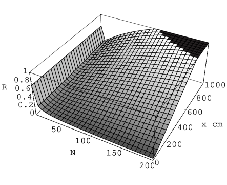
Figure 3: A surface plot of the ratio $R$ of the quantum mechanical width to the classical width, $\sigma_{\mathrm{Q}}/\sigma_{\mathrm{C}}$, as a function of $N$ and propagation distance $x$ (cm) through a dispersive medium with $\beta=250$ fs²/cm (fused silica) and a bandwidth $\sigma_{\phi}=3.7\times 10^{11}$ Hz. The quantum mechanical timing uncertainty is larger than the corresponding classical case in the black region in the upper right hand corner.

III Thick detectors

In the previous section, we considered the distance from the source to the detectors as fixed and found that the spread in arrival times had a narrow distribution. What if the roles of $x$ and $t$ are interchanged at the detector? Here we consider a gedanken experiment in which the detectors are thick in the $x$-direction, and can be activated (gated on) for a narrow time interval $\delta t$. During the time that it is gated on, the photons travelling inside a detector have some probability of being detected at positions that are registered. Such a detector might resemble a photographic emulsion that is activated by an ultrashort laser pulse, as depicted in Fig. 4. We now calculate the distribution of the detected positions.

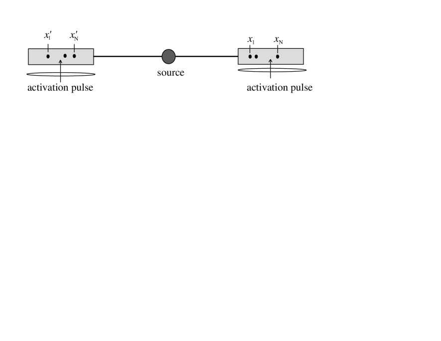
Figure 4: A thick, position-sensitive detector is assumed to be gated on for a narrow time interval $\delta t$ by a laser pulse. The positions of the detected photons, which are $\{x_{1}\cdots x_{N}\}$ for one side and $\{x_{1}^{\prime}\cdots x_{N}^{\prime}\}$ for the other, are recorded by the detectors.

Considering the same entangled state $|\Psi\rangle$ as before in Eqs. (1) and (3), we now consider the detection time in each arm fixed and ask what are the positions of the photons at the time of detection. Here we construct $A=A(x_{1}\cdots x_{N};x_{1}^{\prime}\cdots x_{N}^{\prime};t,t^{\prime},\delta t)$, where $|A|^{2}$ is proportional to the probability of detecting $N$ photons at positions $x_{1}\,,\cdots,\,x_{N}$ at detector 1 in time interval $(t_{1},t_{1}+\delta t)$ and $N$ photons at positions $x_{1}^{\prime}\,,\cdots,\,x_{N}^{\prime}$ at detector 2 in time interval $(t_{2},t_{2}+\delta t)$.

$$\begin{split}|A\rangle=\int_{t_{1}}^{t_{1}+\delta t}\!\!dt\int_{t_{2}}^{t_{2}+\delta t}\!\!dt^{\prime}&\hat{E}^{(+)}_{1}(x_{1},t)\cdots\hat{E}^{(+)}_{1}(x_{N},t)\\ \times&\hat{E}^{(+)}_{2}(x_{1}^{\prime},t^{\prime})\cdots\hat{E}^{(+)}_{2}(x_{N}^{\prime},t^{\prime})|\Psi\rangle\\ \end{split}$$ (22)

Making use of the expansion of the field operators in Eq. (5) and the commutator as before gives the probability amplitude A:

$$\begin{split}A&=\frac{1}{N!}\int\!dt\int\!dt^{\prime}\int d\epsilon\,\phi(\omega_{o}+\epsilon)\\ &\times\exp[i\left(k(\omega)x_{1}-\omega t\right)]\cdots\exp[i\left(k(\omega)x_{N}-\omega t\right)]\\ &\times\exp[i\left(k(\omega^{\prime})x_{1}^{\prime}-\omega^{\prime}t^{\prime}\right)]\cdots\exp[i\left(k(\omega^{\prime})x_{N}^{\prime}-\omega^{\prime}t^{\prime}\right)]\\ \end{split}$$ (23)

where again $\omega=\omega_{o}+\epsilon$ and $\omega^{\prime}=\omega_{o}-\epsilon$. We define $\overline{x}\equiv(1/N)\sum_{j=1}^{N}x_{j}$ and similarly $\overline{x}^{\prime}\equiv(1/N)\sum_{j=1}^{N}x_{j}^{\prime}$. Including the dispersive properties of the media gives:

$$\begin{split}A&=\frac{1}{N!}\int\!\!dt\int\!\!dt^{\prime}\int\!\!d\epsilon\,\phi(\omega_{o}+\epsilon)\\ &\times\exp i\epsilon N(\alpha_{1}\overline{x}-\alpha_{2}\overline{x}^{\prime})\exp i\epsilon^{2}N(\beta_{1}\overline{x}+\beta_{2}\overline{x}^{\prime})\\ &\times\exp(-i\omega_{o}N(t+t^{\prime}))\exp(-i\epsilon N(t-t^{\prime}))\\ \end{split}$$ (24)

where an overall phase factor has been omitted. This can be rearranged to give

$$\begin{split}A&=\frac{1}{N!}\int_{t_{1}}^{t_{1}+\delta t}\!\!\!dt\int_{t_{2}}^{t_{2}+\delta t}\!\!\!dt^{\prime}\exp[-i\omega_{o}N(t+t^{\prime})]\\ &\times\int\!d\epsilon\,\phi(\omega_{o}+\epsilon)\exp[i\epsilon N((\alpha_{1}\overline{x}-t)-(\alpha_{2}\overline{x}^{\prime}-t^{\prime}))]\\ &\times\exp[i\epsilon^{2}N(\beta_{1}\overline{x}+\beta_{2}\overline{x}^{\prime})].\\ \end{split}$$ (25)

Note that the quantity $(\alpha_{1}\overline{x}-t)$ corresponds to the group delay along path 1, and a similar factor appears for path 2.

In the limit $\delta t\ll 1/(N\omega_{o})$, the time integrations become trivial and the factor $\exp(-i\omega_{o}N(t+t^{\prime}))$ reduces to a constant phase shift. We define $\tau\equiv t-t^{\prime}$ and $\tau_{o}\equiv\alpha_{1}\overline{x}-\alpha_{2}\overline{x}^{\prime}$. Then Eq. (25) is proportional to:

$$A=\frac{1}{N!}\int\!\!d\epsilon\,\phi(\omega_{o}+\epsilon)e^{-i\epsilon N(\tau-\tau_{o})}e^{i\epsilon^{2}N(\beta_{1}\overline{x}+\beta_{2}\overline{x}^{\prime})}.$$ (26)

Assuming a Gaussian for $\phi(\omega_{o}+\epsilon)$ as in Eq. (11), we can complete the square in the exponent to obtain

$$A=\frac{1}{N!}\frac{\sqrt{\pi}}{\sqrt{\smash[b]{a_{\phi}^{2}-iNB}}}\exp\left(-\frac{N^{2}(\tau-\tau_{o})^{2}}{4(a_{\phi}^{2}-iNB)}\right)$$ (27)

$$|A|^{2}=\frac{1}{N!^{2}}\frac{\pi}{\sqrt{\smash[b]{a_{\phi}^{4}+N^{2}B^{2}}}}\exp\left(-\frac{(\tau-\tau_{o})^{2}N^{2}a_{\phi}^{2}}{2(a_{\phi}^{4}+N^{2}B^{2})}\right)$$ (28)

This has the same features as Eq. (14) and corresponds to a Gaussian in the variable $\tau=t-t^{\prime}$ with mean $\tau_{o}\equiv\alpha_{1}\overline{x}-\alpha_{2}\overline{x}^{\prime}$. The width is the same as in Eq. (15) and (16).

Equation (28) shows that a gated detector can exhibit dispersion cancellation and nonlocal noise reduction involving the average position of detection that is analogous to the average detection times from a more conventional detector. If $\alpha_{1}=\alpha_{2}$, then the mean positions will be very nearly equal if $t_{1}=t_{2}$. If the clocks are known to be synchronized, then any difference between the distances to the two detectors can be found. Similarly, if the distances to the detectors are known, then the synchronization of the clocks could be checked.

IV Correlated 2N-photon state

The entangled state $|\Psi\rangle$ of Eqs. (1) and (3) corresponds to two beams of light with anti-correlated frequencies, as is produced by parametric down-conversion for the case of $N=1$. In this section, we investigate the question of whether or not nonlocal cancellation of dispersion and non-classical noise reduction can occur for an entangled state with correlated frequencies instead, such as the state $|\Psi^{\prime}\rangle$ given by

$$|\Psi^{\prime}\rangle=\int d\epsilon\,\phi(\omega_{o}+\epsilon)\,|N(\omega_{o}+\epsilon)\rangle_{1}\,|N(\omega_{o}+\epsilon)\rangle_{2}$$ (29)

Newly proposed techniques for source engineering Branning et al. (1999); Erdmann et al. (2000); Banaszek et al. (2001) may be able to produce the state $|\Psi^{\prime}\rangle$ at least for small values of $N$. States with spectral correlation and anti-correlation were theoretically studied (for the case $N=1$) by Campos et al. Campos et al. (1990).

As above, the probability of detecting $N$ photons at times $\{t_{1},\cdots,t_{N}\}$ and positions $\{x_{1},\cdots,x_{N}\}$ in detector 1 and $N$ photons at times $\{t_{1}^{\prime},\cdots,t_{N}^{\prime}\}$ and positions $\{x_{1}^{\prime},\cdots,x_{N}^{\prime}\}$ in detector 2 is proportional to an amplitude $|A^{\prime}|^{2}$ given by

$$\begin{split}A^{\prime}&=\frac{1}{N!}\int d\epsilon\,\phi(\omega_{o}+\epsilon)\\ &\times\exp[i\left(k(\omega)x_{1}-\omega t_{1}\right)]\cdots\exp[i\left(k(\omega)x_{N}-\omega t_{N}\right)]\\ &\times\exp[i\left(k(\omega^{\prime})x_{1}^{\prime}-\omega^{\prime}t_{1}^{\prime}\right)]\cdots\exp[i\left(k(\omega^{\prime})x_{N}^{\prime}-\omega^{\prime}t_{N}^{\prime}\right)]\\ \end{split}$$ (30)

where here, $\omega=\omega^{\prime}=\omega_{o}+\epsilon$. Including the effects of a dispersive medium in paths 1 and 2 and collecting the terms gives:

$$\begin{split}A^{\prime}&=\frac{1}{N!}\!\int\!\!d\epsilon\,\phi(\omega_{o}+\epsilon)\exp[i\epsilon N(\alpha_{1}\overline{x}+\alpha_{2}\overline{x}^{\prime})]\\ &\times\exp[i\epsilon^{2}N(\beta_{1}\overline{x}+\beta_{2}\overline{x}^{\prime})]\exp[-i\epsilon N(\overline{t}+\overline{t}^{\prime})]\\ \end{split}$$ (31)

As before, we assume that $\phi(\omega_{o}+\epsilon)$ is a Gaussian, and for convenience, we define $B\equiv(\beta_{1}\overline{x}+\beta_{2}\overline{x}^{\prime})$ and $\xi\equiv(\overline{t}-\alpha_{1}\overline{x}+\overline{t}^{\prime}-\alpha_{2}\overline{x}^{\prime})$. Then Eq. (31) becomes:

$$A^{\prime}=\frac{1}{N!}\int_{-\infty}^{\infty}d\epsilon\exp\bigl{(}-[\epsilon^{2}(a_{\phi}^{2}-iNB)+i\epsilon N\xi]\bigr{)}.$$ (32)

This integral can be evaluated to give

$$A^{\prime}=\frac{1}{N!}\frac{\sqrt{\pi}}{\sqrt{\smash[b]{a_{\phi}^{2}-iNB}}}\exp\left(-\frac{N^{2}\xi^{2}}{4(a_{\phi}^{2}-iNB)}\right)$$ (33)

$$|A^{\prime}|^{2}=\frac{1}{N!^{2}}\frac{\pi}{\sqrt{\smash[b]{a_{\phi}^{4}+N^{2}B^{2}}}}\exp\left(-\frac{(\tau^{\prime}-\overline{\tau}^{\prime})^{2}N^{2}a_{\phi}^{2}}{2(a_{\phi}^{4}+N^{2}B^{2})}\right)$$ (34)

In going from Eq. (33) to Eq. (34) we have considered the distances in each arm to be fixed, so that $\overline{x}\rightarrow x$ and $\overline{x}^{\prime}\rightarrow x^{\prime}$. Then we let $\tau^{\prime}=\overline{t}+\overline{t}^{\prime}$, and then $\xi=\tau^{\prime}-\overline{\tau}^{\prime}$ where $\overline{\tau}^{\prime}=(\alpha_{1}x+\alpha_{2}x^{\prime})$. Clearly Eq. (34) is a Gaussian distribution in $\tau^{\prime}$ with mean $\overline{\tau}^{\prime}$ and variance

$$\sigma_{\tau^{\prime}}^{2}=\frac{a_{\phi}^{4}+N^{2}B^{2}}{N^{2}a_{\phi}^{2}}$$ (35)

$$\sigma_{\tau^{\prime}}^{2}=\frac{1+4\sigma_{\phi}^{4}N^{2}(\beta_{1}x+\beta_{2}x^{\prime})^{2}}{2\sigma_{\phi}^{2}N^{2}}.$$ (36)

Equation (36) is identical in form to Eqs. (15) and (16) which shows that dispersion cancellation can occur equally well for entangled states with either correlated or anti-correlated frequencies when $\beta_{1}x=-\beta_{2}x^{\prime}$. This is due to the fact that the dispersive effects are proportional to $\epsilon^{2}$, which is the same for correlated or anti-correlated frequencies. However, the group velocity terms depend on $\epsilon$ itself, with the result that $\tau^{\prime}$ involves the sum of the detection times rather than the difference. Thus the detection times are highly anti-correlated when the frequencies are correlated, whereas the detection times are correlated in the more usual case where the frequencies are anti-correlated. This result has different implications for clock synchronization than before because it is the sum of the mean arrival times at the two detectors which has a narrow spread.

In the case where dispersive effects can be neither cancelled nor neglected, Eq. (36) has a limiting value for large $N$ given by $\sigma_{\tau^{\prime}}\rightarrow\sqrt{2}\sigma_{\phi}|\beta_{1}x+\beta_{2}x^{\prime}|$ as before.

V Entangled Coherent States

We have considered so far only Fock states with definite photon number. In this section it is shown that similar results can be achieved for frequency-entangled coherent states. The generation and propagation of entangled coherent states has attracted some recent interest Howell and Yeazell (2000); Chizhov et al. (2001); Filip et al. (2001); Wang et al. (2001).

A coherent state of frequency $\omega$ is defined as:

$$|\mathit{v},\omega\rangle=\exp(-|\mathit{v}|^{2}/2)\sum_{n=0}^{\infty}\frac{\mathit{v}^{n}}{\sqrt{n!}}|n(\omega)\rangle.$$ (37)

where $\mathit{v}$ is an arbitrary complex parameter Glauber (1963). This can be expanded using creation operators as

$$|\mathit{v},\omega\rangle=\exp(-|\mathit{v}|^{2}/2)\sum_{n=0}^{\infty}\frac{\mathit{v}^{n}}{n!}\left(\hat{a}^{\dagger}(\omega)\right)^{n}|0\rangle.$$ (38)

A coherent state has the property not that

$$\hat{a}(\omega_{i})|\mathit{v},\omega_{j}\rangle=\mathit{v}\,|\mathit{v},\omega_{j}\rangle\,\delta_{ij}$$ (39)

which we will make use of below. It follows from Eq. (39) that the mean number of photons in the state is $\langle\mathit{v}|\hat{n}|\mathit{v}\rangle=\langle\mathit{v}|\hat{a}^{\dagger}\hat{a}|\mathit{v}\rangle=|\mathit{v}|^{2}$.

The original entangled state of Eq. (1) can be generalized to

$$|\Psi_{\mathrm{coh}}\rangle=\int d\epsilon\,\phi(\omega_{o}+\epsilon)\,|\mathit{v},(\omega_{o}+\epsilon)\rangle_{1}\,|\mathit{u},(\omega_{o}-\epsilon)\rangle_{2}$$ (40)

where $|\mathit{v}|$ need not equal $|\mathit{u}|$. As before, $\langle A|A\rangle$ is proportional to the probability of detecting $N$ photons at times $\{t_{1}\cdots t_{N}\}$ in detector 1 and $N$ photons at times $\{t_{1}^{\prime}\cdots t_{N}^{\prime}\}$ in detector 2, where now

$$\begin{split}|A(t_{1},\cdots,t_{N}\,&;\,t_{1}^{\prime},\cdots,t_{N}^{\prime})\rangle=\hat{E}^{(+)}_{1}(x,t_{1})\cdots\hat{E}^{(+)}_{1}(x,t_{N})\\ &\times\hat{E}^{(+)}_{2}(x^{\prime},t_{1}^{\prime})\cdots\hat{E}^{(+)}_{2}(x^{\prime},t_{N}^{\prime})|\Psi_{\mathrm{coh}}\rangle\\ \end{split}$$ (41)

Inserting the expansion of the electric field operator from Eq. (5) and making use of Eq. (39) we have:

$$\begin{split}|A\rangle=\!\int\!\!d\epsilon\,\phi(\omega_{o}\!+\epsilon)&\,\mathit{v}\exp[i(k_{1}(\omega_{o}\!+\epsilon)x\!-(\omega_{o}+\epsilon)t_{1})]\cdots\mathit{v}\exp[i(k_{1}(\omega_{o}\!+\epsilon)x\!-(\omega_{o}+\epsilon)t_{N})]\\ \times&\mathit{u}\exp[i(k_{2}(\omega_{o}\!-\epsilon)x^{\prime}\!-(\omega_{o}\!-\epsilon)t_{1}^{\prime})]\cdots\mathit{u}\exp[i(k_{2}(\omega_{o}\!-\epsilon)x^{\prime}\!-(\omega_{o}-\epsilon)t_{N}^{\prime})]\\ \times&|\mathit{v},(\omega_{o}\!+\epsilon)\rangle_{1}\,|\mathit{u},(\omega_{o}\!-\epsilon)\rangle_{2}\\ \end{split}$$ (42)

In computing $\langle A|A\rangle$ there arise inner products of the form $\langle\mathit{v}^{\prime},\omega_{i}|\mathit{v},\omega_{j}\rangle$, but it can be shown Mandel and Wolf (1995) that

$$\langle\mathit{v}^{\prime},\omega_{i}|\mathit{v},\omega_{j}\rangle=\exp[-|\mathit{v}^{\prime}-\mathit{v}|^{2}/2]\exp[(\mathit{v}^{\ast}\mathit{v}^{\prime}-\mathit{v}\mathit{v}^{\prime\ast})/2]\delta_{ij}.$$ (43)

Again, defining $\overline{t}=(1/N)\sum_{j=1}^{N}t_{j}$ and similarly for $\overline{t}^{\prime}$, we have:

$$|A|^{2}=|\mathit{v}|^{2N}|\mathit{u}|^{2N}\left|\int\!d\epsilon\,\phi(\omega_{o}+\epsilon)\,\exp[i\epsilon N(\alpha_{1}x-\alpha_{2}x^{\prime})+i\epsilon^{2}N(\beta_{1}x+\beta_{2}x^{\prime})-i\epsilon N(\overline{t}-\overline{t}^{\prime})]\right|^{2}$$ (44)

where we have used the dispersive properties of the media.

Equation (44) has the same form as Eq.(7) and gives the same results as does the original entangled Fock state of Eq. (1), aside from the overall magnitude of the detection probabilities. The distribution of arrival times is given by Eqs. (14) through (16). As a result, dispersion cancellation and non-classical noise reduction can occur just as well for the entangled coherent states of Eq. (40) as for entangled Fock states, which seems somewhat surprising. Equally surprising is the fact that the dispersion cancellation and noise reduction are independent of the relative magnitudes of $|\mathit{u}|$ and $|\mathit{v}|$, provided that equal numbers of photons are detected in both detectors, as was assumed above. These results are a direct consequence of the fact that coherent states are eigenstates of the annihilation operation, as indicated in Eq. (39).

VI Summary

We have generalized nonlocal cancellation of dispersion to entangled states containing large numbers of photons. The same entangled states were also shown to exhibit a factor of $1/\sqrt{N}$ reduction in noise below the classical shot noise limit for timing applications such as clock synchronization Jozsa et al. (2000); Giovannetti et al. (2001b); Chuang (2000); Burt et al. (2001); Jozsa et al. (2001); Yurtsever and Dowling (2000); Preskill (2000). Similar results were obtained for several different types of entangled states, including anti-correlated states, correlated states, and entangled coherent states. The fact that effects of this kind can occur for entangled coherent states shows that these non-classical correlations are a fundamental result of entanglement and are not limited to number states.

Our results also show that relatively small amounts of dispersion can essentially eliminate the factor of $1/\sqrt{N}$ reduction in noise for timing applications that was proposed by Giovannetti, Lloyd, and Maccone Giovannetti et al. (2001b). This could have a major impact on practical applications of these techniques for clock synchronization whenever the photons must pass through a dispersive medium, such as the Earth’s atmosphere. Dispersion cancellation can, in principle, be used to restore the $1/\sqrt{N}$ noise reduction, but the effects described here require that the coefficient of dispersion have the opposite sign in the two media. This may be the case in some potential applications, such as clock synchronization using optical fibers, where the frequencies of the two photons could be chosen to be on opposite sides of the point of minimum dispersion in the fiber Brendel et al. (1998). There is no obvious way to satisfy this condition in air, however, which may limit the use of these techniques to satellite-to-satellite links that do not pass through the Earth’s atmosphere. Other forms of dispersion cancellation Steinberg et al. (1992a, b); Giovannetti et al. (2001a) are not subject to this requirement and may be more useful for free-space clock synchronization, although they are more restricted with regard to the optical paths of the photons and in other respects.

Regardless of any potential practical applications, these results show that there is a close connection between non-classical noise reduction and nonlocal cancellation of dispersion, which we have generalized to states containing large numbers of photons.

References

• Franson (1992) J. D. Franson, Phys. Rev. A 45, 3126 (1992).
• Steinberg et al. (1992a) A. M. Steinberg, P. G. Kwiat, and R. Y. Chiao, Phys. Rev. Lett. 68, 2421 (1992a).
• Steinberg et al. (1992b) A. M. Steinberg, P. G. Kwiat, and R. Y. Chiao, Phys. Rev. A 45, 6659 (1992b).
• Giovannetti et al. (2001a) V. Giovannetti, S. Lloyd, L. Maccone, and F. N. C. Wong, Phys. Rev. Lett. 87, 117902 (2001a).
• Larchuk et al. (1995) T. S. Larchuk, M. C. Teich, and B. E. A. Saleh, Phys. Rev. A 52, 4145 (1995).
• Agarwal and Gupta (1994) G. S. Agarwal and S. D. Gupta, Phys. Rev. A 49, 3954 (1994).
• Jeffers and Barnett (1993) J. Jeffers and S. M. Barnett, Phys. Rev. A 47, 3291 (1993).
• Jozsa et al. (2000) R. Jozsa, D. S. Abrams, J. P. Dowling, and C. P. Williams, Phys. Rev. Lett. 85, 2010 (2000).
• Giovannetti et al. (2001b) V. Giovannetti, S. Lloyd, and L. Maccone, Nature 412, 417 (2001b).
• Chuang (2000) I. L. Chuang, Phys. Rev. Lett. 85, 2006 (2000).
• Burt et al. (2001) E. A. Burt, C. R. Ekstrom, and T. B. Swanson, Phys. Rev. Lett. 87, 129801 (2001), quant-ph/0007030.
• Jozsa et al. (2001) R. Jozsa, D. S. Abrams, J. P. Dowling, and C. P. Williams, Phys. Rev. Lett. 87, 129802 (2001).
• Yurtsever and Dowling (2000) U. Yurtsever and J. P. Dowling, A Lorentz-invariant look at quantum clock synchronization protocols based on distributed engtanglement (2000), eprint quant-ph/0010097.
• Preskill (2000) J. Preskill, Quantum clock synchronization and quantum error correction (2000), eprint quant-ph/0010098.
• Giovannetti et al. (2002) V. Giovannetti, S. Lloyd, and L. Maccone, Phys. Rev. A 65, 022309 (2002).
• (16) It would be more precise to use boundary conditions that are periodic in a length $L$, which gives discrete frequencies and a commutator of the form ${{[\hat{a}_{\ell}(\omega_{i})\,,\,\hat{a}_{k}^{\dagger}(\omega_{j})]=\delta_{\ell k}\,\delta_{ij}}}$. After using the commutation relations, the remaining sums would reduce to the integrals shown in the text in the limit of large $L$, as usual.
• Weinfurter and Żukowski (2001) H. Weinfurter and M. Żukowski, Phys. Rev. A 64, 010102(R) (2001).
• Pan et al. (2001) J.-W. Pan, M. Daniell, S. Gasparoni, G. Weihs, and A. Zeilinger, Phys. Rev. Lett. 86, 4435 (2001).
• Ou et al. (1999) Z. Y. Ou, J.-K. Rhee, and L. J. Wang, Phys. Rev. Lett. 83, 959 (1999).
• Lee et al. (2001) H. Lee, P. Kok, N. J. Cerf, and J. P. Dowling, Linear optics and projective measurements alone suffice to create large-photon-number path entanglement (2001), eprint quant-ph/0109080.
• Kok et al. (2001) P. Kok, H. Lee, and J. P. Dowling, The creation of large photon-number path entanglement conditioned on photodetection (2001), eprint quant-ph/0112002.
• Fiurášek (2001) J. Fiurášek, Conditional generation of n-photon entangled states of light (2001), eprint quant-ph/0110138.
• Lamas-Linares et al. (2001) A. Lamas-Linares, J. C. Howell, and D. Bouwmeester, Nature 412, 887 (2001).
• Boto et al. (2000) A. N. Boto, P. Kok, D. S. Abrams, S. L. Braunstein, C. P. Williams, and J. P. Dowling, Phys. Rev. Lett. 85, 2733 (2000).
• Brendel et al. (1998) J. Brendel, H. Zbinden, and N. Gisin, Opt. Commun. 151, 35 (1998).
• Walmsley et al. (2001) I. Walmsley, L. Waxer, and C. Dorrer, Rev. Sci. Instr. 72, 1 (2001).
• Edlén (1966) B. Edlén, Metrologia 2, 71 (1966).
• Owens (1967) J. C. Owens, Appl. Opt. 6, 51 (1967).
• Branning et al. (1999) D. Branning, W. P. Grice, R. Erdmann, and I. A. Walmsley, Phys. Rev. Lett. 83, 955 (1999).
• Erdmann et al. (2000) R. Erdmann, D. Branning, W. Grice, and I. A. Walmsley, Phys. Rev. A 62, 053810 (2000).
• Banaszek et al. (2001) K. Banaszek, A. B. U’Ren, and I. A. Walmsley, Opt. Lett. 26, 1367 (2001).
• Campos et al. (1990) R. A. Campos, B. E. A. Saleh, and M. C. Teich, Phys. Rev. A 42, 4127 (1990).
• Howell and Yeazell (2000) J. C. Howell and J. A. Yeazell, Phys. Rev. A 62, 012102 (2000).
• Chizhov et al. (2001) A. V. Chizhov, E. Schmidt, L. Knöll, and D.-G. Welsch, J. Opt. B: Quantum Semiclass. Opt. 3, 77 (2001).
• Filip et al. (2001) R. Filip, J. Řeháček, and M. Dušek, J. Opt. B: Quantum Semiclass. Opt. 3, 341 (2001).
• Wang et al. (2001) L. J. Wang, C. K. Hong, and S. R. Friberg, J. Opt. B: Quantum Semiclass. Opt. 3, 346 (2001).
• Glauber (1963) R. J. Glauber, Phys. Rev. 131, 2766 (1963).
• Mandel and Wolf (1995) L. Mandel and E. Wolf, Optical coherence and quantum optics (Cambridge University Press, Cambridge, England, 1995).