Minimum-error discrimination between three mirror-symmetric states

Abstract

We present the optimal measurement strategy for distinguishing between three quantum states exhibiting a mirror symmetry. The three states live in a two-dimensional Hilbert space, and are thus overcomplete. By mirror symmetry we understand that the tranformation $\{|+\rangle\rightarrow|+\rangle,|-\rangle\rightarrow-|-\rangle\}$ leaves the set of states invariant. The obtained measurement strategy minimises the error probability. An experimental realization for polarized photons, realizable with current technology, is suggested.

Quantum communication theory is concerned with the transmission of information using quantum states and channels. A sender encodes a message onto a set of signal states, and the task for the receiving party is to decode the message as well as possible. Suppose $|\psi_{i}\rangle$ is a set of $M$ quantum states, each occurring with probability $p_{i}$. This set, the “letters of the alphabet”, and the prior probabilities are known also to the receiving party.

A general measurement strategy can be described in terms of a probability operator measure (POM), also called a probability operator-valued measure [1, 2, 3]. The different measurement outcomes, labeled by $j$, are associated with operators $\hat{\pi}_{j}$, called the elements of the POM. Given that the system to be measured is prepared in state $|\psi_{i}\rangle$, the probability to obtain result $j$ is

$$p(j|i)=\langle\psi_{i}|\hat{\pi}_{j}|\psi_{i}\rangle.$$ (1)

For a von Neumann measurement, the operators $\hat{\pi}_{j}$ are projectors onto the orthonormal eigenstates of the observable to be measured. In general, however, $\hat{\pi}_{j}$ are not orthogonal. Nevertheless, all the eigenvalues of $\hat{\pi}_{j}$ have to be positive or zero, and the POM elements sum to the identity operator, $\sum_{j}\hat{\pi}_{j}=\hat{\bf 1}$. These conditions reflect the facts that probabilities are non-negative and that the measurement always yields a result, even if the result might not provide any information.

The task is now to find an optimal measurement strategy based on the knowledge of the signal states and their prior probabilities. One possibility is to choose the measurement strategy which minimises the probability of error in assigning the correct signal state. If the prior probability for signal state $|\psi_{i}\rangle$ is $p_{i}$, the error probability is given by

$$P_{error}=1-\sum_{j=1}^{M}\langle\psi_{j}|\hat{\pi}_{j}|\psi_{j}\rangle p_{j}.$$ (2)

The conditions which the minimum-error strategy must satisfy are known to be[1]

$$\hat{\pi}_{j}(p_{j}|\psi_{j}\rangle\langle\psi_{j}|-p_{k}|\psi_{k}\rangle\langle\psi_{k}|)\hat{\pi}_{k} = 0\quad\forall\quad j,k,$$ (3)

$$\sum_{j=1}^{M}p_{j}|\psi_{j}\rangle\langle\psi_{j}|\hat{\pi}_{j}-p_{k}|\psi_{k}\rangle\langle\psi_{k}| \geq 0\quad\forall\quad k,$$ (4)

where the inequality in the second condition states that all the eigenvalues of the operator on the left-hand side must be greater than or equal to zero. These conditions are in general not transparent enough to be used for obtaining the optimal solution. In fact, the optimal strategy is only known for some special cases, including the case with only two signal states [1], symmetric states [1, 4, 5], and equiprobable states that are complete in the sense that a weighted sum of projectors onto the states equals the identity operator [6]. For linearly independent states, the optimal measurement is known in some cases [7].

We will consider the situation in which the signal states are given by

$$|\psi_{1}\rangle = \cos\theta|+\rangle+\sin\theta|-\rangle$$ (5)

$$|\psi_{2}\rangle = \cos\theta|+\rangle-\sin\theta|-\rangle$$ (6)

$$|\psi_{3}\rangle = |+\rangle,$$ (7)

with prior probabilitites $p_{1,2}=p$ and $p_{3}=1-2p$, where $0\leq p\leq 1/2$. Due to symmetry it is enough to consider the range $0\leq\theta\leq\pi/2$. The states $|+\rangle$ and $|-\rangle$ are orthonormal basis states. As a special case, the so-called trine states are obtained when $\theta=\pi/3$ and all the probabilities are equal to $1/3$ [8].

The transformation $\{|+\rangle\rightarrow|+\rangle,|-\rangle\rightarrow-|-\rangle\}$ leaves the set of signal states unchanged. We expect that the POM elements will exhibit the same symmetry as the set of signal states, and are led to the Ansatz

$$\hat{\pi}_{1,2} = |\phi_{1,2}\rangle\langle\phi_{1,2}|,$$ (8)

$$\hat{\pi}_{3} = (1-a^{2})|+\rangle\langle+|=|\phi_{3}\rangle\langle\phi_{3}|,$$ (9)

where

$$|\phi_{1,2}\rangle=1/\sqrt{2}(a|+\rangle\pm|-\rangle),$$ (10)

with “+” referring to $|\phi_{1}\rangle$, “-” to $|\phi_{2}\rangle$, and $0\leq a\leq 1$.

If $p$ is large enough (certainly if $p=1/2$), we might expect that the optimal measurement strategy is the one which distinguishes optimally between $|\psi_{1}\rangle$ and $|\psi_{2}\rangle$. This is the case when $a=1$ and

$$\hat{\pi}_{1} = {1\over 2}(|+\rangle+|-\rangle)(\langle+|+\langle-|),$$ (11)

$$\hat{\pi}_{2} = {1\over 2}(|+\rangle-|-\rangle)(\langle+|-\langle-|),$$ (12)

$$\hat{\pi}_{3} = 0.$$ (13)

It is convenient to start by investigating when this strategy is optimal. The POM elements (11) can be checked to satisfy condition (3). The inequality condition (4) is seen to hold for $k=1,2$. For $k=3$, using matrix notation,

$$|+\rangle\equiv\left(\begin{array}[]{c}1\\ 0\end{array}\right);|-\rangle\equiv\left(\begin{array}[]{c}0\\ 1\end{array}\right),$$ (14)

it can be written

$$p(\cos\theta+\sin\theta)\left(\begin{array}[]{c c}\cos\theta&0\\ 0&\sin\theta\end{array}\right)-(1-2p)\left(\begin{array}[]{c c}1&0\\ 0&0\end{array}\right)\geq 0,$$ (15)

which is satisfied if

$$p\geq{1\over{2+\cos\theta(\cos\theta+\sin\theta)}}.$$ (16)

Hence the measurement strategy given by Eq. (11), which distinguishes optimally between $|\psi_{1}\rangle$ and $|\psi_{2}\rangle$, is the best choice provided $p_{1,2}=p$ is large enough.

If $p$ is too small to satisfy the inequality (16), we need to consider a three-element POM, as given by the original Ansatz in Eq. (8). The equality condition (3) holds trivially for $j=1$ and $k=2$. For $j=1,2$ and $k=3$ it leads to the requirement

$$a={{p\cos\theta\sin\theta}\over{1-p(2+\cos^{2}\theta)}}.$$ (17)

With this value of $a$, the inequality condition (4) for $k=3$ is satisfied, the smaller eigenvalue being zero. To test the inequality condition for $k=1,2$, it is convenient to make use of the fact that a $2\times 2$ Hermitian matrix with elements $a_{11},a_{12},a_{21}$ and $a_{22}$ is positive semidefinite if and only if $a_{11},a_{22}$ and the determinant of the matrix are all greater that or equal to zero. Upon evaluating the l.h.s. of condition (4) in matrix form, one finds that its elements $a_{11}$, $a_{22}$ are both greater than zero. The determinant turns out to be zero when the required value of $a$ is used.

It follows that this is indeed the measurement strategy which minimises the error probability. As shown in Fig. 1, there are two regimes depending on $p$ and $\theta$. If $p_{1,2}=p$ is large enough to satisfy the inequality (16), the strategy with $\hat{\pi}_{3}=0$, which distinguishes optimally between $|\psi_{1}\rangle$ and $|\psi_{2}\rangle$, is the solution. If $p$ is smaller than this, the full three-element measurement is needed, with $a$ given by Eq. (17). The crossover between these two regimes corresponds to $p=(2+\cos\theta(\cos\theta+\sin\theta))^{-1}$, where the two strategies will coincide.

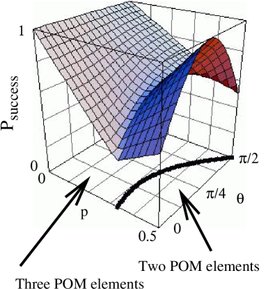
FIG. 1.: The success probability $P_{success}$ as a function of $p$ and $\theta$. The optimal measurement strategy will have either two or three elements.

It is straightforward to calculate the success probability, that is, the probability of correctly identifying the signal state, of the devised optimal measurement strategy. For $p\geq 1/\left[2+\cos\theta(\cos\theta+\sin\theta)\right]$, we find

$$P_{success}=1-P_{error}=p(1+\sin 2\theta).$$ (18)

As a special case, for $p=1/2$ with $0\leq\theta\leq\pi/2$, this reduces to the probability to distinguish with minimal error between two non-orthogonal states. For $p=1/2$ and $\theta=\pi/4$, the success probability is equal to one, corresponding to the situation where the two states are orthogonal.

For $p\leq 1/\left[2+\cos\theta(\cos\theta+\sin\theta)\right]$, the success probability is

$$P_{success}={{(1-2p)\left[p\sin^{2}\theta+1-2p-p\cos^{2}\theta\right]}\over{1-2p-p\cos^{2}\theta}},$$ (19)

which reduces to 2/3 for equal probabilities $(p_{1,2}=p_{3}=1/3)$, as long as $\pi/4\leq\theta\leq\pi/2$.

In many of the measurement situations where the optimal measurement strategy is known, the optimal strategy is the square-root or “pretty good” measurement [4, 7, 9] with POM elements

$$\pi_{i}=\hat{\rho}^{-1/2}p_{i}|\Psi_{i}\rangle\langle\Psi_{i}|\hat{\rho}^{-1/2},$$ (20)

where

$$\hat{\rho}=\sum_{i=1}^{3}p_{i}|\Psi_{i}\rangle\langle\Psi_{i}|.$$ (21)

It is interesting to note that the square root measurement strategy will coincide with the optimal strategy for some nontrivial $p$ and $\theta$, but is in general not the optimal strategy.

In a way similar to recent optical realisations of generalised measurements [8, 10, 11, 12], it is possible to realise the devised measurement strategy for photon polarization. The states $|+\rangle$ and $|-\rangle$ will now correspond to orthogonal polarisation states of a single photon, for example horizontal and vertical linear polarisation $|H\rangle$ and $|V\rangle$. The realisation relies on the fact that any generalised measurement can be extended to a projective (von Neumann) measurement in a higher-dimensional Hilbert space, the so-called Naimark extension [1, 2, 3, 13]. Physically, this can be achieved by coupling the system to an ancilla, or for example as in the optical realisations, by the introduction of additional input ports to the system, thus extending the Hilbert space.

An optical network with beam splitters and wave plates can be used to couple the different polarisation states, and the measurement result is obtained by detecting where the photon exits, as shown in Fig. 2. The signal state is incident on one of the input ports of the polarising beam splitter PBS1. In the case we are considering, one auxiliary degree of freedom is needed, and this is provided by the second input port of the beam splitter. Only vacuum is incident through this input.

FIG. 2.: Optical network for implementing the minimum-error measurement on the three mirror-symmetric states. The state to be measured is incident on PBS1. PBS1, PBS2 and PBS3 are polarising beam splitters, transmitting horisontally polarised light and reflecting vertically polarised light. WP1 and WP2 are waveplates, and M1 and M2 are mirrors.

In matrix notation, for correct settings of the waveplates [14], the optical network effects the unitary transformation

$$U={1\over\sqrt{2}}\left(\begin{array}[]{c c c}a&1&\sqrt{1-a^{2}}\\ a&-1&\sqrt{1-a^{2}}\\ \sqrt{2(1-a^{2})}&0&-\sqrt{2}a\end{array}\right),$$ (22)

using

$$|H\rangle_{1}\equiv\left(\begin{array}[]{c}1\\ 0\\ 0\end{array}\right),|V\rangle_{1}\equiv\left(\begin{array}[]{c}0\\ 1\\ 0\end{array}\right),|V\rangle_{2}\equiv\left(\begin{array}[]{c}0\\ 0\\ 1\end{array}\right).$$ (23)

Here $|H\rangle_{1}$ and $|V\rangle_{1}$ are used to encode the signal state, $|V\rangle_{2}$ being an auxiliary degree of freedom provided by the second input port of PBS1. The mode $|H\rangle_{2}$ is not coupled to the signal state modes, as horizontally polarized light incident through the second input port of PBS1 will be transmitted by both beam splitters, always resulting in detection at PD3. The rows of the matrix $U$ are simply the POM element vectors $|\phi_{1,2,3}\rangle$, but extended in the third auxiliary dimension so that the matrix row vectors are orthogonal.

The measurement at the output then distinguishes between horisontally and vertically polarised photons in mode 1 (PD1 and PD2, outcome 1 and 2), and (vertically polarised) photons in mode 2 (PD3, outcome 3). If the incident state is $|\psi_{i}\rangle$, the state after the network is

$$U|\psi_{i}\rangle=\sum_{j=1}^{3}|j\rangle\langle\phi_{j}|\psi_{i}\rangle,$$ (24)

where $|1\rangle\equiv|H\rangle_{1}$, $|2\rangle\equiv|V\rangle_{1}$ and $|3\rangle\equiv|V\rangle_{2}$. It is easy to confirm that

$$p(j|i) = \langle\psi_{i}|\hat{\pi}_{j}|\psi_{i}\rangle$$ (25)

$$= \langle j|U|\psi_{i}\rangle\langle\psi_{j}|U^{\dagger}|j\rangle,$$ (26)

so that the setup indeed realises the intended measurement strategy.

We want to stress that an optical setup like this is straightforward to realise. Indeed, a slightly different, but essentially equivalent network was used in the experiments of Clarke et al. [8, 12]. Another equivalent network was suggested, for a different measurement task, by Sasaki et al. [15], and has recently been realized experimentally [16]. In summary, we have obtained the measurement strategy which minimises the error probability when distinguishing between three mirror-symmetric states. This example is noteworthy in that the number of non-zero POM elements, for the minimum-error strategy, depends on the parameters chosen for the set of states. It will be interesting to see if this unusual property persists for other measures of detection strategy such as mutual information [15] and fidelity [17].

We would like to thank P. Öhberg for his assistance in preparing the manuscript. This work was supported by the European Commission Marie Curie Fellowship scheme, the Royal Society of Edinburgh, the Scottish Executive Education and Lifelong Learning Department, the International Centre for Theoretical Physics and the UK Engineering and Physical Sciences Research Council.

REFERENCES

- [1] C. W. Helstrom, Quantum detection and estimation theory (Academic, New York, 1976).
- [2] K. Kraus, States, Effects and Operations: Fundamental Notions of Quantum Theory (Springer, Berlin, 1983).
- [3] A. Peres, Quantum Theory: Concepts and Methods, (Kluwer Academic Publishers, Dordrecht 1993).
- [4] M. Ban, Y. Kamazaki, R. Momose, and O. Hirota, Int. J. Theor. Phys. 36, 1269 (1997).
- [5] S. M. Barnett, Phys. Rev. A 64, 030303(R) (2001).
- [6] H. P. Yuen, R. S. Kennedy, and M. Lax, IEEE Trans. Inf. Theory IT-21, 125 (1975).
- [7] M. Sasaki, K. Kato, M. Izutsu, and O. Hirota, Phys. Rev. A 58, 146 (1998).
- [8] R. B. M. Clarke, V.M. Kendon, A. Chefles, S. M. Barnett, E. Riis, and M. Sasaki, Phys. Rev. A 64, 012303 (2001).
- [9] P. Hausladen and W. K. Wootters, J. Mod. Opt. 41, 2385 (1994).
- [10] B. Huttner, A. Müller, J. D. Gautier, H. Zbinden, and N. Gisin, Phys. Rev. A 54, 3783 (1996).
- [11] S. M. Barnett and E. Riis, J. Mod. Opt. 44, 1061 (1997).
- [12] R. B. M. Clarke, A. Chefles, S. M. Barnett, and E. Riis, Phys. Rev. A 63, 040305 (2001).
- [13] M. A. Neumark, Izv, Akad. Nauk. SSSR, Ser. Mat. 4, 227 (1940).
- [14] The wave plates rotate the polarisation according to with and , where .
- [15] M. Sasaki, S. M. Barnett, R. Jozsa, M. Osaki, and O. Hirota, Phys. Rev. A 59, 3325 (1999).
- [16] J. Mizuno, M. Fujiwara, M. Sasaki, M. Akiba, T. Kawanishi, and S. M. Barnett, Phys. Rev. A. 65, 012315 (2002).
- [17] S. M. Barnett, C. R. Gilson, and M. Sasaki, J. Phys. A: Math. Gen. 34, 6755 (2001); C. Fuchs and M. Sasaki (private communication).