Sensitivity to Initial Conditions in Quantum Dynamics: an Analytical Semiclassical Expansion

Abstract

We construct a class of systems for which quantum dynamics can be expanded around a mean field approximation with essentially classical content. The modulus of the quantum overlap of mean field states naturally introduces a classical distance between classical phase points. Using this fact we analytically show that the time rate of change (trc) of two neighbouring classical trajectories is directly proportional to the trc of quantum correlations. Coherence loss and nonlocality effects appear as corrections to mean field dynamics and we show that they can be given in terms of classical trajectories and generalized actions. This result is a first step in the connection between quantum and classically chaotic dynamics in the same sense of semiclassical expansions for the density of states. We apply the results to the nonintegrable (classically chaotic) version of the N-atom Jaynes-Cummings model.

Ever since the conception of Quantum Mechanics the classical limit has been a matter of much debate due to the profound contrasting differences between the classical and quantal descriptions of the world. Although the difficulties in building a bridge between quantum and classical mechanics are well known, we start by reviewing the ones which are of relevance for the present contribution. As far as kinematical differences are concerned, already at the level of a point particle, striking differences appear. While the definition of the state of a classical particle is of local character and given by a point in phase space, the quantum counterpart of the definition of a particle state is given by a vector in Hilbert space which cannot simultaneously be ascribed a well defined value for position and momentum. The closer one can get to the classical situation are minimum uncertainty wave packets. Quantum states are therefore usually nonlocal. Also, the linear character of the Hilbert space has the immediate consequence that superposition of (minimum uncertainty) states are also possible states and, in fact, constitute the vast majority of allowed quantum states. The situation gets even cloudier when two degrees of freedom are involved: Classically one can always describe a two particle state in terms of the coordinates and momenta of each one of them. Quantum mechanically, however, this situation only holds if the two particles, initially in a factorized state, do not interact. The Hilbert space structure allows for states which cannot be written as a direct product of vectors in the individual Hilbert spaces of each degree of freedom. This essentially quantum property is usually named entanglement. Much investigation and progress both on the theoretical and experimental sides have been achieved recently. [1]

From the dynamical point of view one of the essential differences has given rise to an important research area nowadays: classical chaos, a phenomenon whose root lies on the nonlinearity of Newton’s equation. The relevant question here is how to identify the quantum counterpart of classical chaos. A major step in this direction was given by Bohigas and collaborators who conjectured that spectral properties of integrable and nonintegrable systems should be very different [2]. Thereafter many numerical investigations confirmed such conjecture and a few exceptions where found. From the analytical point of view a most relevant formula was derived by Gutzwiller connecting level densities of very general quantum systems with classical periodic orbits and their actions[3]. In what concerns the connections between classical and quantum dynamics it has recently been proposed by Zurek that the rate of entropy production can be used as an intrinsically quantum test of the chaotic vs. regular nature of the evolution[4]. Several numerical tests of this conjecture can also be found[5, 6]. Anyway, analytic results in this context are scarce. This letter is a step in the direction of filling in this gap.

Given the considerations above we restrict ourselves to the study of the (two degrees of freedom) hermitian bilinear hamiltonians

$$H=\sum_{i}\alpha_{i}A_{i}+\sum_{j}\beta_{j}B_{j}+\sum_{i,j}\gamma_{i,j}A_{i}B_{j},$$ (1)

where $i,j={0,\pm}$, A and B are chosen among the generators of either the $h(3)$ (Heisenberg group) or $SU(2)$ groups. Index 0 is associated with the operator $a^{\dagger}a$ ($J_{z}$), the index $+$ with the operator $a^{\dagger}$ ($J_{+}$) and the index $-$ with the operator $a$ ($J_{-}$) for the algebra $h(3)$ ($su(2)$). The coefficients $\alpha$, $\beta$ and $\gamma$ are constants or given functions of time.

Although seemingly trivial this class of systems encompasses a rich variety of dynamical behavior including the model we shall use for illustration whose clasical limit is chaotic. The choice of the groups $h(3)$ and $SU(2)$ is due to the fact that several of the problems mentioned above can be circumvented at the lowest order, the mean field. Due to the bilinear character of the hamiltonian, a time dependent mean field solution will be products of coherent states whose labels satisfy the classical limit of Heinsenberg’s equations of motion as can be easily verified. No quantum dynamical nonlocality effects appear at this level (lowest order) unlike mean field approximations for other systems. All quantum corrections will appear in next to leading orders as we will show.

The zeroth order approximation: The mean field approximation (MFA) and the classical limit.

Our zeroth order approximation is defined in the following way:

a) We consider here states of the form of products of coherent states and a phase

$$|\psi(t)\rangle=\exp(i\eta(t))|x(t)\rangle\otimes|y(t)\rangle,$$ (2)

where the minimum uncertainty coherentes states $|z(t)\rangle$ are defined by $|z(t)\rangle={\cal D}(z(t))|0\rangle$ with

$${\cal D}(z(t))=\left\{\begin{array}[]{l}\exp[z(t)a^{\dagger}-z^{*}(t)a]\\ \exp[\frac{\operatorname{atan}|z(t)|}{|z(t)|}(z(t)J_{+}-z^{*}(t)J_{-})],\end{array}\right.$$ (3)

for h(3) and su(2) respectively, and the fiducial state $|0\rangle$ is the Fock state $|n=0\rangle$ for h(3) and the $J_{z}$ eigenstate $|J,-J\rangle$ for su(2).

b) Linear combinations are not allowed as initial conditions (this circumvents problems with the superposition principle). Also this MFA for the systems (1) will leave invariant the manifold of the chosen set of trial functions.

At this point it is important to mention that the algebra h(3) could be easily enlarge to include of harmonic oscillator algebra with little effort, but the extra terms give rise to nonlocality effects (squeezing dynamics) already at this lowest order which we would like to avoid. Notice also that generalization to n degrees of freedom m-linear hamiltonians ($m\leq n$) is straightforward.

Now we solve the mean field Schrödinger equation

$$(i\partial_{t}-\bar{H})|\psi(t)\rangle,$$ (4)

where $\hbar=1$ and the mean field hamiltonian (MFH) is

$$\bar{H}=1_{A}\otimes H_{B}(x(t))+H_{A}(y(t))\otimes 1_{B},$$

with $H_{B}(x(t))=\langle x(t)|H|x(t)\rangle$. Using the explicit form of the hamiltonian (1) we find

$$H_{A}(t)=\sum_{i}a_{i}(t)A_{i}+f_{A}(t),$$ (5)

where $a_{i}(t)=\alpha_{i}+\sum_{j}\gamma_{ij}\langle y|B_{j}|y\rangle$ and $f_{A}(t)=\sum_{j}\beta_{j}\langle y|B_{j}|y\rangle$. The expression for $H_{B}(t)$ is completely analogous to the expression for $H_{A}(t)$. Since the terms $f_{A}(t)$, $f_{B}(t)$ give rise to global phases we neglect them. Due to the structure of the MFH the solutions of eq. (4) will preserve the form (2), and their time dependence will be completely specified by the solutions of the following equations of motion

$$\dot{z} = -ia_{0}z-ia_{+}\hskip 79.6678pt(\mbox{h(3)})$$ (6)

$$\dot{z} = -ia_{+}-ia_{0}z+i(a_{+})^{*}z^{2}\hskip 28.45274pt(\mbox{su(2)})$$ (7)

$$\dot{\eta}_{z} = \langle 0|{\cal D}^{\dagger}(z(t))\left(i\partial_{t}-h(t)\right){\cal D}(z(t))|0\rangle.$$ (8)

Observe that the total phase $\eta(t)$ is the sum of the partial phases $\eta_{x}(t)$ and $\eta_{y}(t)$. The nonlinearity of these equations arise from the self consistency of MFA. If the labels are scaled as $z=\sqrt{4J}Z$ for h(3), $z=Z$ for su(2), and time as $t=t_{c}/(4J)$, then the equations for $Z(t_{c})$ will become independent of $J$ and correspond to the classical limit of Heisenberg’s equations of motion. From equation (8) it follows that the phases $\eta_{z}(t)$ are generalized actions of the coherent state $|z(t)\rangle$. They are of course absent from the classical limit, but will be crucial for the quantum corrections.

Thus, we have shown that systems with hamiltonian (1), in the mean field approximation satisfy all the requirements we wanted: labels with classical physical meaning, no superposition principle, minimum quantum nonlocality effects, and hamiltonian equations for labels which coincide with both the exact Schrödinger equation and the Heisenberg equations of motion.

Quantum corrections.

Now we turn to the corrections to the MFA. The exact Schrödinger equation for the whole system (with the tilde indicating the Schrödinger picture)

$$i\partial_{t}\tilde{|\psi(t)\rangle}=(\bar{H}(t)+\tilde{\Delta}(t))\tilde{|\psi(t)\rangle},$$

where $\tilde{\Delta}(t)=H-\bar{H}(t)$, can be written in the MFA interaction picture (MFAIP) as (the absence of the tilde indicating the MFAIP)

$$i\partial_{t}|\psi(t)\rangle=\Delta(t)|\psi(t)\rangle=\sum_{ij}\gamma_{ij}(A_{i}(t)-\langle A_{i}\rangle(t))(B_{j}(t)-\langle B_{j}\rangle(t))|\psi(t)\rangle,$$ (9)

again up to time dependent terms that give rise to a global phase. Here we have defined $A(t)$ and $\langle A\rangle(t)$ as

$$\begin{split}A(t)&=\bar{U}^{\dagger}(t,0)A\bar{U}(t,0),\\ \langle A\rangle(t)&=\langle 0|{\cal D}^{\dagger}(x(t))A{\cal D}(x(t))|0\rangle,\end{split}$$

where $\bar{U}(t,0)$ is the evolution operator of the MFA, the product of the evolution operators for each degree of freedom. The equations for $B(t)$ and $\langle B\rangle(t)$ are completely analogous. Equation (9) possesses a natural expansion

$$|\psi_{t}\rangle=(1-i\int_{0}^{t}dt_{1}\Delta_{t_{1}}-\int_{0}^{t}dt_{1}\int_{0}^{t_{1}}dt_{2}\Delta_{t_{1}}\Delta_{t_{2}}+\cdots)|I\rangle,$$ (10)

where $|I\rangle$ is the initial state $|x(0),y(0)\rangle$. Now, let us see that all the terms in this expansion are readily written in terms of classical quantities. For example, the first correction term gives

$$|\psi(t)\rangle=|I\rangle-iC(t)|D\rangle$$

where C(t) is a function to be defined below and $|D\rangle$ is a generalized coherent state, orthogonal to the initial coherent state, given by $|D\rangle=|D(z(0))\rangle={\cal D}(z(0))|1\rangle$ with the reference state $|1\rangle$ given by the Fock state $|n=1\rangle$ for h(3) and by $|J,-J+1\rangle$ for su(2). We immediately see that the first correction already introduces all of the effects we avoided at the mean field level: superposition of states, nonlocality and entanglement. State $|D\rangle$ is sometimes called a doorway state. In order to get the first order result we made use of the following identity which is a result of the present group(s) structure. In fact, it is this relation which enables one to express all order corrections in terms of classical trajectories and generalized coherent states.

$$A_{i}D(x)=D(x)\left(\sum_{k}g_{ik}^{A}(x)A_{k}+k_{i}^{A}(x)\right),$$ (11)

where $g_{ik}(x)$ are functions of $x$ specific to each one of the groups in question. Similar relations hold for the degree of freedom B. The coefficient $C(t)=\int_{0}^{t}c(t_{1})dt_{1}$, where

$$c(t)=\sigma e^{i(S_{0}-S_{1})(t_{1},0)}\sum_{ij}\gamma_{ij}g_{i+}^{A}(x(t_{1}))g_{j+}^{B}(y(t_{1}))$$

is clearly only a function of classical trajectories and the corresponding actions, $S_{0}(t,0)=\int_{0}^{t}dt_{1}(\eta_{x}(t)+\eta_{y}(t))$ and $S_{1}(t)=S_{1}[x(t)]+S_{1}[y(t)]$ with

$$S_{1}[z(t)]=\int_{0}^{t}d\tau\langle 1|{\cal D}^{\dagger}(z(\tau))\left(i\partial_{\tau}-h(\tau)\right){\cal D}(z(\tau))|1\rangle.$$

It is clear that the remaining corrections can also be written in terms of classical trajectories (and actions), but their quantum content will not be as transparent as in the leading correction. In fact, the second correction can be written as having a term proportional to the initial coherent state, but also terms proportional to generalized coherent states $|x_{0},y_{1}\rangle$, $|x_{1},y_{0}\rangle$, and $|x_{2},y_{2}\rangle$, where the subindices refer to the fiducial states.

Sensitivity to Initial Conditions: A Formal Nonperturbative Result

Classically one of the basic ingredients to define chaos is the high sensitivity to initial conditions. A formalization of this condition is heavily based on the notion of distance between trajectories. In establishing a quantum counterpart of this condition it is important to introduce a quantum measure of distance between states. A natural measure is given by the square modulus of the scalar product. In what concerns our mean field approximation, the squared modulus of the scalar product between different states of the manifold allows for a direct association of the distance between states with distances between phase space trajectories, since $|\langle z_{1}|z_{2}\rangle|^{2}$ is given by

$$\left\{\begin{array}[]{ll}\exp(-|z_{1}-z_{2}|^{2})&\mbox{ for h(3),}\\ (1-\frac{|z_{1}-z_{2}|^{2}}{(1+|z_{1}|^{2})(1+|z_{2}|^{2})})^{2J}&\mbox{ for su(2).}\end{array}\right.$$ (12)

The important quantum tool which allows us to investigate the sensitivity to initial conditions of the quantum dynamics and eventually make connection to the well known classical limit is the overlap between two time dependent states, which evolved from different initial conditions. It is well known that for unitary evolutions the scalar product is conserved in time. Observe that different initial states correspond to different MFAs, since the MFA is state dependent, due to self consistency. Thus the scalar product between two different initial states is to be written as

$$\langle x^{\prime}(0),y^{\prime}(0)|x(0),y(0)\rangle=\langle x^{\prime}(t),y^{\prime}(t)|x(t),y(t)\rangle+\langle x^{\prime}(t),y^{\prime}(t)|(\delta_{QC}^{\prime}(t))^{\dagger}|x(t),y(t)\rangle$$ (13)

$$+\langle x^{\prime}(t),y^{\prime}(t)|\delta_{QC}(t)|x(t),y(t)\rangle+\langle x^{\prime}(t),y^{\prime}(t)|(\delta_{QC}^{\prime}(t))^{\dagger}\delta_{QC}(t)|x(t),y(t)\rangle$$

where we have written $U(t)$, the exact quantum time evolution operator as $\bar{U}^{(\prime)}(t)(1+\delta_{QC}^{(\prime)})$, with $\bar{U}^{(\prime)}(t)$ the MFA evolution operator corresponding to state $|x(t)^{(\prime)},y(t)^{(\prime)}\rangle$ and $1+\delta_{QC}^{(\prime)}$ the evolution operator for the quantum corrections.

The first term on the rhs, $\langle x^{\prime}(t),y^{\prime}(t)|x(t),y(t)\rangle$ contains the mean field approximation and is given by

$$e^{-d(x(t)-x^{\prime}(t))/2}e^{i\Phi(x(t),x^{\prime}(t))}e^{-d(y(t)-y^{\prime}(t))/2}e^{i\Phi(y(t),y^{\prime}(t))},$$

where $\Phi$ is some phase which also depends on the classical trajectory and the corresponding group, and functions $d$ can be determined by comparison with (12). This matrix element is proportional to the distance between the labels which, in the present case, corresponds precisely to the classical trajectories. Since the exact evolution preserves overlap, the sum of this term with the other three of eq. (13), which contain the quantum corrections, should be conserved in time. Observe that the rate of change of this overlap can have two distinct origins, dephasing and/or change of the modulus. Both changes should be compensated by quantum corrections, but only the later one can be unambigously connected to classical chaos, since, if the system is classically chaotic this distance will exponentially grow and, as a consequence, the overlap involving only the MFA will decrease accordingly. This is a quantum counterpart of the fact that classically chaotic systems exhibit high sensitivity to initial conditions. The corresponding quantum system will exhibit a high sensitivity to the initial state in what concerns the production rate of non unitary quantum corrections to this overlap. We remark that this result is exact and independent of the approximation used. For the argument, however it has been crucial to separate the mean field contribution explicitly. It should also be emphasized that the time scale for the overlap quantum corrections is essentially linked to the Lyapunov exponents. However, other observables will have different time scales, sometimes much shorter, as for example that for the entanglement process. Consequently, entanglement is not always a good measure of classical chaotic behavior, at least for short times, unless the exponential separation of neighbouring classical trajectories also occurs at very short time scales. Should the exponential separation occur at early times, a significant increase in linear entropy will be noticed. In the cases the two time scales are very different this effect, although present, will be rendered less conspicuous by the time development of quantum correlations stemming from the other sources. This will become clear in the example below.

In order to characterize the degree of entanglement we will calculate the idempotency defect (or linear entropy) $\delta(t)=1-{\rm Tr_{A}}(\rho_{A}(t))^{2}$, where the reduced density $\rho_{A}(t)$ is given by $\rho_{A}(t)={\rm Tr_{B}}|\psi(t)\rangle\langle\psi(t)|$. Observe that this measure of entanglement does not depend on the picture used to calculate it. Using the expansion (10) up to second order, writing $|I\rangle=|I_{A}\rangle\otimes|I_{B}\rangle$, and calculating the idempotency defect in the MFAIP we obtain to second order

$$\delta(t)=4\ {\rm Re}\int_{0}^{t}\!\!dt_{1}\int_{0}^{t_{1}}\!\!\!\!dt_{2}\ c^{*}(t_{1})\ c(t_{2}).$$

Application to the classicaly chaotic maser model

The classically chaotic maser hamiltonian

$$H=\epsilon J_{z}+\omega a^{\dagger}a+\frac{G}{\sqrt{J}}(a^{\dagger}J_{-}+aJ_{+})+\frac{G^{\prime}}{\sqrt{J}}(a^{\dagger}J_{+}+aJ_{-})$$

belongs to the class of bilinear hamiltonians (1), where the field (atomic) degree of freedom A (B) is related to the h(3) (su(2)) algebra. Field coherent states are characterized by $x(t)$ while spin coherent states by $y(t)$. The MFH is of form (5) for each degree of freedom with

$$a_{+} = -i\frac{Gy+G^{\prime}y^{*}}{\sqrt{J}},\ \ a_{-}=(a_{+})^{*}\ \ a_{0}=\omega,$$

$$a_{+} = -i\frac{Gx+G^{\prime}x^{*}}{\sqrt{J}},\ \ a_{-}=(a_{+})^{*}\ \ a_{0}=\epsilon,$$

for the field and atomic MFH respectively. Also, the equations of motion for each degree of freedom are equations (6) for the field degree of freedom and (7) for the atomic one. For this model it is a simple matter to give an analytic expression for $c(t)$, the key ingredient for evaluation of both the first order correction for the state, and the idempotency defect.

$$c(t)=\frac{\sqrt{2}e^{i(S_{0,-J}-S_{1,-J+1})(t)}}{1+|y(t)|^{2}}(G^{\prime}-Gy^{2}(t))$$

where $S_{0,-J}$ ($S_{1,-J=1}$) is the generalized action for the coherent state with fiducial state $|n=0\rangle\otimes|J,-J\rangle$ ($|n=1\rangle\otimes|J,-J+1\rangle$). In this case the doorway state $|D\rangle$ is given by $|D\rangle=|x_{1},y_{-J+1}\rangle$.

The time development of the magnitude of the overlap in the MFA between two coherent states centered in the classically chaotic phase space region and also the overlap between other two states chosen in the regular region are shown in fig. (1), and illustrate the effect of the classically chaotic motion on quantum dynamics is dramatic. In effect, for the times the overlap changes appreciably, one can check that the classical trajectories of the chaotic region in question are also correspondingly well set apart. It is clear that for the magnitude of the overlap in MFA the time scale of correlation effects is essentially dictated by classical dynamics. Of course, this needs not hold for other quantum observables. Entanglement, for example, is a quantum property with a smaller time scale. The expected sudden increase in this quantity at the time the modulus of the overlap diminishes, disappears in the midst of contributions of several quantum effects other than the one related to the classical limit (see ref. [5]). Our analytical approximation for entanglement breaks down for times of the order of 2 for initial conditions both in the chaotic and regular regions. Generalization of these results to other quantum systems is possible, but quantum effects such as nonlocality will be already present at the lowest order, and other analytical approximations should be advanced. Work along these lines is in progress.

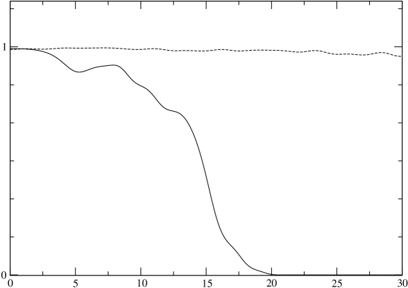
Figure 1: Squared modulus of the overlap between two neighbouring states $|\langle x_{1}(t),y_{1}(t)|x_{2}(t),y_{2}(t)\rangle|^{2}$ in the MFA for mean energy E=8.5, J=9/2 in a resonant ($\epsilon=1=\omega$) non integrable case with G=0.5, $G^{\prime}=0.2$ for conditions in the chaotic region (continuous lines) and regular region(dashed line). Chaotic initial conditions $(x_{1},y_{1})=(5.7263433,-0.24253563)$, $(x_{2},y_{2})=(5.7778567,-0.26845243)$. Regular initial conditions $(x_{1},y_{1})=(3.615516,0.53452248)$, $(x_{2},y_{2})=(3.68977334,0.50086791)$.

The authors are grateful to E.V. Passos and M.P. Pato for fruitful discussions. This work was partly funded by FAPESP, CNPq and PRONEX (Brazil), and Colciencias, DINAIN (Colombia). K.M.F.R. gratefully acknowledges the Instituto de F’ısica, Universidade de São Paulo, for their hospitality and PRONEX for partial support.

References

- [1] W.H. Zurek.Phys. Rev. D 24, 1516 (1981). For recent reviews J.M. Raimond et.al., Rev. Mod. Phys. 73, 565 (2001); A. Zeilinger, Rev. Mod. Phys. 71, S281 (1999) and references there in.
- [2] O. Bohigas et.al., Phys. Rev. Lett. 52, 1 (1984).
- [3] M.C. Gutzwiller. J. Math. Phys. 12, 343 (1971).
- [4] W.H. Zurek, and J.P. Paz, Physica (Amsterdam) 83D, 300 (1995)
- [5] K. Furuya et.al., Phys. Rev. Lett. 80, 5524 (1998).
- [6] P.A. Miller and S. Sarkar, Phys. Rev. E 60, 1542 (1999).