Quantum Characterization of a Werner-like Mixture

Abstract

We introduce a Werner-like mixture [R. F. Werner, Phys. Rev. A 40, 4277 (1989)] by considering two correlated but different degrees of freedom, one with discrete variables and the other with continuous variables. We evaluate the mixedness of this state, and its degree of entanglement establishing its usefulness for quantum information processing like quantum teleportation. Then, we provide its tomographic characterization. Finally, we show how such a mixture can be generated and measured in a trapped system like one electron in a Penning trap.

I Introduction

It is nowadays well known that the nonlocal properties of Quantum Mechanics [1, 2] enable striking processes in quantum information [3]. In these processes it is prominent the role of maximally entangled states [4, 5]. However, very often, the decoherence effects due to the environment transform the pure entangled state into a statistical mixture and degrade quantum entanglement in the real world [6]. Although purification schemes may be applied to noisy channels [7], there exist some mixture states which maintain interesting properties. An illuminating example is provided by the Werner mixture [8], which is not a mixture of product states, nonetheless not violating any Bell’s inequality [2], but still useful for quantum information processing [9, 10]. Such states belong to systems with two discrete degrees of freedom like two spin-$\frac{1}{2}$. However, information processing may sometimes involve hybrid systems where one degree of freedom has discrete variables and the other continuous variables. It may happen, for instance, in trapped ions [11, 12], or in trapped electrons [13] or in cavity quantum electrodynamics [14, 15]. Thus, it will be the aim of this paper to consider a mixture, which resembles the Werner one, but one of the two subsystems is described by continuous variables.

On the other hand, states and processes used in quantum information typically need of a well characterization [3]. This can be accomplished by using tomographic techniques [16]. Concerning the quantum state measurement, after the seminal work by Vogel and Risken [16], a lot of progress has been obtained and further techniques and algorithms were developed [17]. We would just mention the possibility of state reconstruction, for a composite system of discrete and continuous variables, by simply measuring the set of rotated spin projections and displaced number operators, [18, 19]. Then, we shall provide the tomographic characterization of a Werner-like mixture by generalizing that method.

The outline of the paper is the following: In Section II we discuss the Werner mixture and we extend the concept by considering one of the two subsystems with continuous variable. Then we characterize such a state in terms of mixedness and entanglement. Section III is devoted to the tomographic method employed for such a state reconstruction. In Section IV we present the results of numerical simulations. Finally, in Section V we discuss a possible implementation and Section VI is devoted to conclusions.

II Werner-like mixture

In his pioneering paper, Bell proved that a local realistic interpretation of Quantum Mechanics is impossible [2], and for the case of pure states it is known that, when measurements are performed on two quantum systems separated in space, their results are correlated in a manner which, in general, cannot be explained by a local hidden variables model [20]. Since the only pure states satisfying the Bell inequality are pure product states, one might naively think that the only mixed states that do not violate Bell’s inequality are mixtures of product states. However, Werner [8] showed that this conjecture is false for the so-called Werner states

$$\rho=\frac{1}{8}I_{1}\otimes I_{2}+\frac{1}{2}|\Psi^{-}\rangle\langle\Psi^{-}|\,,$$ (1)

where $I_{i}$ ($i=1,2$) stands for the identity operator of a single qubit ($|\downarrow\rangle_{i}{}_{i}\langle\downarrow|+|\uparrow\rangle_{i}{}_{i}\langle\uparrow|$) and $|\Psi^{-}\rangle=\frac{1}{\sqrt{2}}\left(|\downarrow\rangle_{1}|\uparrow\rangle_{2}-|\uparrow\rangle_{1}|\downarrow\rangle_{2}\right)$ is the spin singlet state.

A more general Werner mixture can be obtained by considering one of the two subsystems, say $2$, as described by continuous variables. A way to encode qubit in continuous variable systems could be the use of even and odd cat states which are orthogonal [21], thus resulting in the same situation of Eq.(1). Instead, the choice we are going to make is more general and gives the possibility to explore a variety of situations.

That is, we now replace the states $|\uparrow\rangle_{2}$, $|\downarrow\rangle_{2}$ of the second qubit with $|\alpha\rangle_{2}$ and $|-\alpha\rangle_{2}$, where the latter are coherent states of amplitude $\alpha$ and $-\alpha$ respectively (we shall consider $\alpha\in{\bf R}$ throughout the paper for the sake of simplicity). Therefore, a Werner-like mixture would be

$$\rho = \frac{1}{8}\left\{|\downarrow\rangle_{1}{}_{1}\langle\downarrow|\otimes|-\alpha\rangle_{2}{}_{2}\langle-\alpha|\right.$$ (6)

$$\left.+|\uparrow\rangle_{1}{}_{1}\langle\uparrow|\otimes|-\alpha\rangle_{2}{}_{2}\langle-\alpha|\right.$$

$$\left.+|\downarrow\rangle_{1}{}_{1}\langle\downarrow|\otimes|\alpha\rangle_{2}{}_{2}\langle\alpha|\right.$$

$$\left.+|\uparrow\rangle_{1}{}_{1}\langle\uparrow|\otimes|\alpha\rangle_{2}{}_{2}\langle\alpha|\right\}$$

$$+\frac{1}{4}\left[|\downarrow\rangle_{1}|\alpha\rangle_{2}-|\uparrow\rangle_{1}|-\alpha\rangle_{2}\right]\left[{}_{1}\langle\downarrow|{}_{2}\langle\alpha|-{}_{1}\langle\uparrow|{}_{2}\langle-\alpha|\right]\,.$$

Since $\langle\alpha|-\alpha\rangle=\exp(-2\alpha^{2})\neq 0$, the above state doesn’t describe a real two qubit system, but rather a two qubit system with nonorthogonal states [22]. Of course, for $\alpha\gg 1$ Eq.(6) behaves like the state (1), but we want to study its characteristics for a generic value of $\alpha$. To this end, we map the above state in the two spin-$\frac{1}{2}$ Hilbert spaces by introducing for the subsystem $2$ a vector $|\psi\rangle_{2}=\kappa|\downarrow\rangle_{2}$ $+\sqrt{1-\kappa^{2}}|\uparrow\rangle_{2}$ and considering the non orthogonal states $|\downarrow\rangle_{2}\,,|\psi\rangle_{2}$ instead of $|-\alpha\rangle_{2}\,,|\alpha\rangle_{2}$, with $\langle\psi|\downarrow\rangle=\kappa\equiv\exp(-2\alpha^{2})$. Then, Eq.(6) can be rewritten as

$$\rho = \frac{1}{8}\left\{|\downarrow\rangle_{1}{}_{1}\langle\downarrow|\otimes|\downarrow\rangle_{2}{}_{2}\langle\downarrow|\right.$$ (12)

$$\left.+|\uparrow\rangle_{1}{}_{1}\langle\uparrow|\otimes|\downarrow\rangle_{2}{}_{2}\langle\downarrow|\right.$$

$$\left.+|\downarrow\rangle_{1}{}_{1}\langle\downarrow|\otimes|\psi\rangle_{2}{}_{2}\langle\psi|\right.$$

$$\left.+|\uparrow\rangle_{1}{}_{1}\langle\uparrow|\otimes|\psi\rangle_{2}{}_{2}\langle\psi|\right\}$$

$$+\frac{1}{4}\left[|\downarrow\rangle_{1}|\psi\rangle_{2}-|\uparrow\rangle_{1}|\downarrow\rangle_{2}\right]\left[{}_{1}\langle\downarrow|{}_{2}\langle\psi|-{}_{1}\langle\uparrow|{}_{2}\langle\downarrow|\right]\,.$$

The degree of mixedness of the state (12) can be evaluated by using the Von Neumann entropy [23]

$$S(\rho)=-{\rm Tr}\left(\rho\log_{2}\rho\right)=-\sum_{i}\lambda_{i}\log_{2}\lambda_{i}\,,$$ (14)

where $\lambda_{i}$ are the eigenvalues of the matrix representation of $\rho$. We have calculated such eigenvalues in the basis ${\cal B}\equiv$ $\{|\downarrow\rangle_{1}|\downarrow\rangle_{2}$, $|\downarrow\rangle_{1}|\uparrow\rangle_{2}$, $|\uparrow\rangle_{1}|\downarrow\rangle_{2}$, $|\uparrow\rangle_{1}|\uparrow\rangle_{2}\}$ and we have plotted the entropy $S$ in Fig.1.

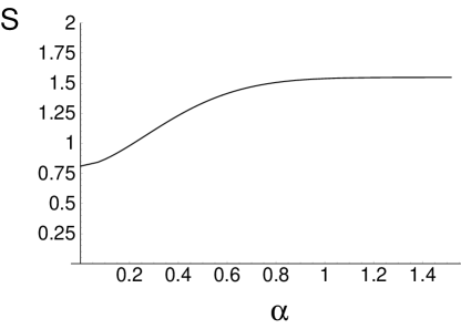
FIG. 1.: Entropy $S$ as function of $\alpha\equiv\sqrt{-(1/2)\ln\kappa}$.

We can see that also for $\alpha=0$ the state is a mixture, then, it becomes more and more mixed by increasing the value of $\alpha$, but never reaching the maximum (a completely mixed density operator in a $d$-dimensional space has entropy $\log_{2}d$). It is also worth noting that for $\alpha$ ($\kappa$) arbitrary, Eq.(12) is not a mixture of Bell’s states as it is for the Werner mixture (1), i.e., for $\alpha\gg 1$.

Let us now consider the measure of entanglement. For a two spin-$\frac{1}{2}$ system the state separability is related to the partial transposition operation [4, 24]. The matrix elements of partial transposition $\rho^{T_{2}}$ of a state $\rho$ are given by $\rho_{m\mu,\,n\nu}^{T_{2}}\equiv\rho_{m\nu,\,n\mu}$ where $\rho_{m\mu,\,n\nu}={}_{1}\langle m|{}_{2}\langle\mu|\rho|\nu\rangle_{2}|n\rangle_{1}$ with $m,n,\mu,\nu=\uparrow,\downarrow$. A density matrix $\rho$ for a two spin-$\frac{1}{2}$ system is inseparable if and only if its partial transpose, $\rho^{T_{2}}$, has any negative eigenvalue [4, 24]. Then, a suitable measure of entanglement can be defined as [25]

$$E(\rho)=-2\sum_{i}\lambda_{i}^{-}\,,$$ (15)

where $\lambda_{i}^{-}$ is a negative eigenvalue of $\rho^{T_{2}}$. It is worth noting that this measure satisfies the necessary conditions required for every measure of entanglement [5]. Then, we have plotted in Fig.2 the quantity $E$ calculated by exploiting again the matrix representation of Eq.(12) in the basis ${\cal B}$.

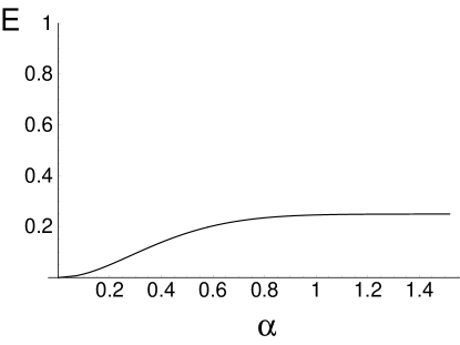
FIG. 2.: Degree of entanglement $E$ as function of $\alpha\equiv\sqrt{-(1/2)\ln\kappa}$.

We can see that the Werner-like mixture is factorisable for $\alpha=0$, then, by increasing $\alpha$, its degree of entanglement increases saturating at the value $1/4$ characteristic of the true Werner mixture (1). This latter value of entanglement is known to be sufficient to improve the teleportation performances over classical limit once the sender (Alice) and the receiver (Bob) initially share the state (1) [9]. Thus, it is straightforward to ask to what extent a Werner-like mixture can be used for the same goal. To establish a threshold value for $\alpha$ we are going to consider the teleportation fidelity. To this end, we first write the state $\rho$ through the Hilbert-Schmidt decomposition

$$\rho=\frac{1}{4} \left[I_{1}\otimes I_{2}+{\bf r}{\bf\cdot}\mbox{\boldmath$\sigma$}^{(1)}\otimes I_{2}+I_{1}\otimes{\bf s}{\bf\cdot}\mbox{\boldmath$\sigma$}^{(2)}\right.$$ (17)

$$\left.+\sum_{n,m=1}^{3}t_{n,m}\sigma_{n}^{(1)}\otimes\sigma_{m}^{(2)}\right]\,,$$

where $\{\sigma_{n}\}_{n=1,2,3}$ are the standard Pauli matrices, ${\bf r}$, ${\bf s}$ are vectors in ${\bf R}^{3}$ and ${\bf r}{\bf\cdot}\mbox{\boldmath$\sigma$}=\sum_{i=1}^{3}r_{i}\sigma_{i}$. Furthermore, the coefficients $t_{n,m}={\rm Tr}[\rho\,\sigma_{n}^{(1)}\otimes\sigma_{m}^{(2)}]$ form the real matrix $T$ describing the correlations between the two qubits. Thus, the teleportation capabilities will depend on the specific form of $T$. In particular it is shown in Ref.[26] that the teleportation fidelity amounts to

$$F=\frac{1}{2}\left[1+\frac{1}{3}{\rm Tr}\sqrt{T^{{\dagger}}T}\right]\,.$$ (18)

Then, in Fig.3 we have plotted the quantity $F$ versus $\alpha$ compared with the classical fidelity $2/3$.

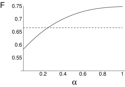
FIG. 3.: Teleportation fidelity as function of $\alpha\equiv\sqrt{-(1/2)\ln\kappa}$. The dashed line represents the classical bound of $2/3$.

We immediately recognize the presence of a threshold value ($\alpha=0.2476$) below which the Werner-like mixture becomes useless for quantum teleportation.

III State measurement

We now discuss the possibility of a complete characterization of the Werner-like mixture through tomographic techniques. In particular, we generalize the method presented in Refs.[18, 19] to non pure states.

Accordingly to the state reconstruction principle developed in Ref.[27] we choose an observable, here $\sigma_{3}\otimes a^{{\dagger}}a$, then we apply suitable unitary transformations to get a set of observables giving the whole state information upon measurements. In our case the transformations would be

$$U(\theta,\varphi) = \exp\left[-i\theta\left(\sigma_{1}\cos\varphi+\sigma_{2}\sin\varphi\right)\right]\,,$$ (19)

$$D(\beta) = \exp\left[\beta a^{{\dagger}}-\beta^{*}a\right]\,,$$ (20)

which lead to rotated (by angles $\theta$ and $\varphi$) spin projection in the subsystem $1$ [28], and to displaced number state (by a complex amount $\beta$) in the subsystem $2$ [29]. Then, it is possible to consider the following measurable marginal distributions

$$w(s,n;\theta,\varphi,\beta) = {\rm Tr}\left\{\rho\,D(\beta)U(\theta,\varphi)\right.$$ (22)

$$\left.|s\rangle_{1}{}_{1}\langle s|\otimes|n\rangle_{2}{}_{2}\langle n|U^{{\dagger}}(\theta,\varphi)D^{{\dagger}}(\beta)\right\}\,,$$

having as variables the eigenvalues $s$, $n$ of $\sigma_{3}$ and $a^{{\dagger}}a$ as variables and parametrically depending on $\theta$, $\varphi$ and $\beta$. Thus, measuring the state $\rho$ would mean the possibility to express $\rho$ as a functional operator of $w$, i.e. to invert expression (22). This also means the possibility to sample the density matrix elements (in some basis) from the quantity measured by spanning the whole space of parameters.

In reality, we shall see that it is not necessary to consider all possible values of parameters. As matter of fact, we write the density operator (6) as

$$\rho=\left[\begin{array}[]{cc}\rho^{\uparrow\uparrow}&\rho^{\uparrow\downarrow}\\ \rho^{\downarrow\uparrow}&\rho^{\downarrow\downarrow}\end{array}\right]\,,\quad\rho^{\downarrow\uparrow}=[\rho^{\uparrow\downarrow}]^{{\dagger}}\,,$$ (24)

where each operator $\rho^{\uparrow\uparrow}$, $\rho^{\uparrow\downarrow}$, $\rho^{\downarrow\uparrow}$, $\rho^{\downarrow\downarrow}$, can in turn be represented in the Fock basis of the subsystem $2$.

Now, we set $\theta=\varphi=0$ and we suppose to retain only the measurement results $s=\uparrow$; then, expanding the density operator $\rho^{\uparrow\uparrow}$ in the Fock basis, and defining $N_{c}$ as an appropriate estimate of the maximum number of excitations (cut-off), we have

$$w(\uparrow,n;0,0,\beta)=\sum_{k,m=0}^{N_{c}}\langle n,\beta|k\rangle\langle k|\rho^{\uparrow\uparrow}|m\rangle\langle m|n,\beta\rangle\,.$$ (25)

The projection of the displaced number state $|n,\beta\rangle$ onto the Fock state $|m\rangle$ can be obtained generalizing the result derived in Ref. [30].

Let us now consider, for a given value of $|\beta|$, $w$ as a function of $\phi=\arg[\beta]$ [31] and calculate the coefficients of the Fourier expansion

$$w(\uparrow,n;0,0,r)=\frac{1}{2\pi}\int_{0}^{2\pi}d\phi\;w(\uparrow,n;0,0,\phi)e^{ir\phi}\;,$$ (26)

for $r=0,1,2,\ldots$. Combining Eqs. (25) and (26), we get

$$w(\uparrow,n;0,0,r)=\sum_{m=0}^{N_{c}-r}{G}^{(r)}_{n,m}(|\beta|)\langle m+r|\rho^{\uparrow\uparrow}|m\rangle\,,$$ (27)

where the explicit expression of the matrices $G$ is given in Ref. [18].

We may now notice that if the distribution $w(\uparrow,n;0,0,\beta)$ is measured for $n\in[0,N]$ with $N\geq N_{c}$, then Eq. (27) represents, for each value of $r$, a system of $N+1$ linear equations between the $N+1$ measured quantities and the $N_{c}+1-r$ unknown density matrix elements. Therefore, in order to obtain the latter, we only need to invert the system

$$\langle m+r|\rho^{\uparrow\uparrow}|m\rangle=\sum_{n=0}^{N}M^{(r)}_{m,n}(|\beta|)w(\uparrow,n;0,0,r)\,,$$ (28)

where the matrices $M$ are given by $M=(G^{T}G)^{-1}G^{T}$.

The procedure can be repeated with $w(\downarrow,n;0,0,\beta)$ in order to get the matrix elements of $\rho^{\downarrow\downarrow}$. Then, changing the parameters so that $\theta=\pi/4$ and $\varphi=-\pi/2$ we can get the real part of the matrix elements of $\rho^{\uparrow\downarrow}$. Instead, with $\theta=\pi/4$ and $\varphi=0$ we can get the imaginary part of the matrix elements of $\rho^{\uparrow\downarrow}$, thus concluding the reconstruction procedure of the state (24).

IV Numerical results

As an example of the proposed method, we show in Figs. 4, 5, 6 the results of numerical Monte-Carlo simulations of the reconstruction of the state (6) once written in the form (24). In this simulation we have used the value $\alpha=0.7$ which make the state different from a true Werner mixture, but still having nonclassical features as discussed in Section II.

In order to account for experimental conditions, we have also considered the effects of a non-unit quantum efficiency $\eta$ in the counting of the number of excitations. When $\eta<1$, the actually measured distribution is related to the ideal distribution by a binomial convolution [32].

Statistical errors are accounted for as well by considering an estimation of the marginal distributions given by $w^{\rm est}(n;\phi)={\cal N}_{\phi}(n)/{\cal N}_{\phi}$, where ${\cal N}_{\phi}(n)$ is the number of events with $n$ counts at phase $\phi$, while ${\cal N}_{\phi}$ is the total number of events at the same phase. Then, following the arguments given in Refs.[31, 33], the quantities ${\cal N}_{\phi}(n)$ can approximately be regarded as independent Poissonian random variables, whose means and variances are given by $w(n;\phi){\cal N}_{\phi}\approx w^{\rm est}(n;\phi){\cal N}_{\phi}$. The variance of $w^{\rm est}(n;\phi)$ may then be approximated by $w^{\rm est}(n;\phi)/{\cal N}_{\phi}$, so that the variances of the real and imaginary parts of the density matrix can be easily estimated using Eq.(28) (and similarly for the other density operators). This means that the errors can be estimated in real time as the experiment runs, simultaneously with the reconstruction of the density matrix elements.

Other error sources leading to discrepancies between true and reconstructed density matrices can be identified in the choice of $|\beta|$, $N_{c}$ and $N_{\phi}$ (number of phases). However, as it can be seen from Figs. 4, 5, 6 the reconstructed density matrices turn out to be quite faithful.

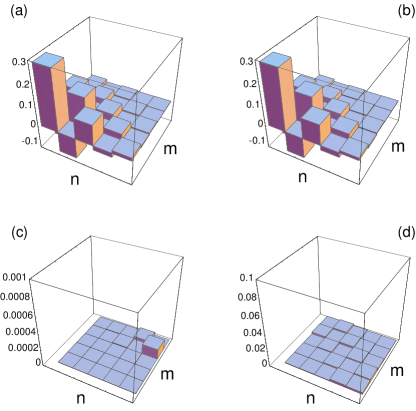
FIG. 4.: Density matrix elements of $\rho^{\uparrow\uparrow}$ for the state (6) with $\alpha=0.7$. In the computer simulation $N_{\phi}=96$ phases are considered and ${\cal N}_{\phi}=10^{4}$ measurement events at each phase are assumed to be recorded using $N_{c}=31$. The other parameters are $|\beta|=0.6$ and $\eta=0.9$. (a) Exact density matrix; (b) reconstructed density matrix; (c) statistical errors; (d) absolute difference between reconstructed and exact density matrix elements.

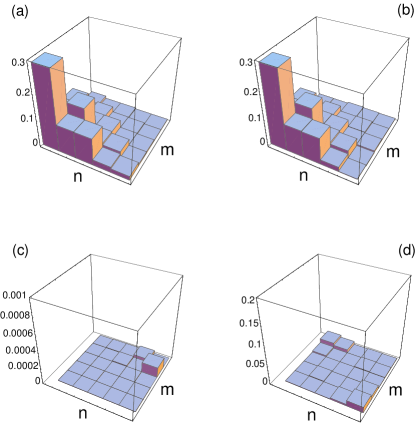
FIG. 5.: Density matrix elements of $\rho^{\downarrow\downarrow}$ for the state (6) with $\alpha=0.7$. In the computer simulation $N_{\phi}=96$ phases are considered and ${\cal N}_{ev}=10^{4}$ measurement events at each phase are assumed to be recorded using $N_{c}=31$. The other parameters are $|\beta|=0.6$ and $\eta=0.9$. (a) Exact density matrix; (b) reconstructed density matrix; (c) statistical errors; (d) absolute difference between reconstructed and exact density matrix elements.

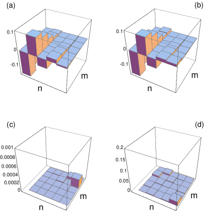
FIG. 6.: Density matrix elements of $\rho^{\uparrow\downarrow}$ for the state (6) with $\alpha=0.7$. In the computer simulation $N_{\phi}=96$ phases are considered and ${\cal N}_{ev}=10^{4}$ measurement events at each phase are assumed to be recorded using $N_{c}=31$. The other parameters are $|\beta|=0.6$ and $\eta=0.9$. (a) Exact density matrix; (b) reconstructed density matrix; (c) statistical errors; (d) absolute difference between reconstructed and exact density matrix elements.

In addition to the present case we have performed other simulations with different values of $\alpha$ and several values of the parameters, which confirm that the present method is quite stable and accurate.

The phase-space description corresponding to (24) is given by the Wigner-function matrix [34]

$$W = \left[\begin{array}[]{cc}W^{\uparrow\uparrow}(\gamma)&W^{\uparrow\downarrow}(\gamma)\\ W^{\downarrow\uparrow}(\gamma)&W^{\downarrow\downarrow}(\gamma)\end{array}\right]$$ (31)

$$= \left[\begin{array}[]{cc}{\rm Tr}_{2}[\rho^{\uparrow\uparrow}\,\delta(\gamma-\hat{a})]&{\rm Tr}_{2}[\rho^{\uparrow\downarrow}\,\delta(\gamma-\hat{a})]\\ {\rm Tr}_{2}[\rho^{\downarrow\uparrow}\,\delta(\gamma-\hat{a})]&{\rm Tr}_{2}[\rho^{\downarrow\downarrow}\,\delta(\gamma-\hat{a})]\end{array}\right]\,,$$ (34)

where $\delta(\gamma-\hat{a})$ is the Fourier transform of the displacement operator [30].

Then, the Wigner functions corresponding to the density matrices of Figs.4, 5 and 6, are shown in Figs.7 and 8.

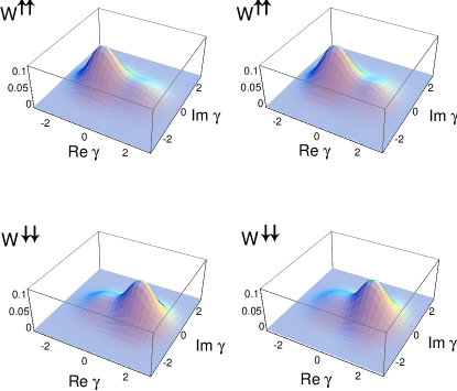
FIG. 7.: Top: Wigner function corresponding to the density matrix of Fig.4 (true on the left and reconstructed on the right). Bottom: Wigner function corresponding to the density matrix of Fig.5 (true on the left and reconstructed on the right).

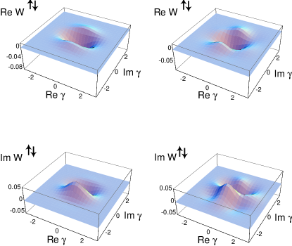
FIG. 8.: Wigner function corresponding to the density matrix of Fig.6 (true on the left and reconstructed on the right).

The reconstructed Wigner functions as well turn out to be quite faithful. We would like to emphasize their particular shape. In $W^{\uparrow\uparrow}$ there are two hills, one centered in ${\rm Re}\,\gamma=-\alpha$ and the other in ${\rm Re}\,\gamma=\alpha$ coming from the random part of the state (6), instead, the pseudo singlet part of the state contributes only to the bump in $-\alpha$, thus producing the asymmetric effect. The opposite happens for $W^{\downarrow\downarrow}$. The shape of $W_{\uparrow\downarrow}$ is due to the quantum interference given by the entanglement between the two degrees of freedom: in fact, in absence of entanglement $\rho^{\uparrow\downarrow}$ would just be a replica of the diagonal parts $\rho^{\uparrow\uparrow}$ and $\rho^{\downarrow\downarrow}$.

V Physical Realization

We now briefly discuss a system where the Werner-like mixture could be synthesized and even measured. It is a single electron trapped in a Penning trap [35], where two different degrees of freedom of the same particle can be entangled and also measured.

An electron in a Penning trap is confined by the combination of a homogeneous magnetic field along the positive $z$ axis and an electrostatic quadrupole potential in the $xy$ plane [35]. The spatial part of the electronic wave function consists of three degrees of freedom, neglecting the slow magnetron motion (whose characteristic frequency lies in the kHz region), here we only consider the axial and cyclotron motions, which are two harmonic oscillators radiating in the MHz and GHz regions, respectively. On the other hand, the spin dynamics results from the interaction between the magnetic moment of the electron and the static magnetic field, so that the free Hamiltonian reads as [35]

$$H_{\rm free}=\hbar\omega_{z}a_{z}^{{\dagger}}a_{z}+\hbar\omega_{c}a_{c}^{{\dagger}}a_{c}+\hbar\omega_{s}\sigma_{3}/2\,,$$ (35)

where the indices $z$, $c$, and $s$ refer to the axial, cyclotron and spin motions, respectively.

Here, in addition to the usual trapping fields, we consider an external radiation field as a standing wave along the $z$ direction and rotating, i.e. circularly polarized, in the $xy$ plane with frequency $\Omega$ [36]. To be more specific, we consider a standing wave within the cylindrical cavity configuration [37] with the (dimensionless) wave vector $k$. Then, the interaction Hamiltonian reads [36]

$$H_{\rm int} = \hbar\epsilon\left[a_{c}e^{i(\Omega t+\varphi)}+a_{c}^{{\dagger}}e^{-i(\Omega t+\varphi)}\right]\cos(kz+\chi)$$ (36)

$$+ \hbar\zeta\left[\sigma_{-}e^{i(\Omega t+\varphi)}+\sigma_{+}e^{-i(\Omega t+\varphi)}\right]\sin(kz+\chi)\;,$$ (37)

where $\sigma_{\pm}=(\sigma_{1}\pm i\sigma_{2})/2$, and $z=a_{z}+a_{z}^{\dagger}$. The phase $\chi$ defines the position of the center of the axial motion with respect to the wave. Depending on its value the electron can be positioned in any place between a node ($\chi=0$) and an antinode ($\chi=\pm\pi/2)$. Instead, the phase $\varphi$ is related to the initial direction of the electric (magnetic) field in the $xy$ plane, or to the phase of any reference field. The two coupling constants $\epsilon$ and $\zeta$ are proportional to the amplitude of the applied radiation field. Depending on $\Omega$ and $\chi$, the interaction Hamiltonian (36) gives rise to different contributions at leading order in the Taylor expansion of $\sin(kz+\chi)$ and $\cos(kz+\chi)$.

We immediately recognize the possibility of implementing the transformations (19), (20) on the spin and cyclotron degrees of freedom by appropriately exploiting the Hamiltonian (36). For instance, $U$ can be realized by setting $\Omega=\omega_{s}$, $\chi=0$, and then adjusting $\varphi$ and $\theta=\zeta t$. Differently, $D$ can be realized by setting $\Omega=\omega_{c}$, $\chi=-\pi/2$, and then adjusting $\beta=\epsilon te^{-i\varphi}$.

These transformations easily allow to generate the disentangled components of the mixture (6), i.e., $|\uparrow\rangle_{1}|\pm\alpha\rangle_{2}$ and $|\downarrow\rangle_{1}|\pm\alpha\rangle_{2}$, starting from the typical initial state $|\uparrow\rangle_{1}|0\rangle_{2}$.

Instead, for what concerns the generation of the entangled fraction of the mixture (6), we recall the procedure developed in Ref.[18]. That is, we consider the possibility of introducing pulsed standing waves through the microwave inlet [35] so that $\epsilon$, $\zeta$ become time dependent and $\tilde{\epsilon}$, $\tilde{\zeta}$ indicate the pulse area (the duration of the pulse is assumed to be much shorter than the characteristic axial period, which is of the order of microseconds). Then, nonclassical cyclotron states can be entangled with the spin states through the following steps [18].

• First, we consider $\chi=0$, $\Omega=\omega_{s}$, and a pulsed standing wave lasting $\Delta t_{1}=t_{1}-t_{0}=t_{1}$;

• Second, we allow a free evolution for a time $\Delta t_{2}=t_{2}-t_{1}=\pi/(2\omega_{z})$;

• Third, we consider the action of another pulsed standing wave with $\chi=-\pi/2$, $\Omega=\omega_{c}$, for a time $\Delta t_{3}=t_{3}-t_{2}$.

Finally, if we consider the initial axial state as a Gaussian state with momentum width much smaller than ${\tilde{\zeta}}$ (which is easily obtained in the case of the ground state of the axial oscillator), we end up with an evolution operator of the form $D(\alpha\sigma_{1})$, where $\alpha$ is related to ${\tilde{\epsilon}}$, ${\tilde{\zeta}}$ and $\varphi$. It is then immediate to see that the initial state $|\uparrow\rangle_{1}|0\rangle_{2}$ may evolve with the aid of $D(\alpha\sigma_{1})$ and a spin rotation into

$$\frac{1}{\sqrt{2}}\left(|\downarrow\rangle_{1}|\alpha\rangle_{2}-|\uparrow\rangle_{1}|-\alpha\rangle_{2}\right)\,.$$ (38)

This state has been already discussed in Refs. [12, 15] and constitutes the pseudo singlet component of the mixture (6).

Thus, at each run of the experiment the desired component of the Werner-like mixture can be synthesized, thus allowing the generation of the state (6) on average ensemble.

For what concerns the measurement, the addition of a particular inhomogeneous magnetic field (known as the magnetic bottle field [35]) to that already present in the trap, allows to perform a simultaneous measurement of both the spin and the cyclotron excitations number. The useful interaction Hamiltonian for the measurement process is

$$H_{\rm bottle}=\hbar\omega_{b}\left[a^{{\dagger}}_{c}a_{c}+\frac{g}{2}\sigma_{3}\right]z^{2}\,,$$ (39)

where the angular frequency $\omega_{b}$ is directly related to the strength of the magnetic bottle field.

Equation (39) describes the fact that the axial angular frequency is affected both by the number of cyclotron excitations $a_{c}^{{\dagger}}a_{c}$ and by the eigenvalue of $\sigma_{3}$. The modified (shifted) axial frequency can be experimentally measured [35] after the application of the inhomogeneous magnetic bottle field. One immediately sees that it assumes different values for every pair of eigenvalues of $a_{c}^{{\dagger}}a_{c}$ and $\sigma_{3}$ due to the fact that the electron $g$ factor is slightly (but measurably [35]) different from $2$.

However, prior such kind of measurement, one has to deal with the transformations (19), (20) which can be realized through the Hamiltonian (36) as discussed above.

Repeating this procedure many times allows us to recover the desired marginal distributions, hence to sample the density matrix elements.

VI Conclusions

In conclusions, we have studied the properties of a Werner-like mixture and a reliable method to achieve its tomographic characterization. A useful system to investigate such states has been individuated in the trapped electron. There are other candidate systems that offer the possibility to generate and manipulate the studied state. We mention for example trapped ions [11], or atoms in cavity quantum electrodynamics [14]. Moreover, in such systems the studied state might involve two particles, or quite generally the two subsystems could be spatially separated.

The experimental studies on this state might yield new insight in the foundations of quantum mechanics and allow further progress in the field of quantum information.

REFERENCES

- [1] A. Einstein, B. Podolsky and N. Rosen, Phys. Rev. 47, 777 (1935).
- [2] J. S. Bell, Physics 1, 195 (1965).
- [3] M. A. Nielsen and I. L. Chuang, Quantum Computation and Quantum Information, (Cambridge University Press, Cambridge, 2000).
- [4] A. Peres, Phys. Rev. Lett; 77, 1413 (1996).
- [5] V. Vedral, M. B. Plenio, M. A. Rippin and P. L. Knight, Phys. Rev. Lett. 78, 2275 (1998); V. Vedral and M. B. Plenio, Phys. Rev. A 57, 1619 (1998).
- [6] W. H. Zurek, Phys. Today 44(10) (1991); A. Royer, Phys. Rev. Lett. 77, 3272 (1996).
- [7] C. H. Bennet, G. Brassard, S. Popescu, B. Schumacher, J. A. Smolin and W. K. Wootters, Phys. Rev. Lett. 76, 722 (1996).
- [8] R. F. Werner, Phys. Rev. A 40, 4277 (1989).
- [9] S. Popescu, Phys. Rev. Lett. 72, 797 (1994).
- [10] C. Bennett, H. J. Bernstein, S. Popescu and B. Schumacher, Phys. Rev. A 53, 2046 (1996); C. H. Bennett, D. P. DiVincenzo, J. A. Smolin and W. K. Wooters, Phys. Rev. A 54, 3824 (1996).
- [11] C. Monroe, D. M. Meekhof, B. E. King, W. M. Itano and D. J. Wineland, Phys. Rev. Lett. 75, 4714 (1995).
- [12] C. Monroe, D. M. Meekhof, B. E. King and D. J. Wineland, Science 272, 1131 (1996).
- [13] S. Mancini, A. M. Martins and P. Tombesi, Phys. Rev. A 61, 012303 (2000).
- [14] P. Domokos, J. M. Raimond, M. Brune and S. Haroche, Phys. Rev. Lett. 52, 3554 (1995).
- [15] M. Brune, E. Hagley, J. Dreyer, X. Maitre, A. Maali, C. Wunderlich, J. M. Raimond and S. Haroche, Phys. Rev. Lett. 77, 4887 (1996); J. M. Raimond, M. Brune and S. Haroche, Phys. Rev. Lett. 79, 1964 (1997).
- [16] K. Vogel and H. Risken, Phys. Rev. A 40, 7113 (1989).
- [17] Special issue of J. Mod. Opt. 44, (1997); D. G. Welsch, W. Vogel and T. Opatrny, Progress in Optics 39, 65 (1999).
- [18] M. Massini, M. Fortunato, S. Mancini and P. Tombesi, Phys. Rev. A 62, 041401(R) (2000).
- [19] M. Massini, M. Fortunato, S. Mancini, P. Tombesi and D. Vitali, New Journal of Physics 2, 20.1 (2000).
- [20] N. Gisin and A. Peres, Phys. Lett. A 162, 15 (1992); S. Popescu and D. Rohrlich, Phys. Lett. A 166, 293 (1989).
- [21] P. T. Cochrane, G. J. Milburn and W. J. Munro, Phys. Rev. A 59, 2631 (1999); S. Mancini and V. I. Man’ko, arXiv:quant-ph/0111128 (to appear in J. Opt. B).
- [22] O. Hirota and M. Sasaki, Quantum Communication, Computing and Measurement 3, Ed. by P. Tombesi and O. Hirota (Kluwer/Plenum, New York, 2000), p.359; O. Hirota, S. J. van Enk, K. Nakamura, M. Sohma and K. Kato, arXiv:quant-ph/0101096.
- [23] J. von Neumann, Mathematical Foundations of Quantum Mechanics, (Princeton University Press, Princeton, 1955).
- [24] M. Horodecki, P. Horodecki and R. Horodecki, Phys. Lett. A 223, 1 (1996).
- [25] J. Lee and M. S. Kim, Phys. Rev. Lett. 84, 4236 (2000).
- [26] R. Horodecki, M. Horodecki and P. Horodecki, arXiv:quant-ph/9606027.
- [27] S. Mancini, V. I. Man’ko and P. Tombesi, J. Mod. Opt. 44, 2281 (1997).
- [28] S. Weigert, Phys. Phys. Rev. Lett. 84, 802 (2000); S. Weigert, Acta Phys. Slov. 49, 613 (1999); S. Mancini, M. Fortunato, P. Tombesi and G. M. D’Ariano, J. Opt. Soc. Am. A 17, 2529 (2000); V. I. Man’ko and O. V. Man’ko, Zh. Eksp. Teor. Fiz. 112, 796 (1997) [JETP 85, 430 (1997)].
- [29] K. Banaszek and K. Wodkiewicz, Phys. Rev. Lett; 76, 4344 (1996); S. Mancini, V. I. Man’ko and P. Tombesi, Europhys. Lett. 37, 79 (1997); S. Wallentowitz, R. L. de Matos Filho and W. Vogel, Phys. Rev. A 56, 1205 (1997).
- [30] K. E. Cahill and R. J. Glauber, Phys. Rev. 177, 1857 (1969); ibid. 1882 (1969).
- [31] T. Opatrný and D. G. Welsh, Phys. Rev. A 55, 1462 (1997).
- [32] M. O. Scully and W. E. Lamb, Phys. Rev. 179, 368 (1969).
- [33] U. Leonhardt, M. Munroe, T. Kiss, Th. Richter and M. G. Raymer, Opt. Comm. 127, 144 (1996).
- [34] M. Hillery et al Phys. Rep. 106, 121 (1986); S. Walletowitz et al. Phys. Rev. A 56, 1205 (1997).
- [35] L. S. Brown and G. Gabrielse, Rev. Mod. Phys. 58, 233 (1986).
- [36] A. M. Martins, S. Mancini and P. Tombesi, Phys. Rev. A 58, 3813 (1998).
- [37] G. Gabrielse and J. Tan, in Cavity Quantum Electrodynamics, edited by P. R. Berman, (Academic Press, San Diego, CA, 1994), p. 267.