Experimental realization of the Brüschweiler’s algorithm in a homo-nuclear system

Abstract

Compared with classical search algorithms, $Grover$ quantum algorithm [$Phys.$ $Rev.$ $Lett.$, 79, 325(1997)] achieves quadratic speedup and $Br\ddot{u}schweiler$ hybrid quantum algorithm [$Phys.$ $Rev.$ $Lett.$, 85, 4815(2000)] achieves an exponential speedup. In this paper, we report the experimental realization of the $Br\ddot{u}schweiler$ algorithm in a $3$-qubit NMR ensemble system. The pulse sequences are used for the algorithms and the measurement method used here is improved on that used by Brüschweiler, namely, instead of quantitatively measuring the spin projection of the ancilla bit, we utilize the shape of the ancilla bit spectrum. By simply judging the downwardness or upwardness of the corresponding peaks in an ancilla bit spectrum, the bit value of the marked state can be read out, especially, the geometric nature of this read-out can make the results more robust against errors.

PACS numbers: 03.67.Lx, 82.56.Jn, 76.60.-k.

I Introduction

Quantum algorithms are very important in quantum computing. One can find this point in Deutsch and Josza’s quantum algorithm which demonstrates the incomparable advantage of quantum computing [1]. Two more famous quantum algorithms which are closely related to practical applications of quantum computation are: Shor’s factoring algorithm [2] and Grover’s quantum search algorithm[3]. The factorization of a large number into prime factors is a difficult mathematical problem because existing classical algorithms require exponential times to complete the factorization in terms of the input. However, Shor’s quantum algorithm drastically decreases this to polynomial times. Another similar example is searching marked items from an unsorted database. Actually, many scientific and practical problems can be abstracted to such search problem. Hence it is a very important subject. Classically, it can only be done by exhaustive searching. Unlike Shor’s algorithm, Grover’s quantum algorithm achieves only quadratic speedup over classical algorithms, namely the number of searching is reduced from $O(N)$ to $O(\sqrt{N})$. However, it has been proven that Grover’s algorithm is optimal for quantum computing[4]. The strong restriction of the optimality theorem can be broken off if we go out of quantum computation and then exponential speedup may be achieved. Using nonlinear quantum mechanics, Abram and Lloyd[5] have constructed a quantum algorithm that achieves exponential speedup. However the applicability of nonlinear quantum mechanics is still under investigation, let alone the realization of their algorithm at present.

Recently, by using multiple-quantum operator algebra, Brüschweiler put forward a hybrid quantum search algorithm that combines DNA computing idea with the quantum computing idea [6]. The new algorithm achieves an exponential speedup in searching an item from an unsorted database. It requires the same amount of resources as effective pure state quantum computing. There are several known schemes for quantum computers, such as cooled ions[7], cavity QED[8], nuclear magnetic resonance[9] and so on. NMR technique is sophisticated and many quantum algorithms have been realized by using NMR system[10, 11, 12, 13, 14, 15, 16]. Many studies show that the NMR system is particularly suitable for the realization of such algorithms, in which ensembles of quantum nuclear spin system are involved. Strictly speaking, Brüschweiler algorithm is not a pure quantum algorithm, and thus the realization of Brüschweiler algorithm in NMR enjoys the freedom from the debate[17, 18] about the quantum nature of the NMR computation using effective pure state. Because this algorithm is exponentially fast, it tales much shorter time to finish a search problem and this also makes the algorithm more robust again decoherence.

In this paper, we report the experimental realization of $Br\ddot{u}schweiler$ algorithm in a 3-qubit homo-nuclear system. In the procedure, we have improved the measurement method used by Brüschweiler in his paper[6]. Instead of measuring the ancilla bit’s spin polarization, we utilize the shapes of ancilla bit’s spectra, $i.e.$ by judging the downwardness or upwardness of the corresponding peaks in the spectrum, the bit value of the marked state can be read out. Since the geometric property of the spectrum is easy to be recognized, this makes the algorithm more tolerant to errors. Our paper is organized as follows. After this introduction, we briefly describe Brüschweiler’s original algorithm in section II, and then we introduce our modification part based on $Br\ddot{u}schweiler$ algorithm in section III. In section IV, we present the details of the pulse sequences of the algorithm and the results of our experiment. Finally, a summary is given.

II Brüschweiler’s algorithm

NMR techniques lie far ahead of other suggested quantum computing technologies. However, during recent years, the rapid developing tendency becomes slow and slow. People have taken more effort in preparing an effective pure state, but compared with a pure state quantum computer, there is no essential speedup. Brüschweiler’s wonderful idea may shed a light on this area, he takes advantage of the mixed state nature in the NMR system and achieves an exponential speedup in searching an unsorted database. For convenience in following discussion, here we repeat the main idea of the Brüschweiler’s algorithm in brief (in detail, see Refs. [6, 21]).

As is well-known, the preparation of the effective pure state is one of the most troublesome part in a NMR quantum computing experiment. On the other hand, the effective pure state also sets a restriction on the number of qubits[19, 20]. The effective pure state is represented by the density operator

$$\rho=(1-\varepsilon)2^{-n}{\bf\hat{1}}+\varepsilon\left|00...0\right\rangle\left\langle 00...0\right|.$$ (1)

At room temperature, under the high temperature approximation we have

$$\varepsilon=\frac{nhv}{2^{n}kT}.$$ (2)

In Eq. (1), the second term’s contribution to the outcome is scaled by the factor $\varepsilon$, which decreases exponentially with $n$, namely, the number of qubit, but the first term has no contribution at all[22].

In NMR ensemble system, the state can be represented by density operators which are linear combinations of direct products of spin polarization operators [9, 21]. In a strong external magnetic field, the eigenstates of the Zeeman Hamiltonian

$$|\phi_{in}\rangle=\left|001...01\right\rangle\>=\left|\alpha\alpha\beta...\alpha\beta\right\rangle,$$ (3)

are mapped on states in the spin Liouville space

$$\sigma_{in}=\left|\phi\right\rangle\left\langle\phi\right|={I}_{1}^{\alpha}{I}_{2}^{\alpha}{I}_{3}^{\beta}...{I}_{n-1}^{\alpha}{I}_{n}^{\beta},$$ (4)

where

$${I}_{k}^{\alpha}=\left|\alpha^{k}\right\rangle\left\langle\alpha^{k}\right|={\frac{1}{2}}({\bf 1}_{k}+2{I}_{kz})=\left[\begin{array}[]{cc}1&0\\ 0&0\end{array}\right],$$ (5)

$${I}_{k}^{\beta}=\left|\beta^{k}\right\rangle\left\langle\beta^{k}\right|={\frac{1}{2}}({\bf 1}_{k}-2{I}_{kz})=\left[\begin{array}[]{cc}0&0\\ 0&1\end{array}\right],$$ (6)

represent respectively spin up and spin down state of the spin. Usually, the oracle or query is a computable function $f$: $f(x)=0$ for all $x$ except for $x=z$ which is the item that we want to find out for which $f(z)=1$. Usually, the oracle can be expressed as a permutation operation which is a unitary operation $U_{f}$, implemented using logic gates [6]. In Brüschweiler algorithm, an extra bit(also called the ancilla bit) is used and its state is represented by ${I}_{0}$. The output of the oracle is stored on the ancilla bit ${I}_{0}$ whose state is prepared in the $\alpha$ state at the beginning. The output of $f$ can be represented by an expectation value of ${I}_{0z}$ for a pure state

$$f=F({I}_{0}^{\alpha}\sigma_{in})={\frac{1}{2}}-Tr(U_{f}{I}_{0}^{\alpha}\sigma_{in}U_{f}^{+}{I}_{0z}).$$ (7)

If $\sigma_{in}$ happens to satisfy the oracle, then $I_{0}^{\alpha}$ is changed to $I_{0}^{\beta}$. This gives the value of the trace equal to $-1/2$, and hence $f$ equals to 1. The input of $f$ can be an mixed state of the form $\rho=\sum_{j=1}^{N}\;{I}_{0}^{\alpha}\;\sigma_{j}$ where $\sigma_{j}$ is one of the form in Eq. (4):

$$f=\sum\limits_{j=1}^{N}F({I}_{0}^{\alpha}\;\sigma_{j})=F(\sum\limits_{j=1}^{N}{I}_{0}^{\alpha}\;\sigma_{j})+{\frac{{N-1}}{2}}.$$ (8)

The oracle is applied simultaneously to all the components in the NMR ensemble. The oracle operation is quantum mechanical. Brüschweiler put forward two versions of search algorithm. We adopt his second version. The essential of the Brüschweiler algorithm is as follow: suppose that the unsorted database has $N=2^{n}$ number of items. We need $n$ qubit system to represents these $2^{n}$ items. The algorithm contains $n$ oracle queries each followed by an measurement:
(1) Each time, ${I}_{0}^{\alpha}{I}_{k}^{\alpha}$ ($k=1,2,...,n$) is prepared. In fact, the input state ${I}_{0}^{\alpha}...{\bf 1}...I_{k}^{\alpha}...{\bf 1}...$ is a highly mixed state[21]. In the following text, the identity operator will be omitted. This Liouville operator actually represents the $2^{n-1}$ number of items encoded in mixed state:

$${I}_{0}^{\alpha}{I}_{k}^{\alpha} = {I}_{0}^{\alpha}({I}_{1}^{\alpha}+{I}_{1}^{\beta})({I}_{2}^{\alpha}+{I}_{2}^{\beta})...({I}_{n}^{\alpha}+{I}_{n}^{\beta})$$ (9)

$$= \sum_{\gamma_{1},\gamma_{2},...,\gamma_{k-1},\gamma_{k},\gamma_{k+1},...,\gamma_{n}=\alpha,\beta}{I}_{0}^{\alpha}{I}_{1}^{\gamma_{1}}{I}_{2}^{\gamma_{2}}...{I}_{k-1}^{\gamma_{k-1}}{I}_{k}^{\alpha}{I}_{k+1}^{\gamma_{k+1}}...{I}_{n}^{\gamma_{n}}$$ (10)

$$= \sum_{i_{1},i_{2},...,i_{k-1},i_{k+1},...,i_{n}=0,1}\left|i_{1}i_{2}...i_{k-1}0i_{k+1}...i_{n}\right\rangle\>\left\langle i_{1}i_{2}...i_{k-1}0i_{k+1}...i_{n}\right|.$$ (11)

This mixed state contains half of the whole items in the database. The $k$-th bit is set to $\alpha$. The other half of the database with $k$-th bit equals to $\beta$(or 1) is not included. (2) Applying the oracle function to the system. As seen in eq. (8), the operation is done simultaneously to all the basis states. If $k$-th bit of the marked state is $0$, then the marked state is contained in eq. (11). One of the $2^{n}$ terms in equation (11) satisfies the oracle and the oracle changes the sign of the ancilla bit from $\alpha$ to $\beta$. If one measures the spin of ancilla spin after the function $f$, the value will be $f=(2^{n}-1)\times 1/2+1/2-(2^{n}-2)\times 1/2=1$. If the $k$-th bit of the marked state is 1, then the state (11) will not contain the marked item. Upon the operation of the function $f$, there is no flip in the ancilla bit. A measurement on the ancilla bit’s spin $I_{0z}$ will yield $f=1/2\times(2^{n}-1)+1/2-(2^{n})\times 1/2=0$. However, without obtaining the value of $f$, we can know the marked state by measuring the ancilla bit’s spin. If one measures the spin of ancilla spin after the oracle, the value will be $(2^{n-1}-1)\times 1/2-1/2=N/4-1$ for the $k$-th bit of the marked state being 0. If the $k$-th bit of the marked state is 1, then the state (11) will not contain the marked item. Upon the operation of the oracle, there is no flip in the ancilla bit. A measurement on the ancilla bit’s spin $I_{0z}$ will yield $1/2\times(2^{n-1})=N/4$. Therefore by measuring the ancilla bit’s spin, one actually reads out the $k$-th bit of the marked state. (3) By repeating the above procedure for $k$ from 1 to $n$, one can find out each bit value of the marked state.

In the following, we give a simple example with $N=4$ for illustrating the algorithm, and the example is realized in an experiment. The example is used for demonstration. The advantage of the algorithm will be seen if the number of qubit becomes large. Suppose the unsorted database with four items $\{00,01,10,11\}$ is represented by Zeeman eigenstates of the two spins ${I}_{1}$, ${I}_{2}$. The item $z=10$ is the one which we want. That is to say, $f={\bf 1}$ for $z=10$, which is expressed as ${I}_{1}^{\beta}{I}_{2}^{\alpha}$. For the other three items, $\{00({I}_{1}^{\alpha}{I}_{2}^{\alpha})$, $01({I}_{1}^{\alpha}{I}_{2}^{\beta})$, $11({I}_{1}^{\beta}{I}_{2}^{\beta})\}$, $f=0$. Function $f$ can be realized by a permutation illustrated in Fig.1 (similar as Figure 2 in Ref. [6]). The extra qubit ${I}_{0}^{\alpha}$ is included in the permutation.

First we prepare a mixed state ${I}_{0}^{\alpha}{I}_{1}^{\alpha}$, which is the sum of ${I}_{0}^{\alpha}{I}_{1}^{\alpha}{I}_{2}^{\alpha}+{I}_{0}^{\alpha}{I}_{1}^{\alpha}{I}_{2}^{\beta}$. Then the permutation described in Fig.1 is operated on this mixed state. Since the first bit of the marked state is 1, the permutation will have no effect on the ancilla bit because it is obviously that the state ${I}_{0}^{\alpha}{I}_{1}^{\alpha}$ will not contain the marked state. ${I}_{0}^{\alpha}{I}_{1}^{\alpha}{I}_{2}^{\alpha}$, ${I}_{0}^{\alpha}{I}_{1}^{\alpha}{I}_{2}^{\beta}$ each contributes $1/2$ to the spin of the ancilla bit. Upon measurement of the ancilla bit on its spin, the intensity will be $2\times 1/2=1$ unit. That tells us that the first bit of the marked item is 1( in state ${I}_{1}^{\beta}$). Secondly, we prepare another state, ${I}_{0}^{\alpha}{I}_{2}^{\alpha}={I}_{0}^{\alpha}{I}_{1}^{\alpha}{I}_{2}^{\alpha}+{I}_{0}^{\alpha}{I}_{1}^{\beta}{I}_{2}^{\alpha}$. We get output ${I}_{0}^{\alpha}{I}_{1}^{\alpha}{I}_{2}^{\alpha}+{I}_{0}^{\beta}{I}_{1}^{\beta}{I}_{2}^{\alpha}$ after the action of permutation $f$. Measuring the spin of ancilla bit, we get $0$, since ${I}_{0}^{\alpha}{I}_{1}^{\alpha}{I}_{2}^{\alpha}$ and ${I}_{0}^{\beta}{I}_{1}^{\beta}{I}_{2}^{\alpha}$ contribute to the spin measurement equally but with opposite signs. Then this tells us that the second bit is $0$( in state ${I}_{2}^{\alpha}$). After these two measurement, we have obtained the marked state. In the actual experiment, we have modified the measuring part of the algorithm. We read out the bit values by looking at the shape of the ancilla bit. It is more clearly and concise.

III Modification to the original algorithm

Need not measure the ${I}_{0}^{z}$, we can distinguish the state of the ancilla bit by the shape of its spectrum. Because different initial state ${I}_{0}^{\alpha}{I}_{k}^{\alpha}$ has the same form, except for the difference in the $k$ subscript, it is natural that the spectrum ${I}_{0}$ will have similar shapes for ${I}_{0}^{\gamma}\ {I}_{k_{1}}^{\delta}$ and ${I}_{0}^{\gamma}{I}_{k_{2}}^{\delta}$. We use the shape of the spectrum of the state ${I}_{0}^{\alpha}{I}_{k}^{\alpha}$ as a reference where $k=1,2\cdots$. First, the phase of ${I}_{0}^{\alpha}{I}_{1}^{\alpha}$ is determined as making peaks of the spectrum up. In this NMR system, the ${I}_{0}$ bit has $J$ coupling to both ${I}_{1}$ and ${I}_{2}$ and there are only two peaks in the ${I}_{0}$ spectrum for the state ${I}_{0}^{\alpha}{I}_{1}^{\alpha}$, the localities of two peaks are determined by the order of the nuclei, which is the first, second$\cdots$ The ${I}_{0}$ spectrum of ${I}_{0}^{\alpha}{I}_{1}^{\alpha}$ before the operation of the permutation $U_{f}$ is given in Fig. 2(a). After the permutation operation, we measure the spectrum of ${I}_{0}$ in new states again. If the shape of the spectrum is the same as the one before the oracle, i.e., two peaks are up still, then the permutation operation has not changed the state ${I}_{0}^{\alpha}{I}_{k}^{\alpha}$, and this means that ${I}_{k}$ is 1, that is to say, the $k$-th bit value of the marked states $z$ is $1$. If the $k$-th bit of the marked state is 0, the ancilla bit will flip after the operation of the permutation $U_{f}$. We can see from density matrices before and after the query operation $U_{f}$. Before the query is evaluated on the mixed state ${I}_{0}^{\alpha}{I}_{1}^{\alpha}$, the density matrix(apart from a multiple of the identity matrix and a scaling factor) is

$$\rho_{01in}=\left(\begin{array}[]{cccccccc}0.5&0&0&0&0.5&0&0&0\\ 0&0.5&0&0&0&0.5&0&0\\ 0&0&0&0&0&0&0&0\\ 0&0&0&0&0&0&0&0\\ 0.5&0&0&0&0.5&0&0&0\\ 0&0.5&0&0&0&0.5&0&0\\ 0&0&0&0&0&0&0&0\\ 0&0&0&0&0&0&0&0\end{array}\right),$$ (12)

After the query, the matrix at the acquisition is

$$\rho_{01out}=\left(\begin{array}[]{cccccccc}0.5&0&0&0&0.5&0&0&0\\ 0&0.5&0&0&0&0.5&0&0\\ 0&0&0&0&0&0&0&0\\ 0&0&0&0&0&0&0&0\\ 0.5&0&0&0&0.5&0&0&0\\ 0&0.5&0&0&0&0.5&0&0\\ 0&0&0&0&0&0&0&0\\ 0&0&0&0&0&0&0&0\end{array}\right).$$ (13)

When we measure the spectrum of ancilla bit ${I}_{0}$, the left peak, corresponding matrix element $51$ and the right peak, corresponding the matrix element $62$, do not change. This indicates that the shape of the spectrum does not change. As for the second step, before the query is evaluated on the mixed state ${I}_{0}^{\alpha}{I}_{2}^{\alpha}$, the outcome matrix is

$$\rho_{01in}=\left(\begin{array}[]{cccccccc}0.5&0&0&0&0.5&0&0&0\\ 0&0&0&0&0&0&0&0\\ 0&0&0.5&0&0&0&0.5&0\\ 0&0&0&0&0&0&0&0\\ 0.5&0&0&0&0.5&0&0&0\\ 0&0&0&0&0&0&0&0\\ 0&0&0.5&0&0&0&0.5&0\\ 0&0&0&0&0&0&0&0\end{array}\right),$$ (14)

and after the query, the matrix becomes

$$\rho_{02out}=\left(\begin{array}[]{cccccccc}0.5&0&0&0&0.5&0&0&0\\ 0&0&0&0&0&0&0&0\\ 0&0&0.5&0&0&0&-0.5&0\\ 0&0&0&0&0&0&0&0\\ 0.5&0&0&0&0.5&0&0&0\\ 0&0&0&0&0&0&0&0\\ 0&0&-0.5&0&0&0&0.5&0\\ 0&0&0&0&0&0&0&0\end{array}\right).$$ (15)

The left peak( $(51)$ matrix element) does not change, but the right peak, ((72) matrix element) changes sign. Thus the right peak of the spectrum will be downward.

This method of ”reading out” the bit of the marked state is effective. Since it depends on the shape of the spectrum, a topological quantity, it is insensitive to errors as compared to the quantitative measurement of the spin of the ancilla bit.

IV The realization of the algorithm in NMR experiment

We implemented Brühweiler algorithm in a 3 qubit homonuclear NMR system. The physical system used in the experiment is ${}^{13}C$ labeled alanine ${}^{13}C^{1}H_{3}-^{13}C^{0}H(NH_{2}^{+})-^{13}C^{2}OOH$. The solvent is $D_{2}O$. The experiment is performed in a Bruker Avance DRX500 spectrometer. The parameters of the sample were determined by experiment to be: $J_{02}=54.2$Hz, $J_{01}=35.1$Hz and $J_{12}=1.7$Hz. In the experiment, ${}^{1}H$ is decoupled throughout the whole process. ${}^{13}C^{0}$, ${}^{13}C^{1}$ and ${}^{13}C^{2}$ are used as the 3 qubits, whose state are represented by ${I}_{0}$, ${I}_{1}$, ${I}_{2}$ respectively. ${}^{13}C^{0}$ is used as the ancilla bit and the result of the oracle is stored on it, ${}^{13}C^{1}$ and ${}^{13}C^{2}$ are the second and third qubit respectively. We assume the marked item is $10$.

Firstly, the state ${I}_{0}^{\alpha}{I}_{1}^{\alpha}$ is prepared. It is achieved by a sequence of selective and non-selective pulses, and $J$-coupling evolution. We begin our experiment from thermal equilibrium state. This thermal state is expressed as,

$$\sigma(0_{-})=I_{z}^{0}+I_{z}^{1}+I_{z}^{2}.$$ (16)

The input state $I_{0}^{\alpha}I_{1}^{\alpha}$ can be written as ${1\over 2}({1\over 2}{\bf 1}+I^{0}_{z}+I^{1}_{z}+2I^{0}_{z}I^{1}_{z})$. The identity operator does not contribute signals in NMR, and a scale factor is irrelevant, thus $I_{0}^{\alpha}I_{1}^{\alpha}$ is equivalent to $I^{0}_{z}+I^{1}_{z}+2I^{0}_{z}I^{1}_{z}$. The pulse sequence[14, 24, 25]

$$\left(\frac{\pi}{2}\right)_{y}^{2}\Rightarrow Grad\Rightarrow\left(\frac{\pi}{4}\right)_{x}^{0,1}\Rightarrow\tau\Rightarrow\left(\frac{\pi}{6}\right)_{-y}^{0,1}\Rightarrow Grad$$ (17)

applied to the thermal state produces this input state

$$\sigma(0_{+})={\sqrt{6}\over 4}(I^{0}_{z}+I^{1}_{z}+2I^{0}_{z}I^{1}_{z}).$$ (18)

However in our experiment only the spectrum of $I_{0}$ is needed, and only $J$ coupling between qubit 0 and 1 is retained, a simplified pulse sequence is actually used in the present experiment to prepare an equivalent input state:

$$\left(\frac{\pi}{2}\right)_{y}^{0}\Rightarrow\tau^{\prime}\Rightarrow\left(\frac{\pi}{2}\right)_{x}^{0}\Rightarrow\left(\frac{\pi}{4}\right)_{-y}^{0}\Rightarrow Grad.$$ (19)

Here the subscripts denote the directions of the radio frequency pulse, and the superscripts denote the nuclei on which the radio frequency are operated. Two numbers at the superscript mean that the pulse are applied simultaneously to two nuclei(In actual experiment, the pulses are applied in sequence. Because the duration of the pulse is very short, they can be regarded as simultaneous). $Grad$ refers to applying gradient field. $\tau=1/(2J_{01})$ or $\tau^{\prime}=1/(4J_{01})$ is the free evolution time during which nuclear ${}^{13}C^{2}$ is decoupled. The second pulse sequence is operated more easily, because only selective to ${I}_{0}$ is considered. Pulse sequence (19) transforms the thermal state (16) into

$$\sigma(0_{+})={1\over 2}(I^{0}_{z}+I^{1}_{z}+2I^{0}_{z}I^{1}_{z})+{1\over 2}I^{1}_{z}+I^{2}_{z}.$$ (20)

States (18) and (20) are equivalent, because ${1\over 2}I^{1}_{z}$ and $I^{2}_{z}$ does not contribute to the $I^{0}$ spectrum, and the scaling factor does not matter.

The oracle, represented as a permutation $f$ is applied to this initial state: ${I}_{0}^{\alpha}\ {I}_{1}^{\alpha}$. Then result of the oracle operation is stored on the ancilla bit ${I}_{0}$, that is, the state of the ${}^{13}C^{0}$ indicates the state of the first bit of the marked item. Specifically the expression of the unitary operation corresponding to the permutation $f$ is

$$U_{f}=\left(\begin{array}[]{cccccccc}1&0&0&0&0&0&0&0\\ 0&1&0&0&0&0&0&0\\ 0&0&0&0&0&0&1&0\\ 0&0&0&1&0&0&0&0\\ 0&0&0&0&1&0&0&0\\ 0&0&0&0&0&1&0&0\\ 0&0&1&0&0&0&0&0\\ 0&0&0&0&0&0&0&1\end{array}\right).$$ (21)

The permutation $U_{f}$ can be completed using a sequence logic gates given in Fig. 3. The left one is CNOT gate and the right one is Toffoli gate. The pulse sequence can be found out in Ref.[23, 24]. The pulse sequence will be very complex if we write according to the network although it is very rigorous. Since we assume that there is only one marked state and only the spectrum of $I_{0}$ is needed, the function of the $U_{f}$ can be realized by the pulse sequence shown below

$$\left(\frac{\pi}{2}\right)_{y}^{0}\Rightarrow\tau\Rightarrow\left(\frac{\pi}{2}\right)_{x}^{0},$$ (22)

where $\tau=1/(2J_{01})$. After the operation of the oracle, we measure the spectrum of the ancilla bit. This pulse sequence achieves the same result as that for the gate shown in Fig.3:

$$\begin{array}[]{ccc}I^{\alpha}_{0}I^{\alpha}_{1}=I^{\alpha}_{0}I^{\alpha}_{1}I^{\alpha}_{2}+I^{\alpha}_{0}I^{\alpha}_{1}I^{\beta}_{2}&\rightarrow&I^{\alpha}_{0}I^{\alpha}_{1}I^{\alpha}_{2}+I^{\alpha}_{0}I^{\alpha}_{1}I^{\beta}_{2}\\ I^{\alpha}_{0}I^{\alpha}_{2}=I^{\alpha}_{0}I^{\alpha}_{1}I^{\alpha}_{2}+I^{\alpha}_{0}I^{\beta}_{1}I^{\alpha}_{2}&\rightarrow&I^{\alpha}_{0}I^{\alpha}_{1}I^{\alpha}_{2}+I^{\beta}_{0}I^{\beta}_{1}I^{\alpha}_{2}\end{array}$$ (25)

Secondly, the initial state ${I}_{0}^{\alpha}{I}_{2}^{\alpha}$ is prepared. There are two ways to prepare this initial state. One method is to use a pulse sequence as in Eq. (17) or (19) by exchanging 1 with 2 in the superscripts. Another method is to use the swap operator in Ref.[21]

$$\left(\frac{\pi}{2}\right)_{y}^{1,2}\Rightarrow\tau_{1}\Rightarrow\left(\frac{\pi}{2}\right)_{x}^{1,2}\Rightarrow\tau_{1}\Rightarrow\left(\frac{\pi}{2}\right)_{-y}^{1,2},$$ (26)

onto the initial state ${I}_{0}^{\alpha}{I}_{1}^{\alpha}$ and the state ${I}_{0}^{\alpha}{I}_{2}^{\alpha}$ will be obtained. In the experiment, we adopt the second approach. The swap operator is important in generalizing the experiment into more qubit system and we will discuss this later. Then we apply the permutation $U_{f}$ again, and the result of the oracle is stored in the ancilla bit ${}^{13}C^{0}$.

The spectra for ${I}_{0}$ after the oracle query $U_{f}$ operated on ${I}_{0}^{\alpha}{I}_{1}^{\alpha}$ and ${I}_{0}^{\alpha}{I}_{2}^{\alpha}$ are given in Fig. 2 (b) and Fig. 2 (c) respectively. We can see clearly that the one has the same shape as the reference spectrum and the other one has flipped the right peak. This tells us that the first bit and the second bit of the marked state are $1$ and $0$ respectively. Thus the marked state is $10$. We also notice that there are small differences between the spectra before and after the permutation operations for ${I}_{0}^{\alpha}{I}_{1}^{\alpha}$. These are expected due to imperfections caused by the inhomogeneous field, the errors in the selective pulse and in the evolution of chemical shift.

V Summary

In summary, we have successfully demonstrated the Brüschweiler algorithm in a 3-qubit homo-nuclear NMR system. Pulse sequences are given. A new method for “reading out” the bit value of the marked state is proposed and realized. The number of iteration required for this algorithm is very small. This is particularly propitious to resist decoherence, especially for NMR system at room temperature. Another advantage of this algorithm is its robustness against errors, $i.e.$ the shape of the spectrum in reading the bit of the marked state has a special feature and one can easily distinguish it from others. Another advantage is its high probability in finding the marked state, it is 100%!.

It should be point out that there are still several issues to be addressed in generalizing the searching machine to more qubit system. First, one must find a suitable molecule to act as the quantum computer. According to Brüschweiler’s original algorithm, the ancilla qubit ${I}_{0}^{\alpha}$ must interact with every other qubit. However, in a molecule, the interaction between remote nuclear spins is very weak. This may be overcome by the swap operation as given in Ref. [21]. Using swap operation, we can prepare any initial state ${I}_{0}^{\alpha}{I}_{k}^{\alpha}$ without the direct interaction between spin ${I}_{0}^{\alpha}$ and spin ${I}_{k}^{\alpha}$. And, the qubit also can be read out easily from the shape of the spectrum. All these are under consideration in our future work.

The authors thank Prof. X. Z. Zeng, Prof. M.L. Liu and Dr. J. Luo for help in preparing the NMR sample and the use of selective pulses. Helpful discussions with Dr. P. X. Wang are gratefully acknowledged. This work is supported in part by China National Science Foundation, the National Fundamental Research Program, Contract No. 001CB309308 , the Hang-Tian Science Foundation.

References

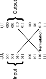
FIG. 1.: Representation of the oracle $U_{f}$ spanning on spins $I_{1}$, $I_{2}$ whose function corresponds to one permutation and results of the query stored on $I_{0}$.

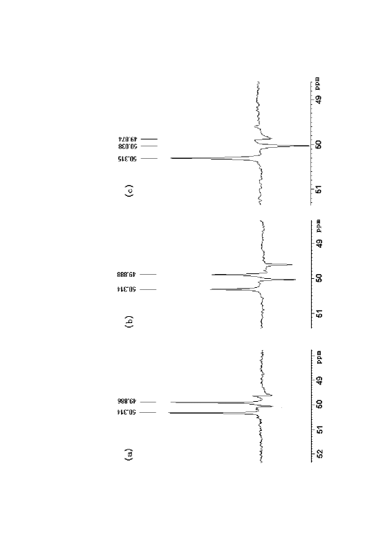
FIG. 2.: Experimental realization of the Brüschweiler’s algorithm using the three spins $1/2$ of ${}^{13}C$ , ${}^{13}C$-labled alanine dissolved in $D_{2}O$. (a) The spectrum of the ancilla qubit in state before the oracle $U_{f}$, two peaks are upword. The shape of the spectrum is used as criterion. (b) The spectrum of the ancilla qubit after the oracle $U_{f}$. The first bit is $1$. (c) The spectrum of the ancilla qubit in the state after the oracle $U_{f}$. The second bit is $0$. The marked state is $10$.

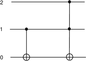
FIG. 3.: Network for realizing the oracle $U_{f}.$

References

- [1] D. Deutsch and R. Josza, Proc. R. Soc. London A., 439, 553(1992).
- [2] P. Shor, in Proceedings of the 35th Annual Symposium on the Foundations of Computer Science, edited by S. Goldwasser(IEEE Computer Society, Los Alamitos) P116.
- [3] L. K. Grover, Phys. Rev. Lett., 79, 325(1997).
- [4] C. Zalka, Phys. Rev. A, 60, 2746(1999).
- [5] D. Abrams and S. Lloyd, Phys. Rev. Lett, 81, 3992(1998).
- [6] R. Brüschweiler, Phys. Rev. Lett., 85, 4815(2000).
- [7] C. Monroe, D. M. Meekhof, and B. E. King, Phys. Rev. Lett., 75, 4714(1995).
- [8] Q. A.Turchette, C. J. Hood, W. Lange, H. Mabuchi, and H. J. Kimble, Phys. Rev. Lett., 75, 4710(1995)
- [9] R. R. Ernst, G. Bodenhausen, and A. Wokaun, “Principles of Nuclear Magnetic Resonance in One and Two Dimensions” (Oxford University Press, 1987)
- [10] D. G. Cory, A. F. Fahmy, and T. F. Havel, Proc. Natl. Acad. Sci. USA, 94, 1634(1997)
- [11] N. A. Gersenfeld and I. L. Chuang, Science, 275, 350(1997)
- [12] J. A. Jones and M. Mosca, J. Chem. Phys., 109, 1648(1998)
- [13] I. L. Chuang, V. L. M. Vandersypen, X. L. Zhou, D. W. Leung & S. Lloyd, Nature, 393, 143(1998)
- [14] J. A. Jones, Prog. Nucl. Mag. Res. Sp., 38, 325 (2001)
- [15] J. A. Jones, Phys. Chem. Comm. 11, 1 (2001)
- [16] G. L. Long, H. Y. Yan, Y. S. Li, C. C. Tu, J. X. Tao, H. M. Chen, M. L. Liu, X. Zhang, J. Luo, L. Xiao, and X. Z. Zeng, Phys. Lett. A, 286, 121(2001).
- [17] S. L. Braunstein, C. M. Caves, R. Josza, N. Linden, S. Popescu, and R. Schack, Phys. Rev. Lett., 83,1054(1999).
- [18] R. Laflamme and D. G. Cory,“NMR quantum information processing and entanglement”, quant-ph/0110029
- [19] W. S. Warren, Science, 277, 1688(1997)
- [20] N. A. Gershenfeld and I. L. Chuang, Science, 277, 1689(1997).
- [21] Z. L. Madi, R.Brüschweiler and R. R. Ernst, J. Chem. Phys., 109, 10603(1998)
- [22] I. L. Chuang, N. Gershenfeld, M. Kubinec, and D. W. Leung, Proc. R. Soc. London A., 454, 447(1998)
- [23] A. Barenco, C. H. Bennett, R. Cleve, D. P. DiVincenzo, N. Margolus, P. Shor, T. Sleator, J. A. Smolin, and H. Weinfurter, Phys. Rev. A, 52, 3457(1995)
- [24] J. A. Jones, R. H. Hansen, and M. Mosca, J. Magn. Res., 135, 353(1998)
- [25] M. Pravia, E. fortunato, Y. Weinstein, M. D. Price, G. Teklemariam, R. J. Nelson, Y. Sharf, S. Somaroo, C. H. Tseng, T. F. Havel, and D. G. Cory, Concepts Magn. Reson.,11, 225 (1999).