Charge in electric field in probability representation

Abstract

Green function and linear integrals of motion for a charged particle moving in electric field are discussed. Wigner function and tomogram of the ststionary states of the charge are obtained. Connection of quantum propagators for Schrödinger evolution equation, Moyal evolution equation and evolution equation in tomographic probability representation for charge moving in electric field is discussed.

1 Introduction

The quantum mechanics formalism is based on the notions of wave function [1, 2, 3, 4, 5] and density matrix [6]. The possible interpretations of quantum properties including the interpretation in terms of hidden variables have been suggested in [7, 8] and analysis of this approach is presented in [9, 10, 11]. The tomographic map [12] gives the possibility to formulate quantum mechanics using the notion of probability and, in principle, avoiding the notion of wave function [13, 14, 15, 16]. The attempts to construct quantum formalism similar to classical one done in the spirit of Moyal approach [17] based on Wigner function [18] were made using quasidistributions of different kind [19, 20, 21, 22]. The evolution equation of such quasidistributions [23, 13] provides the complete information on behaviour of the quantum systems which is equivalent to the information contained in von Neumann equation for density matrix [6]. There are several modern quantum problems [24, 25, 26, 27, 28, 29, 30, 31, 32, 33, 34] related to trapped ions, photons in cavity, quantum computers as well as traditional ones [35, 36] which can be considered in framework of the probability representation of quantum mechanics. In this work we analyse one of these problems for charge moving in electric field.

One of the solvable problems of quantum motion is the problem of charge moving in electric field. It is important problem and we will discuss this problem in framework of tomographic probability representation of quantum states [37, 38, 24, 12, 39, 40, 41, 33, 42].

The probability representation of quantum mechanics was introduced in [13, 14]. The Wigner function [18] of quantum states is the informative characteristic of the state. The optical tomography scheme [24] was used to reconstruct the Wigner function of photons. Extension of the optical tomography method containing two real parameters was suggested in [12]. The tomographic probability distribution of quantum state was employed in [13, 14] to replace the wave function and density matrix by the probability density which determines the state. This approach to description of quantum states created new formalism of quantum mechanics similar to classical statistics. The evolution [13, 14, 43, 16] and energy levels [15, 16] in tomographic representation correspond to Moyal formulation of quantum mechanics [17]. The probability representation was introduced for spin in [44, 45, 46, 47, 48]. The Pauli equation in tomographic representation was obtained in [49]. There are quasidistribution functions which correspond to density matrix in different representations like Wigner function [18], Glauber-Sudarshan $P$-function [19] and [20], Husimi $Q$-function [21]. The tomograms have specific property of standard probability distribution and they completely describe the quantum states. Many physical systems are described by the quadratic Hamiltonians [50]. The charge moving in homogeneous electric field is important example of such systems. The Gaussian and Gauss-Hermite states for such system were studied using time-dependent integrals of motion linear in position and momentum in [51]. The wave functions of Gaussian states and number states can be obtained for the charge moving in electric field in explicit form. The tomographic description of the states is the main goal of our work. We will obtain tomograms and propagator for the evolution equation in the probability representation for the charge moving in electric field. We will also discuss the connection of Green function for Schrödinfer equation and the propagator.

2 Green function and integrals of motion

First we discuss the Green function of Schrödinger evolution equation for the wave function in position representation

$$i\hbar\frac{\partial\psi(x,t)}{\partial t}=\widehat{H}(t)\psi(x,t).$$ (1)

Unitary operator $\widehat{U}(t)$ is called evolution operator of this equation if for any solution $\psi(x,t)$ expressed in terms of the state vector $|\psi,t\rangle$ one has the relation

$$|\psi,t\rangle=\widehat{U}(t)|\psi,0\rangle.$$ (2)

From this equation follows that at the time moment $t=0$ the evolution operator coincides with the identity operator:

$$\widehat{U}(0)=\widehat{1}.$$ (3)

The matrix element of the operator $\widehat{U}(t)$ in position representation is called ”Green function” of the Schrödinger evolution equation (1)

$$G(x,x^{\prime},t)=\langle x|\widehat{U}(t)|x^{\prime}\rangle.$$ (4)

In position representation the equation (2) can be rewritten in the integral form

$$\psi(x,t)=\int G(x,x^{\prime},t)\psi(x^{\prime},0)\,dx^{\prime}.$$ (5)

This equality means that the Green function is the kernel of the evolution operator. It is obvious that for the initial time moment the Green function coincides with Dirac delta-function, i.e.,

$$G(x,x^{\prime},0)=\delta(x-x^{\prime}).$$ (6)

It is easy to obtain the evolution equation for the Green function $G(x,x^{\prime},t)$. Substituting expression (5) into Schrödinger equation for the wave function we get

$$i\hbar\frac{\partial\psi}{\partial t}(x,t)=i\hbar\int\frac{\partial G}{\partial t}(x,x^{\prime},t)\psi(x^{\prime},0)\,dx^{\prime}={\widehat{H}(t)}_{[x]}\psi(x,t)=\int{\widehat{H}(t)}_{[x]}G(x,x^{\prime},t)\psi(x^{\prime},0)\,dx^{\prime},$$ (7)

where notation $\widehat{H}_{[x]}$ means that the energy-operator $\widehat{H}$ acts on the variable $x$ of the Green function. Since the above equations are valid for arbitrary wave function we obtain the following equation for the Green function

$$i\hbar\frac{\partial G}{\partial t}(x,x^{\prime},t)={\widehat{H}(t)}_{[x]}G(x,x^{\prime},t).$$ (8)

Now we discuss the notion of quantum integrals of motion. The operator $\widehat{I}(t)$ is called the integral of motion if its mean does not depend on time, i.e.

$${\left\langle\widehat{I}(t)\right\rangle}_{\psi}=\langle\psi,t|\widehat{I}(t)|\psi,t\rangle$$ (9)

for any solution $|\psi,t\rangle$ of the Schrödinger equation. It means that

$$\frac{d}{dt}{\left\langle\widehat{I}(t)\right\rangle}_{\psi}=\frac{d}{dt}\langle\psi,t|\widehat{I}(t)|\psi,t\rangle=0.$$ (10)

Since the total time derivative can be expressed in the form containing the term with the commutator

$$\frac{d}{dt}{\left\langle\widehat{I}(t)\right\rangle}_{\psi}={\left\langle\frac{\partial\widehat{I}(t)}{\partial t}+\frac{i}{\hbar}[\widehat{H},\widehat{I}(t)]\right\rangle}_{\psi},$$ (11)

the operator $\widehat{I}(t)$ is integral of motion iff it satisfies the evolution equation of the form

$$i\hbar\frac{\partial\widehat{I}(t)}{\partial t}=[\widehat{H},\widehat{I}(t)],$$ (12)

in other words, the operator $\widehat{I}(t)$ is the integral of motion iff its total time derivative is equal to zero:

$$\frac{d\widehat{I}(t)}{dt}=\frac{\partial\widehat{I}(t)}{\partial t}+\frac{i}{\hbar}[\widehat{H},\widehat{I}(t)]=0.$$ (13)

By definition of the evolution operator $\widehat{U}(t)$ one has the equalities

$$|\psi,t\rangle=\widehat{U}(t)|\psi,0\rangle,\qquad\langle\psi,t|=\langle\psi,0|\widehat{U}^{+}(t)=\langle\psi,0|\widehat{U}^{-1}(t).$$ (14)

We used the property of unitarity of the evolution operator which takes place for Hermitian Hamiltonians. By definition of the integral of motion $\widehat{I}(t)$ we have also the equalities

$$\langle\psi,0|\widehat{I}(0)|\psi,0\rangle=\langle\psi,t|\widehat{I}(t)|\psi,t\rangle=\langle\psi,0|\widehat{U}^{-1}(t)\widehat{I}(t)\widehat{U}(t)|\psi,0\rangle,$$ (15)

from which one gets

$$\widehat{I}(0)=\widehat{U}^{-1}(t)\widehat{I}(t)\widehat{U}(t)\quad\text{or}\quad\widehat{I}(t)=\widehat{U}(t)\widehat{I}(0)\widehat{U}^{-1}(t).$$ (16)

This mean that the evolution operator and the integral of motion satisfy the operator equation

$$\widehat{I}(t)\widehat{U}(t)=\widehat{U}(t)\widehat{I}(0).$$ (17)

The matrix elements of the equal operators must be equal, i.e.,

$${\left(\widehat{I}(t)\widehat{U}(t)\right)}_{xx^{\prime}}={\left(\widehat{U}(t)\widehat{I}(0)\right)}_{xx^{\prime}}.$$ (18)

The above equation is written in position representation. Note that for any operator $\widehat{f}$ and function $\psi(x)$ the following equality takes place

$$(\widehat{f}\psi)(x)=\int f(x,x^{\prime})\psi(x^{\prime})\,dx^{\prime},$$ (19)

which is an analog of finite-dimensional equality

$${f(l)}_{i}=\sum\limits^{n}_{j=1}f_{ij}l_{j},$$ (20)

where $f:L\to L$ is linear operator in n-dimensional linear space $L$, $l\in L$ is $n$-vector, $f_{ij}$ and $l_{i}$ are matrix elements of operator $f$ and components of vector $l$, respectively, with respect to some fixed basis of linear space $L$. Equation (18) can be presented in the form

$$\begin{split}\int I(x,y,t)G(y,x^{\prime},t)\,dy&={\widehat{I}(t)}_{[x]}G(x,x^{\prime},t)=\int G(x,y,t)I(y,x^{\prime},0)\,dy=\int I(y,x^{\prime},0)G(x,y,t)\,dy\\ &=\int I^{t}(y,x^{\prime},0)G(x,y,t)\,dy={\widehat{I}^{t}(0)}_{[x^{\prime}]}G(x,x^{\prime},t).\end{split}$$ (21)

Here $\widehat{I}^{t}$ implies the transposed operator. Thus, we obtain system of two equations for Green function in case of physical system with one degree of freedom

$${\widehat{I}(t)}_{[x]}G(x,x^{\prime},t)={\widehat{I}^{t}(0)}_{[x^{\prime}]}G(x,x^{\prime},t),$$ (22)

where the operator $\widehat{I}(t)$ has two components which are independent integrals of motion. This system of equations together with equation (8) and the initial condition (6) provides the complete system of equations determining the Green function. The normalization constant for the Green function can be found using the nonlinear equation for the evolution operator

$$\widehat{U}(t)=\widehat{U}(t-\tau)\widehat{U}(\tau).$$ (23)

This operator equality gives the nonlinear integral equation for the Green function

$$G(x,x^{\prime},t)=\int G(x,y,t-\tau)G(y,x^{\prime},\tau)\,dy.$$ (24)

This equality is equivalent to the initial condition (6) for the Green function.

The considered general properties of the quantum integrals of motion and Green function of Schrödinger evolution equation will be studied for partial quantum system. We consider a particle in a uniform electric filed $F$. The Hamiltonian $\widehat{H}$ of this particle reads

$$\widehat{H}=\frac{\widehat{p}^{2}}{2m}-F\widehat{x}.$$ (25)

If it were the classical particle we would have the trajectory of the particle in the phase space of the form

$$x =x_{0}+\frac{p_{0}}{m}t+\frac{Ft^{2}}{2m},$$ (26)

$$p =p_{0}+Ft$$ (27)

here $x$ is the coordinate and $p$ is the momentum of the classical particle, respectively. Hence, the inverse expressions

$$x_{0} =x-\frac{p}{m}t+\frac{Ft^{2}}{2m},$$ (28)

$$p_{0} =p-Ft$$ (29)

provide the integrals of (classical) motion. It is easy to check that operators

$$\widehat{x}_{0} =\widehat{x}-\frac{\widehat{p}}{m}t+\frac{Ft^{2}}{2m},$$ (30)

$$\widehat{p}_{0} =\widehat{p}-Ft$$ (31)

are integrals of (quantum) motion, i.e. they satisfy the equation (12). These operators are obtained by means of quantization procedure applied to the classical integrals of motion. The physical meaning of the discussed integrals of motion is explained by the fact that these operators describe the initial point in the particle phase space.

For Green function $G(x,x^{\prime},t)$ we have the system of two equations [50]

$$\begin{split}{\widehat{x}_{0}(t)}_{[x]}G(x,x^{\prime},t)&=x^{\prime}G(x,x^{\prime},t),\\ {\widehat{p}_{0}(t)}_{[x]}G(x,x^{\prime},t)&=i\hbar\frac{\partial G}{\partial x^{\prime}}(x,x^{\prime},t),\end{split}$$ (32)

or for the charge moving in electric field

$$\begin{split}\left(x+\frac{i\hbar t}{m}\frac{\partial}{\partial x}+\frac{Ft^{2}}{2m}\right)G(x,x^{\prime},t)&=x^{\prime}G(x,x^{\prime},t),\\ \left(i\hbar\frac{\partial}{\partial x}+Ft\right)G(x,x^{\prime},t)&=-i\hbar\frac{\partial G}{\partial x^{\prime}}(x,x^{\prime},t)\end{split}$$ (33)

with the initial condition (6)

$$G(x,x^{\prime},0)=\delta(x-x^{\prime}).$$ (34)

The system of equations is obtained using the quantum integrals of motion. To solve this system we try to find the Green function in the Gaussian form, i.e.

$$G(x,x^{\prime},t)=N(x^{\prime},t)e^{a(x^{\prime},t)x^{2}+b(x^{\prime},t)x},$$ (35)

where $N(x^{\prime},t)$, $a(x^{\prime},t)$, and $b(x^{\prime},t)$ are unknown functions. Substituting this expression into the first equation of the system (33) we have the equality

$$x+\frac{i\hbar t}{m}\Bigl{(}2a(x^{\prime},t)x+b(x^{\prime},t)\Bigr{)}+\frac{Ft^{2}}{2m}=x^{\prime},$$ (36)

from which we obtain the functions $a(x^{\prime},t)$ and $b(x^{\prime},t)$ in the form

$$a(x^{\prime},t)=\frac{im}{2\hbar t},\qquad b(x^{\prime},t)=-\frac{im}{\hbar t}x^{\prime}+\frac{iFt}{2\hbar}.$$ (37)

To find out the function $N(x^{\prime},t)$ we substitute (35) into the second equation of the system (33). As a result we obtain the equation for this function:

$$\frac{\partial N}{\partial x^{\prime}}=\frac{i}{\hbar}\left(\frac{m}{t}x^{\prime}+\frac{1}{2}Ft\right)N.$$ (38)

To solve this equation we try to find the function $N(x^{\prime},t)$ in the Gaussian form, i.e.,

$$N(x^{\prime},t)=n(t)e^{\alpha(t){x^{\prime}}^{2}+\beta(t)x^{\prime}}.$$ (39)

Substituting this expression into previous equation we obtain the functions $\alpha(t)$ and $\beta(t)$:

$$\alpha(t)=\frac{im}{2\hbar t},\qquad\beta(t)=\frac{iFt}{2\hbar}.$$ (40)

Thus the explicit form of the Green function $G(x,x^{\prime},t)$ reads

$$G(x,x^{\prime},t)=n(t)\exp\Biggl{\{}\frac{im}{2\hbar t}{(x-x^{\prime})}^{2}+\frac{iFt}{2\hbar}(x+x^{\prime})\Biggr{\}},$$ (41)

where the preexponential factor is unknown function of time. To find out the function $n(t)$ we substitute this expression in the equation (8) and get the differential equation of the form

$$\frac{\partial n}{\partial t}=-\left(\frac{1}{2t}+\frac{iF^{2}t^{2}}{8m\hbar}\right)n.$$ (42)

The solution to this equation reads

$$n(t)=\frac{c}{\sqrt{t}}\exp\Biggl{\{}-\frac{iF^{2}t^{3}}{24m\hbar}\Biggr{\}}.$$ (43)

This solution contains unknown constant $c$ and for the Green function we have the explicit expression

$$G(x,x^{\prime},t)=\frac{c}{\sqrt{t}}\exp\Biggl{\{}\frac{im}{2\hbar t}{(x-x^{\prime})}^{2}+\frac{iFt}{2\hbar}(x+x^{\prime})-\frac{iF^{2}t^{3}}{24m\hbar}\Biggr{\}}.$$ (44)

The constant $c$ can be obtained from the nonlinear equation (24). If we substitute the expression (44) into this equation we obtain the equality

$$1=c\sqrt{\frac{2\pi i\hbar}{m}}.$$ (45)

The above equality determines the normalization constant of the Green function

$$c=\sqrt{\frac{m}{2\pi i\hbar}}.$$ (46)

Finally we have the following expression for the Green function

$$G(x,x^{\prime},t)=\sqrt{\frac{m}{2\pi i\hbar t}}\exp\Biggl{\{}\frac{im}{2\hbar t}{(x-x^{\prime})}^{2}+\frac{iFt}{2\hbar}(x+x^{\prime})-\frac{iF^{2}t^{3}}{24m\hbar}\Biggr{\}}.$$ (47)

which has the Gaussian form. The expression in curle brackets is the classical action $S(x,x^{\prime},t)$ multiplied by the factor $i/\hbar$. For $F=0$ we get the Green function for free motion.

The equation for density operator $\widehat{\rho}(t)$ is similar to Schrödinger eqution for the wave function

$$i\hbar\dot{\widehat{\rho}}(t)=[\widehat{H}(t),\widehat{\rho}(t)].$$ (48)

From this equation it is easy to obtain equation for matrix elements of density matrix $\rho(x,x^{\prime},t)=\langle x|\widehat{\rho}(t)|x^{\prime}\rangle$

$$\frac{\partial\rho}{\partial t}(x,x^{\prime},t)+\frac{i}{\hbar}\Bigl{(}{\widehat{H}}_{[x]}\rho(x,x^{\prime},t)-{\widehat{H}^{t}}_{[x^{\prime}]}\rho(x,x^{\prime},t)\Bigr{)}=0.$$ (49)

The Hamiltonian of moving particle with potential $V(x)$ reads

$$\widehat{H}=\frac{\widehat{p}^{2}}{2m}+V(x),$$ (50)

and equation (49) takes the form

$$\frac{\partial\rho}{\partial t}(x,x^{\prime},t)-\Biggl{(}\frac{i\hbar}{2m}\left(\frac{\partial^{2}}{\partial x^{2}}-\frac{\partial^{2}}{\partial{x^{\prime}}^{2}}\right)-\frac{i}{\hbar}\Bigl{(}V(x)-V(x^{\prime})\Bigr{)}\Biggr{)}\rho(x,x^{\prime},t)=0.$$ (51)

The equation for density matrix admits the solutions in factorised form $\psi(x,t)\psi^{*}(x^{\prime},t)$ which describe the pure states of the quantum system.

The Schrödinger equation for stationary state of the particle in the electric field reads

$$\frac{d^{2}\psi}{dx^{2}}+\frac{2m}{\hbar^{2}}\left(\mathcal{E}+Fx\right)\psi=0.$$ (52)

It is well known that for all energy values $\mathcal{E}$ there exists the solution $\psi_{\mathcal{E}}(x)$ of equation (52) given by a formula

$$\psi_{\mathcal{E}}(x)=\frac{{\left(2m\right)}^{1/3}}{\pi^{1/2}F^{1/6}\hbar^{2/3}}\Phi\left(-{\left(\frac{2mF}{\hbar^{2}}\right)}^{1/3}\left(x+\frac{\mathcal{E}}{F}\right)\right),$$ (53)

where $\Phi(x)$ is the Airy function:

$$\Phi(x)=\frac{1}{\sqrt{\pi}}\int\limits^{+\infty}_{0}\cos\left(\frac{u^{3}}{3}+ux\right)\,du=\frac{1}{2\sqrt{\pi}}\int\exp\left\{i\left(\frac{u^{3}}{3}+ux\right)\right\}\,du,$$ (54)

and the coefficient in front of the function $\Phi$ is necessary for normalization of $\psi_{\mathcal{E}}$ to $\delta$-function:

$$\int\psi_{\mathcal{E}}(x)\psi_{\mathcal{E^{\prime}}}(x)\,dx=\delta\left(\mathcal{E^{\prime}}-\mathcal{E}\right).$$ (55)

Plot of the Airy function is presented in Figure (1).

Figure 1: Airy function

Let us introduce notations

$$A=\frac{{\left(2m\right)}^{1/3}}{\pi^{1/2}F^{1/6}\hbar^{2/3}},\quad\alpha=-\left(\frac{2mF}{\hbar^{2}}\right)^{1/3},\quad\varepsilon=\alpha\frac{\mathcal{E}}{F}.$$ (56)

In this notations $\psi_{\mathcal{E}}$ reads $\psi_{\mathcal{E}}(x)=A\Phi\left(\alpha x+\varepsilon\right)$.

3 Weyl representation

The density operator of quantum state can be considered in different reprresentations. One of the representations is Weyl representation. In this representation each operator is described by its symbol. The Weyl symbol of the density operator is called Wigner function.

Now we obtain the equation for the Wigner function. The Wigner function $W(q,p)$ is expressed in terms of matrix elements of density operator as [18]

$$W(q,p)=\int\rho\left(q+\frac{u}{2},q-\frac{u}{2}\right)e^{-\frac{i}{\hbar}pu}\,du.$$ (57)

To obtain the equation for the Wigner function we have to know the correspondence between operators acting on the functions of variables $x$, $x^{\prime}$ and the same operators acting on the functions of variables $q$, $p$. The operators $\widehat{f}_{[x,x^{\prime}]}$ and $\widehat{F}_{[q,p]}$ are called corresponding to each other

$$\widehat{f}_{[x,x^{\prime}]}\longleftrightarrow\widehat{F}_{[q,p]}$$ (58)

if the following equivalent relations are valid for any corresponding to each other density matrix $\rho(x,x^{\prime})$ and the Wigner function $W(q,p)$ of the same quantum state

$$\begin{split}&W(q,p)=\int\rho\left(q+\frac{u}{2},q-\frac{u}{2}\right)e^{-\frac{i}{\hbar}pu}\,du\Rightarrow\\ &\int\left(\widehat{f}_{[x,x^{\prime}]}\rho\right)\left(q+\frac{u}{2},q-\frac{u}{2}\right)e^{-\frac{i}{\hbar}pu}\,du=\left(\widehat{F}_{[q,p]}W\right)(q,p),\end{split}$$ (59)

and

$$\begin{split}&\rho(x,x^{\prime})=\frac{1}{2\pi\hbar}\int W\left(\frac{x+x^{\prime}}{2},p\right)e^{\frac{i}{\hbar}p(x-x^{\prime})}\,dp\Rightarrow\\ &\left(\widehat{f}_{[x,x^{\prime}]}\rho\right)(x,x^{\prime})=\frac{1}{\hbar}\int\left(\widehat{F}_{[q,p]}W\right)\left(\frac{x+x^{\prime}}{2},p\right)e^{\frac{i}{\hbar}p(x-x^{\prime})}\,dp.\end{split}$$ (60)

Now we obtain operators corresponding to the operators $\widehat{x}$, $\widehat{x^{\prime}}$, $\partial/\partial x$, and $\partial/\partial x^{\prime}$.

$$\begin{split}\int\left(\widehat{x}\rho\right)\left(q+\frac{u}{2},q-\frac{u}{2}\right)e^{-\frac{i}{\hbar}pu}\,du&=\int\left(q+\frac{u}{2}\right)\rho\left(q+\frac{u}{2},q-\frac{u}{2}\right)e^{-\frac{i}{\hbar}pu}\,du\\ &=\biggl{(}q+\frac{1}{2}\left(-\frac{\hbar}{i}\frac{\partial}{\partial p}\right)\biggr{)}W(q,p).\end{split}$$ (61)

It means that multiplication of density matrix by the coordinate $x$ provides the action on the Wigner function of the form

$$x\rho(x,x^{\prime})\longleftrightarrow\left(q+\frac{i\hbar}{2}\frac{\partial}{\partial p}\right)W(q,p).$$ (62)

Analogously one can obtain that

$$x^{\prime}\rho(x,x^{\prime})\longleftrightarrow\left(q-\frac{i\hbar}{2}\frac{\partial}{\partial p}\right)W(q,p).$$ (63)

To obtain operators acting on the Wigner function corresponding to operators $\widehat{x}$ and $\widehat{x^{\prime}}$ we used the equation (59). Now to obtain operators acting on the Wigner function corresponding to operators $\partial/\partial x$ and $\partial/\partial x^{\prime}$ acting on the density matrix we use the equation (60) and get

$$\frac{\partial\rho}{\partial x}(x,x^{\prime})=\frac{1}{2\pi\hbar}\int\left(\frac{1}{2}\frac{\partial}{\partial q}+\frac{i}{\hbar}p\right)W\left(\frac{x+x^{\prime}}{2},p\right)e^{\frac{i}{\hbar}p(x-x^{\prime})}\,dp.$$ (64)

By definition of corresponding operators we have

$$\frac{\partial}{\partial x}\rho(x,x^{\prime})\longleftrightarrow\left(\frac{1}{2}\frac{\partial}{\partial q}+\frac{i}{\hbar}p\right)W(q,p),$$ (65)

and analogously

$$\frac{\partial}{\partial x^{\prime}}\rho(x,x^{\prime})\longleftrightarrow\left(\frac{1}{2}\frac{\partial}{\partial q}-\frac{i}{\hbar}p\right)W(q,p).$$ (66)

Now using the obtained correspondence rules and the von Neumenn equation (51) for the density matrix we can write the equation for the Wigner function, which was obtained by Moyal [17]

$$\frac{\partial W}{\partial t}(q,p,t)+\frac{p}{m}\frac{\partial W}{\partial q}(q,p,t)+\frac{i}{\hbar}\Biggl{(}V\left(q+\frac{i\hbar}{2}\frac{\partial}{\partial p}\right)-V\left(q-\frac{i\hbar}{2}\frac{\partial}{\partial p}\right)\Biggr{)}W(q,p,t)=0.$$ (67)

In the case of charged particle moving in electric field the potential energy $V(x)=-Fx$, and one gets the Moyal equation in the form

$$\dot{W}+\frac{p}{m}\frac{\partial W}{\partial q}+\frac{1}{2}F\frac{\partial W}{\partial p}=0.$$ (68)

The Wigner function $W(q,p,t)$ can be found as solution to the Moyal equation. It has the form

$$W(q,p,t)=W_{0}(x_{0},p_{0})$$ (69)

where $W_{0}(q,p)$ is the initial Wigner function and $x_{0}$ and $p_{0}$ are given by equations (28) and (29), respectively. We get

$$W(q,p,t)=W_{0}\left(q-\frac{p}{m}t+\frac{Ft^{2}}{2m},p-Ft\right).$$ (70)

For Wigner function one can introduce the propagator $\Gamma(q,p,q^{\prime},p^{\prime},t)$ of Moyal equation

$$W(q,p,t)=\int\Gamma(q,p,q^{\prime},p^{\prime},t)W(q^{\prime},p^{\prime},0)\,dq^{\prime}\,dp^{\prime}.$$ (71)

In the case of the charge moving in electric field we have explicit expression for the propagator of Moyal equation

$$\Gamma(q,p,q^{\prime},p^{\prime},t)=\delta(x_{0}-q^{\prime})\delta(p_{0}-p^{\prime})=\delta\left(q-\frac{p}{m}t-q^{\prime}+\frac{Ft^{2}}{2m}\right)\delta\left(p-p^{\prime}-Ft\right).$$ (72)

Let us consider example of initial state which is described by the wave function

$$\psi_{0}(x)=\sqrt[4]{\frac{m\omega}{\pi\hbar}}\exp\Biggl{\{}-\frac{m\omega}{2\hbar}x^{2}\Biggr{\}}.$$ (73)

This state can be specially prepared by means of a spring which is removed at the time moment $t=0$. The corresponding Wigner function has the initial form

$$W_{0}(q,p)=2\exp\left\{-\frac{m\omega}{\hbar}q^{2}-\frac{p^{2}}{\hbar m\omega}\right\}.$$ (74)

The evolution of the Wigner function is given by formula

$$\begin{split}W(q,p,t)&=2\exp\Biggl{\{}-\frac{m\omega}{\hbar}q^{2}+\frac{2\omega t}{\hbar}qp-\frac{1}{\hbar m}\left(\omega t^{2}+\frac{1}{\omega}\right)p^{2}-\frac{Ft^{3}\omega}{\hbar m}p\Biggr{.}\\ \Biggl{.}&-\frac{Ft^{2}\omega}{\hbar}q-\frac{F^{2}t^{2}}{\hbar m}\left(\frac{\omega t^{2}}{4}+\frac{1}{\omega}\right)+\frac{2Ft}{\hbar m\omega}\Biggr{\}}.\end{split}$$ (75)

Now we calculate the Wigner’s function of the stationary state of the charged particle with given energy (53). By definition, Wigner function of the state is related to the wave function $\psi_{\mathcal{E}}(x)$ by the formula

$$W_{\mathcal{E}}(q,p)=\int\psi_{\mathcal{E}}\left(q+\frac{u}{2}\right)\psi^{*}_{\mathcal{E}}\left(q-\frac{u}{2}\right)e^{-\frac{i}{\hbar}pu}\,du.$$ (76)

Using expressions (53) and (54) it is easy to show that

$$\begin{split}W_{\mathcal{E}}(q,p)&=\frac{1}{\pi}\sqrt[3]{\frac{m}{F^{2}\hbar^{2}}}\Phi\left(\sqrt[3]{4}\left(\frac{p^{2}}{\alpha^{2}\hbar^{2}}+\alpha q+\varepsilon\right)\right)\\ &=\frac{1}{\pi}\sqrt[3]{\frac{m}{F^{2}\hbar^{2}}}\Phi\left({\left(\frac{1}{mF\hbar}\right)}^{2/3}p^{2}-2{\left(\frac{mF}{\hbar^{2}}\right)}^{1/3}q-2{\left(\frac{m}{F^{2}\hbar^{2}}\right)}^{1/3}\mathcal{E}\right).\end{split}$$ (77)

Plot of the Wigner function is shown in Figure (2).

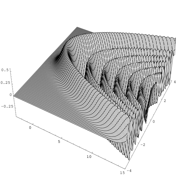
Figure 2: Wigner function

4 Tomographic representation

The tomogram of the quantum state is expressed in terms of Wigner function ($\hbar=1$) [12].

$$w(X,\mu,\nu)=\int W(q,p)e^{ik(X-\mu q-\nu p)}\,\frac{dk\,dq\,dp}{{(2\pi)}^{2}}.$$ (78)

The inverse relation determines the Wigner function in terms of the tomogram

$$W(q,p)=\int w(X,\mu,\nu)e^{i(X-\mu q-\nu p)}\,\frac{dX\,d\mu\,d\nu}{2\pi}.$$ (79)

For pure state described by wave function $\psi(x)$ for tomogram one can obtain the formula in terms of this wave function

$$w(X,\mu,\nu)=\frac{1}{2\pi|\nu|}{\left|\int\psi(y)\exp\left\{\frac{i\mu}{2\nu}y^{2}-\frac{iX}{\nu}y\right\}\,dy\right|}^{2}.$$ (80)

To write the equation for tomogram [14] we have to know the correspondence between operators acting on Wigner functions depending on the variables $q$, $p$ and the same operators acting on the tomograms depending on the variables $X$, $\mu$, $\nu$. Operators $\widehat{F}_{[q,p]}$ and $\widehat{G}_{[X,\mu,\nu]}$ are called corresponding to each other

$$\widehat{F}_{[q,p]}\longleftrightarrow\widehat{G}_{[X,\mu,\nu]}$$ (81)

if the following equivalent relations are valid for any corresponding to each other Wigner function $W(q,p)$ and tomogram $w(X,\mu,\nu)$

$$\begin{split}&w(X,\mu,\nu)=\int W(q,p)e^{-ik(X-\mu q-\nu p)}\,\frac{dk\,dq\,dp}{{(2\pi)}^{2}}\Rightarrow\\ &\int\left(\widehat{F}_{[q,p]}W\right)(q,p)e^{-ik(X-\mu q-\nu p)}\,\frac{dk\,dq\,dp}{{(2\pi)}^{2}}=\left(\widehat{G}_{[X,\mu,\nu]}w\right)(X,\mu,\nu)\end{split}$$ (82)

and

$$\begin{split}&W(q,p)=\int w(X,\mu,\nu)e^{i(X-\mu q-\nu p)}\,\frac{dX\,d\mu\,d\nu}{2\pi}\Rightarrow\\ &\left(\widehat{F}_{[q,p]}W\right)(q,p)=\int\left(\widehat{G}_{[X,\mu,\nu]}w\right)(X,\mu,\nu)e^{i(X-\mu q-\nu p)}\,\frac{dX\,d\mu\,d\nu}{2\pi}.\end{split}$$ (83)

Using the same method which we used for finding the corresponding operators in position and Weyl representation we can get the following relations

$$qW(q,p) \longleftrightarrow-{\left(\frac{\partial}{\partial X}\right)}^{-1}\frac{\partial}{\partial\mu}w(X,\mu,\nu), \qquad\frac{\partial}{\partial q}W(q,p) \longleftrightarrow\mu\frac{\partial}{\partial X}w(X,\mu,\nu),$$ (84)

$$pW(q,p) \longleftrightarrow-{\left(\frac{\partial}{\partial X}\right)}^{-1}\frac{\partial}{\partial\nu}w(X,\mu,\nu), \qquad\frac{\partial}{\partial p}W(q,p) \longleftrightarrow\nu\frac{\partial}{\partial X}w(X,\mu,\nu).$$ (85)

The action of the operators onto homogeneous tomograms must give the homogeneous function. This condition gives the possibility to avoid the ambiguity related with the fact that Wigner function depends on two variables and the tomogram depends on the three variables.

The evolution equation for tomogram in which we reconstruct the Plank constant reads [14]

$$\frac{\partial w}{\partial t}-\mu\frac{\partial w}{\partial\nu}+\frac{i}{\hbar}\Biggl{[}V\left(-{\left(\frac{\partial}{\partial X}\right)}^{-1}\frac{\partial}{\partial\mu}+\frac{i\hbar\nu}{2}\frac{\partial}{\partial X}\right)-V\left(-{\left(\frac{\partial}{\partial X}\right)}^{-1}\frac{\partial}{\partial\mu}-\frac{i\hbar\nu}{2}\frac{\partial}{\partial X}\right)\Biggr{]}w=0.$$ (86)

In our case of charged particle moving in electric field the equation takes the simple form

$$\frac{\partial w}{\partial t}-\mu\frac{\partial w}{\partial\nu}+F\nu\frac{\partial}{\partial X}w=0.$$ (87)

Now we find thetomographic symbols of the integrals of motion. The kernels of the integrals of motion in position representation read

$$\begin{split}x_{0}(x,x^{\prime})&=\left(x+\frac{Ft^{2}}{2m}\right)\delta(x-x^{\prime})-\frac{i\hbar t}{m}\delta^{\prime}(x-x^{\prime}),\\ p_{0}(x,x^{\prime})&=-Ft\delta(x-x^{\prime})+i\hbar\delta^{\prime}(x-x^{\prime}).\end{split}$$ (88)

Using these kernels one can find Weyl symbols of the integrals of motion

$$\begin{split}W_{\widehat{x}_{0}}(q,p)&=\int x_{0}\left(q+\frac{u}{2},q-\frac{u}{2}\right)e^{-\frac{i}{\hbar}pu}\,du=q-\frac{p}{m}t+\frac{Ft^{2}}{2m},\\ W_{\widehat{p}_{0}}(q,p)&=\int p_{0}\left(q+\frac{u}{2},q-\frac{u}{2}\right)e^{-\frac{i}{\hbar}pu}\,du=p-Ft.\end{split}$$ (89)

The tomographic symbols of the integrals of motion are related the their Weyl symbols by the same formulas that the tomogram of a quantum state is related to the Wigner function ($\hbar=1$), i.e.,

$$\begin{split}w_{\widehat{x}_{0}}(X,\mu,\nu)&=\int W_{\widehat{x}_{0}}(q,p)e^{-ik(X-\mu q-\nu p)}\,\frac{dk\,dq\,dp}{{(2\pi)}^{2}}\\ &=\Biggl{(}-{\left(\frac{\partial}{\partial X}\right)}^{-1}\frac{\partial}{\partial\mu}-\frac{t}{m}{\left(\frac{\partial}{\partial X}\right)}^{-1}\frac{\partial}{\partial\nu}+\frac{Ft^{2}}{2m}\Biggr{)}w_{\widehat{1}}(X,\mu,\nu),\\ w_{\widehat{p}_{0}}(X,\mu,\nu)&=\int W_{\widehat{p}_{0}}(q,p)e^{-ik(X-\mu q-\nu p)}\,\frac{dk\,dq\,dp}{{(2\pi)}^{2}}\\ &=-\Biggl{(}{\left(\frac{\partial}{\partial X}\right)}^{-1}\frac{\partial}{\partial\nu}+Ft\Biggr{)}w_{\widehat{1}}(X,\mu,\nu).\end{split}$$ (90)

The tomographic symbol of identity operator in these equalities has the form

$$w_{\widehat{1}}(X,\mu,\nu)=\int\frac{e^{-ikX}}{k^{2}}\,dk\,\delta(\mu)\delta(\nu)$$ (91)

The evolution equation for the tomogram can be solved by means of the Green function (propagator) of this equation relating the initial and current tomograms by the integral transform

$$w(X,\mu,\nu,t)=\int\Pi(X,\mu,\nu,X^{\prime},\mu^{\prime},\nu^{\prime},t)w(X^{\prime},\mu^{\prime},\nu^{\prime},0)\,dX^{\prime}\,d\mu^{\prime}\,d\nu^{\prime}.$$ (92)

The propagator satisfies the evolution equation (we reconstruct the Plank constant)

$$\frac{\partial\Pi}{\partial t}-\mu\frac{\partial\Pi}{\partial\nu}+\frac{i}{\hbar}\Biggl{[}V\left(-{\left(\frac{\partial}{\partial X}\right)}^{-1}\frac{\partial}{\partial\mu}+\frac{i\hbar\nu}{2}\frac{\partial}{\partial X}\right)-V\left(-{\left(\frac{\partial}{\partial X}\right)}^{-1}\frac{\partial}{\partial\mu}-\frac{i\hbar\nu}{2}\frac{\partial}{\partial X}\right)\Biggr{]}\Pi=0,$$ (93)

and the initial condition

$$\Pi(X,\mu,\nu,X^{\prime},\mu^{\prime},\nu^{\prime},0)=\delta(X-X^{\prime})\delta(\mu-\mu^{\prime})\delta(\nu-\nu^{\prime}).$$ (94)

It can be shown [15, 16] that there is the relation of the Green functions of Schrödinger and tomographic evolution equations ($\hbar=1$)

$$\begin{split}\Pi(X,\mu,\nu,X^{\prime},\mu^{\prime},\nu^{\prime},t)&=\frac{1}{4\pi^{2}}\int k^{2}G\left(a+\frac{k\nu}{2},y,t\right)G^{*}\left(a-\frac{k\nu}{2},z,t\right)\delta(y-z-k\nu^{\prime})\\ &\times\exp\biggl{\{}ik\left(X^{\prime}-X+\mu a-\mu^{\prime}\frac{y+z}{2}\right)\biggr{\}}\,dk\,dy\,dz\,da.\end{split}$$ (95)

For the charge moving in the electric field the evolution equation for the propagator reads

$$\frac{\partial\Pi}{\partial t}-\mu\frac{\partial\Pi}{\partial\nu}+F\nu\frac{\partial\Pi}{\partial X}=0.$$ (96)

It has solution

$$\Pi(X,\mu,\nu,X^{\prime},\mu^{\prime},\nu^{\prime},t)=\delta(X-X^{\prime}-Ft)\delta\left(\mu-\mu^{\prime}-\frac{t}{m}\nu\right)\delta(\nu-\nu^{\prime}).$$ (97)

It is interesting to calculate the tomographic probability distribution of stationary state of the charged particle. Evaluating the corresponding integral (80) we get the tomogram of the state

$$w_{\mathcal{E}}\left(X,\mu,\nu\right)=\frac{1}{2\pi|\nu|}{\left|\int\psi_{\mathcal{E}}(y)\exp\left\{\frac{i\mu}{2\hbar\nu}y^{2}-\frac{iX}{\hbar\nu}y\right\}\,dy\right|}^{2}.$$ (98)

Using explicit expressions for $\psi_{\mathcal{E}}$ one can obtain the explicit expression for the tomogram

$$\begin{split}w_{\mathcal{E}}\left(X,\mu,\nu\right)&=\frac{A^{2}\hbar}{4\pi|\mu|}{\left|\Phi\left(\varepsilon-\frac{\alpha X}{\mu}-\frac{\hbar^{2}\alpha^{2}}{4}\frac{\nu^{2}}{\mu^{2}}\right)\right|}^{2}\\ &=\sqrt[3]{\frac{m^{2}}{16\pi^{2}F\hbar}}\frac{1}{|\mu|}{\left|\Phi\left(-{\left(\frac{2m}{F^{2}\hbar^{2}}\right)}^{1/3}\mathcal{E}+{\left(\frac{2mF}{\hbar^{2}}\right)}^{1/3}\frac{X}{\mu}-{\left(\frac{m^{2}F^{2}}{2\hbar}\right)}^{2/3}\frac{\nu^{2}}{\mu^{2}}\right)\right|}^{2}.\end{split}$$ (99)

Plot of the tomogram is shown in Figure (3). One can see the reach structure of the tomogram.

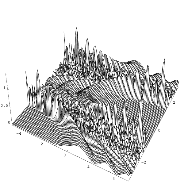
Figure 3: Tomogram

5 Conclusion

Tha main result of our work is the obtaining the tomogram of the stationary state of the charged particle moving in the constant electric field. We found closed connection with integrals of motion, Wigner function and tomograms. The obtained results give a possibility to find new relations for the Airy function.

6 Acknowledgements

This work was supported by the Russian Foundation for Basic Research under Projects Nos. $99$–$02$–$17753$ and $01$–$02$–$17745$. E. V. S thanks Professor T. Seligman for providing a fellowship.

References

• [1] E. Schrödinger, Ann. d. Physik, 79, 489 (1926).
• [2] L. De Broglie, Compt. rend., 183, 447 (1926).
• [3] L. De Broglie, Compt. rend., 184, 273 (1927).
• [4] L. De Broglie, Compt. rend., 185, 380 (1927).
• [5] E. Madelung, Zeits. f. Physik, 40, 332 (1926).
• [6] J. von Neumann, Mathematische Grundlagen der Quantenmechanik. Springer, Berlin, 1932.
• [7] D. Bohm, Phys. Rev., 85, 166 (1952).
• [8] D. Bohm, Phys. Rev., 85, 180 (1952).
• [9] J. S. Bell, Speakable and Unspeakable in Quantum Mechanics. Cambridge University Press, Cambridge, 1987.
• [10] Ya. P. Terletskii and A. A. Gusev, Problems of Causality in Quantum Mechanics. Inostrannaya Literatura, Moscow, 1955.
• [11] J. A. Wheeler and W. H. Zurek (eds.), Quantum Theory and Measurement. Princeton University Press, Princeton, 1983.
• [12] S. Mancini, V. I. Man’ko, and P. Tombesi, Quantum Semiclass. Opt., 7, 615 (1995).
• [13] S. Mancini, V. I. Man’ko, and P. Tombesi, Found. Phys., 27, 801 (1997).
• [14] S. Mancini, V. I. Man’ko, and P. Tombesi, Phys. Lett. A, 213, 1 (1996).
• [15] O. V. Man’ko and V. I. Man’ko, J. Russ. Laser Research, 18, 407 (1997).
• [16] V. I. Man’ko, J. Russ. Laser Research, 17, 579 (1996).
• [17] J. E. Moyal, Proc. Cambridge Philos. Soc., 45, 99 (1949).
• [18] W. Wigner, Phys. Rev., 40, 749 (1932).
• [19] R. J. Glauber, Phys. Rev. Lett., 10, 84 (1963).
• [20] E. C. G. Sudarshan, Phys. Rev. Lett., 10, 277 (1963).
• [21] K. Husimi, Proc. Phys. Math. Soc. Jpn., 23, 264 (1940).
• [22] J. M. Gracia-Bondía and J. C. Várilly, Ann. Phys., 190, 107 (1989).
• [23] C. Brif and A. Mann, Phys. Rev. A, 59, 971 (1999).
• [24] D. T. Smithey, M. Beck, M. G. Raymer, and A. Faridani, Phys. Rev. Lett., 70, 1244 (1993).
• [25] M. M. Nieto, Phys. Lett. A, 219, 180 (1996).
• [26] D. M. Meekhof, G. Monroe, B. E. King, W. M. Itano, and D. Wineland, Phys. Rev. Lett., 76, 1796 (1996).
• [27] S. Haroche, Nuovo Cimento B, 110, 545 (1995).
• [28] O. V. Man’ko, Phys. Lett. A, 228, 29 (1997).
• [29] V. I. Man’ko and A. Wünsche, Quantum Semiclass. Opt., 9, 381 (1997).
• [30] P. J. Bardroff, C. Leichte, G. Schrade, and W. P. Schleich, Phys. Rev. Lett., 77, 2198 (1996).
• [31] R. L. de Matos Filho and W. Vogel, Phys. Rev. A, 54, 4560 (1996).
• [32] S. Wallentowitz and W. Vogel, Phys. Rev. A, 53, 4528 (1996).
• [33] K. Banaszek and K. Wodkiewicz, Phys. Rev. Lett., 76, 4344 (1996).
• [34] Pieter Kok and Samuel L Braunstein, J. Phys. A, 34, 6185 (2001).
• [35] G. Cristofano, D. Giuliano, and G. Maiella, J. Phys. I France, 6, 7, 861 (1996).
• [36] L. D. Landau, Z. Physik, 45, 430 (1927).
• [37] J. Bertrand and P. Bertrand, Found. Phys., 17, 397 (1987).
• [38] K. Vogel and H. Risken, Phys. Rev. A, 40, 2847 (1989).
• [39] G. M. D’Ariano, S. Mancini, V. I. Man’ko, and P. Tombesi, Quantum Semiclass. Opt., 8, 1017 (1996).
• [40] U. Leonhardt, Phys. Rev. A, 53, 2998 (1996).
• [41] S. Mancini, V. I. Man’ko, and P. Tombesi, Europhys. Lett., 37, 79 (1997).
• [42] S. Mancini, V. I. Man’ko, and P. Tombesi, J. Mod. Opt, 44, 2281 (1997).
• [43] V. I. Man’ko, M. Moshinsky, and A. Sharma, Phys. Rev. A, 59, 1809 (1999).
• [44] V. V. Dodonov and V. I. Man’ko, Phys. Lett. A, 229, 335 (1997).
• [45] O. V. Man’ko and V. I. Man’ko, Zh. Éksp. Teor. Fiz, 112, 796 (1997).
• [46] V. A. Andreev and V. I. Man’ko, JETP, 114, 437 (1998).
• [47] G. S. Agarwal, Phys. Rev. A, 57, 671 (1998).
• [48] S. Weigert, Phys. Rev. Lett., 84, 802 (2000).
• [49] S. Mancini, O. V. Man’ko, V. I. Man’ko, and P. Tombesi, J. Phys. A, 34, 3461 (2001).
• [50] I. A. Malkin and V. I. Man’ko, Dynamical Symmetries and Coherent States of Quantum Systems. Nauka, Moscow, 1979. [in Russian];
V. V. Dodonov and V. I. Manko,
Invariants and Evolution of Nonstationary Quantum Systems. Proceedings of the Lebedev Physics Institute, vol. 183. (Edited by M. A. Markov) (Nova Science, Commack, 1989).
• [51] I. A. Malkin, V. I. Man’ko, and D. A. Trifonov, Phys. Lett. A, 30, 414 (1969);
I. A. Malkin, V. I. Man’ko, and D. A. Trifonov,
Phys. Rev. D, 2, 1371 (1970);
I. A. Malkin, V. I. Man’ko, and D. A. Trifonov,
J. Math. Phys., 14, 576 (1973).