Scalar charged particle in Weyl–Wigner–Moyal phase space.
Constant magnetic field

Abstract

A relativistic phase-space representation for a class of observables with matrix-valued Weyl symbols proportional to the identity matrix (charge-invariant observables) is proposed. We take into account the nontrivial charge structure of the position and momentum operators. The evolution equation coincides with its analog in relativistic quantum mechanics with nonlocal Hamiltonian under conditions where particle-pair creation does not take place (free particle and constant magnetic field). The differences in the equations are connected with peculiarities of the constraints on the initial conditions. An effective increase in coherence between eigenstates of the Hamiltonian is found and possibilities of its experimental observation are discussed.

1 Introduction

In this paper, we continue our previous study [1] of the phase-space representation for relativistic quantum mechanics. We have established two problems in developing the Weyl–Wigner–Moyal (WWM) formalism for the relativistic case. First of all, it is worth noting that Weyl transformation does not include time as a dynamical variable, i.e., it is not Lorentz invariant. The second problem relates to the existence of a charge variable, which is a specific degree of freedom in relativistic quantum mechanics [2]. This degree of freedom appears due to the procedure of canonical quantization of the relativistic particle [3]; the presence of this degree of freedom results in the fact that the standard position operator is not well defined [2, 4, 5, 6]. Therefore, we points out the nontrivial charge structure of the position operator here. In the context of the phase-space quantization, this problem is still open.

Nowadays, different approaches to solve these problems are well known. Each of them has at least two alternative solutions with different interpretations. In short, we emphasize approaches where the problem of Lorentz invariance is solved by the generalization of Weyl transformation over the whole space–time (stochastic interpretation of quantum mechanics, de Groot–van Leeuwen–van Weert’s approach [7]), and those ones where Weyl transformation is applied in the three-dimensional space or on a space-like hyper-surface. The second problem can be solved in two ways — using either the standard position operator or Newton–Wigner position operator [4]. A list of references on the problem can be found in our previous work [1]; here we would like to complete the list.

The relativistic Wigner function for spin-1/2 particles in magnetic field was introduced in [8]. This approach was realized using the standard (three-dimensional) Weyl transformation and Dirac equation; therefore, one can say, that the standard position operator was used.

The consideration based on Weyl transformation in the three-dimensional space was considered in [9] for the semirelativistic approximation.

The Wigner function for the covariant harmonic oscillator and for the light waves was treated in [10]; while in [11] it was shown, that space–time geometry of relativistic particles corresponds to the four-dimensional phase space of the coupled oscillators, and the corresponding Wigner function was presented.

In our consideration [1] of a spin-0 free particle, we used the following assumptions:

1. Weyl transformation in the six-dimensional phase space (related to the three-dimensional configuration space) or, more generally, on the spacelike hypersurface in the context of Tomonaga–Schwinger approach to quantum field theory [12], is considered;

2. The standard position operator instead of Newton–Wigner position operator is used.

The argumentation in favor of (i) follows. The mean values calculated in this approach coincide with those calculated in the usual (Schrödinger) representation, which is Lorentz invariant. The three-dimensional integration is a consequence of the fact, that the scalar product of states in the Schrödinger representation is determined on a space-like hyper-surface. It cannot be redefined in the whole space–time domain without additional physical assumptions. Furthermore, it is worth noting that this approach can be explained within the framework of the concept of a reference frame in which a reduction of the quantum state takes place (for a details and review of recent experiments see [13]).

The argumentation in favor of (ii) is the fact that the approach using the Newton–Wigner position operator is not Lorentz invariant even in the Schrödinger representation. Here one faces more difficult problems concerning the definition of mean values and the wave equation itself. On the other hand, using the standard position operator enables one to define the probability density for localized states in the domain of the positive (negative) energy [14].

We have considered spin-0 particles using the Feshbach–Villars formalism [2] and restricted ourselves by the class of observables for which their matrix-valued Weyl symbols are proportional to the identity matrix (charge-invariant observables).

The aim of the paper is to generalize this approach to a particle in a static magnetic field. This case, like the free particle case, admits of the one-particle interpretation of relativistic quantum mechanics. We pay special attention to the problem of the influence of the nontrivial charge structure of the position (and momentum) operator on the mean values of the charge-invariant observables.

Contrary to the free particle case, not only the position operator but the momentum operator as well have the nontrivial charge structure [15]. The generalization of the Newton–Wigner position operator approach is the theory with a nonlocal Hamiltonian [16]

$$\hat{E}=\sqrt{m^{2}c^{4}+c^{2}\left[\hat{p}-eA\left(\hat{q}\right)\right]^{2}};$$ (1)

here we call it the nonlocal theory. It is worth noting, that term “nonlocal” has several meanings in modern quantum physics. We use it here for pointing out the fact, that differential equations contain derivatives up to infinite order.

Contrary to the case of nonstationary electromagnetic field, the Hamiltonian (1) can be redefined by extending its action on the charge domain of the Hilbert space

$$\hat{H}^{nl}=\tau_{3}\hat{E}$$ (2)

and it can be considered as the Hamiltonian of the standard theory

$$\hat{H}=\left(\tau_{3}+i\tau_{2}\right)\frac{\left(\hat{p}-eA\left(\hat{q}\right)\right)^{2}}{2m}+\tau_{3}mc^{2}$$ (3)

in a particular representation that we call the nonlocal theory representation. Here and bellow $\tau_{i}$ are the 2$\times$2 matrices defined in [2]. Generally speaking, the operators $\hat{p}$ and $\hat{q}$ from (1) differ from the standard momentum and position operators, which are employed in (3). Therefore, we call $\hat{p}$ and $\hat{q}$ from (1) the momentum and position operators of nonlocal theory. Contrary to the free particle case, these operators are not even parts of the standard position and momentum operators. If $A\left(\hat{q}\right)=0$, i.e., in the absence of magnetic field, expression (2) is the Hamiltonian of free particle in the Newton–Wigner position operator representation.

In Section 2 we consider the general properties of algebra of charge-invariant observables. In Section 3 we introduce the four-component (related to a particle, anti-particle and two interference components) Wigner function for charge-invariant observables and consider its evolution equation. The Heisenberg picture of motion and an extension of the concept of Weyl symbol for charge-invariant observables, which in our approach contains four components, are given in Section 4. Section 5 is devoted to the consideration of specific constraints on the Wigner function for charge-invariant observables, which is a basic difference between the standard and nonlocal theories. This peculiarity has a simple physical sense and is responsible for an effective increase in coherence between eigenstates of the Hamiltonian; this is considered in Section 6 along with simple examples and a proposal of the possibility of experimental observation.

2 Charge-invariant observables

For a consistent development of the WWM formalism, one should define Weyl transformation. Following [1] we describe an operator $\hat{A}$ by the 2$\times$2 operator-valued matrix $\hat{A}_{\alpha}{}^{\beta}$, and the corresponding matrix-valued Weyl symbol by $c$-number matrix $A_{\alpha}{}^{\beta}(p,q)$. The Greek indices take values $\pm 1$ and, whenever possible, we will label them as $\pm$. Since the Hilbert space of states for scalar charged particles has an indefinite metric, one should distinguish between covariant and contravariant indices. Taking the above mentioned into account, one can write the Weyl transformation as follows

$$\hat{A}_{\alpha}{}^{\beta}=\sum_{\gamma=\pm 1}\int\limits_{-\infty}^{+\infty}A_{\gamma}{}^{\beta}\left(p,q\right)\hat{W}_{\alpha}{}^{\gamma}\left(p,q\right)dp\,dq,$$ (4)

where $\hat{W}_{\alpha}{}^{\beta}\left(p,q\right)$ is the operator of quasiprobability density.

Let us introduce the momentum (or position) part of the eigenfunction of the Hamiltonian (3) as the solution of the following eigenvalue problem:

$$\frac{1}{2m}\left(\hat{p}-eA\left(\hat{q}\right)\right)^{2}\varphi_{n}\left(p\right)=e(n)\varphi_{n}\left(p\right),$$ (5)

where $n$ is a set of quantum numbers. The eigenvalue modulus of Hamiltonians (1)–(3) can be expressed through $e(n)$

$$E(n)=mc^{2}\sqrt{1+\frac{2}{mc^{2}}e(n)}.$$ (6)

In the representation of these functions, Weyl transformation (4) has the following form:

$$A_{nm;\alpha}{}^{\beta}=\int\limits_{-\infty}^{+\infty}A_{\alpha}{}^{\beta}\left(p,q\right)W_{nm}\left(p,q\right)dp\,dq$$ (7)

where $W_{nm}\left(p,q\right)$ is the Hermitian generalization of the Wigner function [17, 18]

$$W_{nm}(p,q)=\frac{1}{{(2\pi\hbar)^{d}}}\int\limits_{-\infty}^{+\infty}{\varphi_{m}^{*}\left({p+\frac{P}{2}}\right)\varphi_{n}\left({p-\frac{P}{2}}\right)\exp\left(-\frac{i}{\hbar}Pq\right)dP}$$ (8)

with $d$ being the dimensionality of the configuration space. The final transformation to the energy representation, where the matrix of the Hamiltonian (3) has a diagonal form, is realized by the following transformation matrix:

$$U_{nm;\alpha}{}^{\beta}=\frac{1}{2\sqrt{mc^{2}E(n)}}\left[\left(E(n)+mc^{2}\right)\delta_{\alpha}{}^{\beta}+\left(E(n)-mc^{2}\right)\tau_{1;\alpha}{}^{\beta}\right]\delta_{nm}.$$ (9)

Following [1] we restrict ourselves to observables in which the matrix-valued Weyl symbols are proportional to the identity matrix

$$A_{\alpha}{}^{\beta}(p,q)=A(p,q)\delta_{\alpha}{}^{\beta}$$ (10)

and call the class of dynamical variables, which corresponds to such symbols, the class of charge-invariant observables. It is worth noting that the Hamiltonian and current do not belong to this class. However, in Section 3 we present a symbol that plays the role of the Hamiltonian in our consideration.

The Weyl transformation for charge-invariant observables in the energy representation has the form

$$A^{E}{}_{nm;\alpha}{}^{\beta}=R_{\alpha}{}^{\beta}(m,n)\int\limits_{-\infty}^{+\infty}{A(p,q)W_{nm}(p,q)dp\,dq},$$ (11)

where $A^{E}{}_{nm;\alpha}{}^{\beta}$ is the operator matrix of a charge-invariant observable in the energy representation. Contrary to nonlocal theory and the nonrelativistic case, there is a matrix-valued function $R_{\alpha}{}^{\beta}(m,n)$

$$R_{\alpha}{}^{\beta}(m,n)=\sum_{l,k=0}^{\infty}\sum_{\gamma=\pm 1}U_{lm;\gamma}{}^{\beta}U^{-1}_{nk;\alpha}{}^{\gamma}=\varepsilon(m,n)\delta_{\alpha}{}^{\beta}+\chi(m,n)\tau_{1;\alpha}{}^{\beta}$$ (12)

with even and odd parts expressed through the energy spectrum (6) as follows:

$$\varepsilon(m,n)=\frac{{E(m)+E(n)}}{{2\sqrt{E(m)E(n)}}},$$ (13)

$$\chi(m,n)=\frac{{E(m)-E(n)}}{{2\sqrt{E(m)E(n)}}}.$$ (14)

Functions $\varepsilon(m,n)$ and $\chi(m,n)$ play a crucial role in our consideration. We call them the $\varepsilon$- and $\chi$-factors.

The expressions for even $[\hat{A}]$ and odd $\{\hat{A}\}$ parts of the operator of a charge-invariant observable in terms of its Weyl symbol follow from (11)

$$\left[{A^{E}}\right]_{nm;\alpha}{}^{\beta}=\varepsilon(m,n)\delta_{\alpha}{}^{\beta}\int\limits_{-\infty}^{+\infty}{A(p,q)W_{nm}(p,q)dp\,dq}$$ (15)

$$\left\{{A^{E}}\right\}_{nm;\alpha}{}^{\beta}=\chi(m,n)\tau_{1;\alpha}{}^{\beta}\int\limits_{-\infty}^{+\infty}{A(p,q)W_{nm}(p,q)dp\,dq}.$$ (16)

One can obtain the inverse formulas connecting Weyl symbols with the operator, and its even and odd parts

$$A(p,q)\delta_{\alpha}{}^{\beta}=(2\pi\hbar)^{d}\sum_{\gamma=\pm 1}\sum_{m,n=0}^{\infty}{R^{-1}{}_{\gamma}{}^{\beta}(m,n)A^{E}{}_{nm;\alpha}{}^{\gamma}W_{mn}(p,q)},$$ (17)

$$A(p,q)\delta_{\alpha}{}^{\beta}=(2\pi\hbar)^{d}\sum_{mn}{\varepsilon^{-1}(m,n)\left[{A^{E}}\right]_{nm;\alpha}{}^{\beta}W_{mn}(p,q)},$$ (18)

$$A(p,q)\delta_{\alpha}{}^{\beta}=(2\pi\hbar)^{d}\sum_{\gamma=\pm 1}\sum_{m,n=0}^{\infty}{\chi^{-1}(m,n)\tau_{1\gamma}{}^{\beta}\left\{{A^{E}}\right\}_{nm;\alpha}{}^{\gamma}W_{mn}(p,q)}.$$ (19)

Comparing (18) and (19) we conclude that matrix elements of even and odd parts of the operator of an arbitrary charge-invariant observable are uniquely related to each other

$$\{A^{E}\}_{nm;\alpha}{}^{\beta}=\frac{{E(m)-E(n)}}{{E(m)+E(n)}}\sum_{\gamma=\pm 1}{\tau_{1;\gamma}{}^{\beta}[A^{E}]_{nm;\alpha}{}^{\gamma}}.$$ (20)

Now we consider the expression for the time derivative of a charge-invariant observable through its Weyl symbol as was done in [1]. To do this, one should use the Heisenberg equation

$$\partial_{t}\hat{A}=\frac{1}{i\hbar}\left[\hat{A},\hat{H}\right].$$ (21)

The commutator can be written in the form of Weyl transform of the matrix-valued Moyal bracket (see [1]). Equation (21) in the energy representation can be written as follows

$$\partial_{t}A^{E}_{nm;\alpha}{}^{\beta}=\int\limits_{-\infty}^{+\infty}\left\{A(p,q),G_{\alpha}{}^{\beta}\left(m,\{p,q\},n\right)\right\}_{M}W_{nm}(p,q)dp\,dq$$ (22)

where the notation

$$G_{\alpha}{}^{\beta}\left(m,\{p,q\},n\right)=\frac{E^{\star 2}(p,q)}{2\sqrt{E(m)E(n)}}\left(\tau_{3;\alpha}{}^{\beta}+i\tau_{2;\alpha}{}^{\beta}\right)$$ (23)

$$E^{\star 2}(p,q)=m^{2}c^{4}+c^{2}\Big{(}p-eA\left(q\right)\Big{)}^{2}$$ (24)

is introduced.

The Moyal bracket is defined in such a way to provide coincidence with the Poisson bracket at $\hbar\rightarrow 0$, namely,

$$\left\{A(p,q),B(p,q)\right\}_{M} =\frac{1}{i\hbar}\left(A(p,q)\star B(p,q)-B(p,q)\star A(p,q)\right)$$ (25)

$$=\frac{2}{\hbar}A(p,q)\sin\left\{\frac{\hbar}{2}\left(\overleftarrow{\partial_{q}}\overrightarrow{\partial_{p}}-\overleftarrow{\partial_{p}}\overrightarrow{\partial_{q}}\right)\right\}B(p,q)$$

where the Moyal star-product is determined as usually

$$\star\equiv\exp\left\{\frac{i\hbar}{2}\left(\overleftarrow{\partial_{q}}\overrightarrow{\partial_{p}}-\overleftarrow{\partial_{p}}\overrightarrow{\partial_{q}}\right)\right\}.$$ (26)

Contrary to the free particle case [1], expression (22) does not have a classical form even if $A(p,q)$ is a linear function of $p$ and $q$. The semiclassical approximation in static magnetic field for the standard theory has a more complicated structure than that used in nonlocal theory. In Section 4 we consider another approach to the Heisenberg picture of motion and show that these peculiarities are related to the form of the Wigner function only and do not change the equation of motion.

3 Wigner function and quantum Liouville equation for charge-invariant observables

In order to find the explicit form of the Wigner function for charge-invariant observables, we start with the expression for means. Let $C_{n;\alpha}$ be the wave function in the energy representation (the decomposition coefficient of the wave function presented in the form of series in eigenstates of the Hamiltonian (3)). Thus the mean of the charge-invariant observable $\hat{A}$ is written in the explicit form

$$\overline{A}=\sum_{\alpha,\beta=\pm 1}\sum_{m,n=0}^{\infty}C_{m;\beta}^{*}C_{n;}{}^{\alpha}A^{E}_{nm;\alpha}{}^{\beta}.$$ (27)

Substituting (11) in (27), one can obtain for the mean

$$\overline{A}=\int\limits_{-\infty}^{+\infty}A(p,q)W(p,q)dp\,dq,$$ (28)

where the Wigner function for charge-invariant observable can be presented as the sum of four terms

$$W(p,q)=\sum_{\alpha=\pm 1}\left(W_{[\alpha]}(p,q)+W_{\{\alpha\}}(p,q)\right).$$ (29)

This approach has been applied to construct the covariant Wigner function in [7]. We call $W_{[\pm]}(p,q)$ the even part of the Wigner function. It can be written as follows

$$W_{[\pm]}(p,q)=\sum_{n,m=0}^{\infty}{\varepsilon(m,n)}W_{nm}(p,q)C_{m;}^{*}{}_{\pm}C_{n;}{}^{\pm}.$$ (30)

In a similar way, we call $W_{\{\pm\}}(p,q)$ the odd part of the Wigner function defined as

$$W_{\{\pm\}}(p,q)=\sum_{n,m=0}^{\infty}{\chi(m,n)}W_{nm}(p,q)C_{m;}^{*}{}_{\pm}C_{n;}{}^{\mp}.$$ (31)

Note that here use other symbols for the even and odd parts of the Wigner function than those employed in [1].

The Wigner function for charge-invariant observables can be defined in an alternative way. To do this, we consider the wave function in the nonlocal theory representation

$$\psi_{\pm}(p)=\sum_{n=0}^{\infty}C_{n;\pm}\varphi_{n}(p).$$ (32)

Now one can write the components of the Wigner function as follows

$$W_{[\pm]}(p,q)\!=\!\frac{1}{{(2\pi\hbar)^{d}}}\!\int\limits_{-\infty}^{+\infty}\!{\varepsilon\!\left(\!p\!+\!\frac{P}{2}\!,\!p_{1}\!;\!p\!-\!\frac{P}{2}\!,\!p_{2}\!\right)\!\psi_{\pm}^{*}\!(p_{1})\!\psi^{\pm}\!(p_{2})\!e^{-\frac{i}{\hbar}Pq}\!d\!P\,d\!p_{1}\,d\!p_{2}}\!,$$

(33)

$$W_{\{\pm\}}(p,q)\!=\!\frac{1}{{(2\pi\hbar)^{d}}}\!\int\limits_{-\infty}^{+\infty}\!{\chi\!\left(\!p\!+\!\frac{P}{2}\!,\!p_{1}\!;\!p\!-\!\frac{P}{2}\!,\!p_{2}\!\right)\!\psi_{\pm}^{*}\!(p_{1})\!\psi^{\mp}\!(p_{2})\!e^{-\frac{i}{\hbar}Pq}\!d\!P\,d\!p_{1}\,d\!p_{2}}\!,$$

(34)

where the following generalized functions are introduced:

$$\varepsilon(p^{\prime},p_{1};p^{\prime\prime},p_{2})=\sum_{n,m=0}^{\infty}{\varepsilon(m,n)\varphi_{m}^{*}(p^{\prime})\varphi_{m}(p_{1})\varphi_{n}(p^{\prime\prime})\varphi_{n}^{*}(p_{2})}$$ (35)

$$\chi(p^{\prime},p_{1};p^{\prime\prime},p_{2})=\sum_{n,m=0}^{\infty}{\chi(m,n)\varphi_{m}^{*}(p^{\prime})\varphi_{m}(p_{1})\varphi_{n}(p^{\prime\prime})\varphi_{n}^{*}(p_{2})}.$$ (36)

Following [1] we obtain the evolution equation for each component separately. To do this, we differentiate expressions (30) and (31) with respect to time and substitute the time derivatives from the Klein–Gordon equation in the energy representation

$$i\hbar\partial_{t}C_{n;\alpha}=E(n)\sum_{\beta=\pm 1}\tau_{3;}{}^{\beta}{}_{\alpha}C_{n;\beta}.$$ (37)

In view of the star-eigenvalue equations [19]

$$E(p,q)\star W_{nm}(p,q)=E(n)W_{nm}(p,q)$$

$$W_{nm}(p,q)\star E(p,q)=E(m)W_{nm}(p,q)$$ (38)

we obtain the quantum Liouville equation in the following form:

$$\partial_{t}W_{[\pm]}(p,q,t)=\pm\left\{E(p,q),W_{[\pm]}(p,q,t)\right\}_{M}$$ (39)

$$\partial_{t}W_{\{\pm\}}(p,q,t)=\mp\left[E(p,q),W_{\{\pm\}}(p,q,t)\right]_{M}.$$ (40)

The Moyal bracket in (39) is defined by expressions (25). Furthermore, we have used the anti-Moyal bracket in (40), which is defined as follows

$$\left[A(p,q),B(p,q)\right]_{M} =\frac{1}{i\hbar}\Big{(}A(p,q)\star B(p,q)+B(p,q)\star A(p,q)\Big{)}$$ (41)

$$=\frac{2}{i\hbar}A(p,q)\cos\left\{\frac{\hbar}{2}\left(\overleftarrow{\partial_{q}}\overrightarrow{\partial_{p}}-\overleftarrow{\partial_{p}}\overrightarrow{\partial_{q}}\right)\right\}B(p,q).$$

In these formulas,$E(p,q)$ plays the role of the Hamiltonian; it is determined as ‘the star square root’ of expression (24)

$$E(p,q)=\sqrt[\star]{{m^{2}c^{4}+c^{2}[p-eA(q)]^{2}}}.$$ (42)

This is fairly unexpected, since in nonrelativistic quantum mechanics a classical variable is mapped onto the corresponding Weyl symbol (at least, in the Schrödinger picture of motion or at the initial time moment in the Heisenberg picture). The classical Hamilton function differs from (42) since it employs the square root instead of the star square root. It gives different pictures of the classical and quantum evolutions.

In the Appendix, we consider an approximate expression for the relativistic rotator (simplified model of the particle motion in a homogeneous magnetic field). From this example, one can see that the star square root results in the appearance of independent power series expansion in the cyclotron frequency together with the expansion in position and momentum (93). The cyclotron frequency is inversely proportional to the square of the characteristic oscillator length, which corresponds, in many cases, to the wave packet width. Therefore, one can say, that the star square root introduced results in specific effects which appear in strong magnetic field and for very strong localization (of the order of the Compton wavelength).

It is worth noting that such behaviour of the relativistic system does not relate to the nontrivial charge structure of position and momentum operators because equation (39) with Hamiltonian (42) are valid for nonlocal theory as well.

Consider the odd part of the Wigner function (31), (34). It was mentioned in [7], that it is not important for macroscopic values. Indeed, the existence of states, where this part of the Wigner function is not equal to zero contradicts to charge superselection rule [20]. Such a state is equivalent to the superposition of states with different charge signs. According to the contemporary concept, if such state appears as a result of the physical process, the superposition is reduced to the mixed state, which results in the creation of particle pairs [21]. In our representation, this means that the odd part of the Wigner function becomes zero. However, it appears when an external electric or nonstatic field is applied. Therefore, we take into account its existence here.

The solutions of the system of equations (39) and (40) are not independent. There exists a specific constraint on them. To find it, one should take the Fourier transform and make the standard change of variables in each component of (33), (34). Similar to the free particle case [1], we obtain four expressions where on the left-hand side there are products of two wave functions of different arguments, and on the right-hand side we obtain integral expressions dependent on the Wigner function components. Splitting them into pairs and equating the resulting expressions, due to the equality of their left-hand sides, we obtain the constraint we are looking for:

$$\int\limits_{-\infty}^{+\infty}{\varepsilon^{-1}(p_{1},p^{\prime};p_{2},p^{\prime\prime})W_{[+]}\left(\frac{1}{2}(p_{1}+p_{2}),q_{1}\right)e^{\frac{i}{\hbar}(p_{1}-p_{2})q}dp_{1}\,dp_{2}}\,dq$$

$$\times\int\limits_{-\infty}^{+\infty}{\varepsilon^{-1}(p_{1},p^{\prime};p_{2},p^{\prime\prime})W_{[-]}\left(\frac{1}{2}(p_{1}+p_{2}),q_{2}\right)e^{\frac{i}{\hbar}(p_{1}-p_{2})q}dp_{1}\,dp_{2}\,dq}$$

$$=\int\limits_{-\infty}^{+\infty}{\chi^{-1}(p_{1},p^{\prime};p_{2},p^{\prime\prime})W_{\{+\}}\left(\frac{1}{2}(p_{1}+p_{2}),q_{1}\right)e^{\frac{i}{\hbar}(p_{1}-p_{2})q}dp_{1}\,dp_{2}}\,dq$$

$$\times\int\limits_{-\infty}^{+\infty}{\chi^{-1}(p_{1},p^{\prime};p_{2},p^{\prime\prime})W_{\{-\}}\left(\frac{1}{2}(p_{1}+p_{2}),q_{2}\right)e^{\frac{i}{\hbar}(p_{1}-p_{2})q}dp_{1}\,dp_{2}\,dq},$$

(43)

where the following generalized functions are introduced:

$$\varepsilon^{-1}(p_{1},p^{\prime};p_{2},p^{\prime\prime})=\sum_{n,m=0}^{\infty}{\varepsilon^{-1}(m,n)\varphi_{m}^{*}(p^{\prime})\varphi_{m}(p_{1})\varphi_{n}(p^{\prime\prime})\varphi_{n}^{*}(p_{2})}$$ (44)

$$\chi^{-1}(p_{1},p^{\prime};p_{2},p^{\prime\prime})=\sum_{n,m=0}^{\infty}{\chi^{-1}(m,n)\varphi_{m}^{*}(p^{\prime})\varphi_{m}(p_{1})\varphi_{n}(p^{\prime\prime})\varphi_{n}^{*}(p_{2})}.$$ (45)

In addition to this constraint, there exist expressions for complex conjugate values of the Wigner function, which can be considered as specific constraints as well. To obtain them, one should take the complex conjugate of (30), (31) or (33), (34). After some algebra, we obtain the following expressions:

$$W^{*}_{[\pm]}(p,q)=W_{[\pm]}(p,q)$$ (46)

$$W^{*}_{\{\pm\}}(p,q)=W_{\{\mp\}}(p,q).$$ (47)

The even components of the Wigner function are real functions and the odd components are complex conjugate to each other; therefore, their sum is the real function, as well.

4 Heisenberg picture of motion

It is easy to map the Schrödinger picture onto the Heisenberg picture of motion and vice versa in the nonrelativistic WWM formalism. In our case, this map has some peculiarities due to the existence of different equations for the odd and even parts of the Wigner function.

Let us write the expression for the mean of a charge-invariant observable (28) as a function of time, taking into account the structure of the Wigner function (29)

$$\overline{A}(t)=\sum_{\alpha=\pm 1}\int\limits_{-\infty}^{+\infty}A(p,q)\left(W_{[\alpha]}(p,q,t)+W_{\{\alpha\}}(p,q,t)\right)dp\,dq.$$ (48)

Now we extend the definition of the Weyl symbol for a charge-invariant observable. To do this, we introduce four new symbols $A_{[\pm]}(p,q)$, $A_{\{\pm\}}(p,q)$, which coincide with $A(p,q)$ in the Schrödinger picture of motion. Expression (48) can be written as the sum of four components:

$$\overline{A}(t)=\sum_{\alpha=\pm 1}\left(\overline{A}_{[\alpha]}(t)+\overline{A}_{\{\alpha\}}(t)\right),$$ (49)

$$\overline{A}_{[\alpha]}(t)=\int\limits_{-\infty}^{+\infty}A_{[\alpha]}(p,q)W_{[\alpha]}(p,q,t)\,dp\,dq,$$ (50)

$$\overline{A}_{\{\alpha\}}(t)=\int\limits_{-\infty}^{+\infty}A_{\{\alpha\}}(p,q)W_{\{\alpha\}}(p,q,t)\,dp\,dq.$$ (51)

We consider the map onto the Heisenberg picture of motion for each component separately.

The formal solution of equations (39) and (40) can be written as follows:

$$W_{[\pm]}(p,q,t)=\exp_{\star}\left(\mp\frac{i}{\hbar}H(p,q)t\right)\star W_{[\pm]}(p,q)\star\exp_{\star}\left(\pm\frac{i}{\hbar}H(p,q)t\right),$$ (52)

$$W_{\{\pm\}}(p,q,t)=\exp_{\star}\left(\pm\frac{i}{\hbar}H(p,q)t\right)\star W_{\{\pm\}}(p,q)\star\exp_{\star}\left(\pm\frac{i}{\hbar}H(p,q)t\right),$$ (53)

where the exponent is determined by means of the star-product [18]. Substituting this solution into (50) and (51) and writing this expression in the standard operator form, one obtains

$$\overline{A}_{[\pm]}(t)=\mathop{\mathrm{Tr}}\nolimits\left\{\hat{A}_{[\pm]}\exp\left(\mp\frac{i}{\hbar}\hat{H}t\right)\hat{\rho}_{[\pm]}\exp\left(\pm\frac{i}{\hbar}\hat{H}t\right)\right\},$$ (54)

$$\overline{A}_{\{\pm\}}(t)=\mathop{\mathrm{Tr}}\nolimits\left\{\hat{A}_{\{\pm\}}\exp\left(\pm\frac{i}{\hbar}\hat{H}t\right)\hat{\rho}_{\{\pm\}}\exp\left(\pm\frac{i}{\hbar}\hat{H}t\right)\right\}.$$ (55)

Making the cyclic permutation under the trace and returning into the WWM representation, one can write expressions (50) and (51) as follows

$$\overline{A}_{[\alpha]}(t)=\int\limits_{-\infty}^{+\infty}A_{[\alpha]}(p,q,t)W_{[\alpha]}(p,q)\,dp\,dq,$$ (56)

$$\overline{A}_{\{\alpha\}}(t)=\int\limits_{-\infty}^{+\infty}A_{\{\alpha\}}(p,q,t)W_{\{\alpha\}}(p,q)\,dp\,dq,$$ (57)

with the time-dependent symbol of the charge-invariant observable

$$A_{[\pm]}(p,q,t)=\exp_{\star}\left(\pm\frac{i}{\hbar}H(p,q)t\right)\star A_{[\pm]}(p,q)\star\exp_{\star}\left(\mp\frac{i}{\hbar}H(p,q)t\right),$$ (58)

$$A_{\{\pm\}}(p,q,t)=\exp_{\star}\left(\pm\frac{i}{\hbar}H(p,q)t\right)\star A_{\{\pm\}}(p,q)\star\exp_{\star}\left(\pm\frac{i}{\hbar}H(p,q)t\right).$$ (59)

It is easy to see that this symbol satisfies the following equations:

$$\partial_{t}A_{[\pm]}(p,q,t)=\pm\left\{A_{[\pm]}(p,q,t),E(p,q)\right\}_{M},$$ (60)

$$\partial_{t}A_{\{\pm\}}(p,q,t)=\mp\left[A_{\{\pm\}}(p,q,t),E(p,q)\right]_{M}.$$ (61)

Therefore, we conclude that the time evolution for charge-invariant observables is identical in both the standard and nonlocal theories under conditions where the creation of particle pairs does not take place. The difference is in the $\varepsilon$-factor in the definition of the Wigner function that affects the class of possible functions that describes the real physical state.

5 Statistical properties of the Wigner function for charge-invariant observables

The Wigner function is expressed in different ways in nonlocal theory and in the standard theory. Therefore, one can expect some peculiarities for the case of standard theory. The evolution equations are the same in both theories for the systems with stable vacuum. However, it is well known [22] that a difference of the WWM formalism in nonrelativistic quantum mechanics (and in nonlocal theory as well) and classical mechanics is the particular constraint on the Wigner function. In this Section, we show that in our case this constraint has some peculiarities and, generally speaking, differs from the one used in nonlocal (and nonrelativistic) theory. This results in some peculiarities in the mean values of charge-invariant observables. Let us start with usual properties of the distribution function.

Property 1 (normalization)

The even part of the Wigner function (30), (33) is normalized in the whole phase space, and integral of the odd part (31), (34) is equal to zero.

The distribution function of the momentum (position) for a charge definite state (we do not take into account a superposition of states with different charge signs) is the integral over the position $q$ (momentum $p$) of the even part of the Wigner function (30), (33).

Property 2

The distribution functions of the momentum and position can be written as follows

$$\rho_{\pm}(p)=\psi_{\pm}^{*}(p)\varepsilon\left(\hat{\overleftarrow{n}},\hat{\overrightarrow{n}}\right)\psi^{\pm}(p),$$ (62)

$$\rho_{\pm}(q)=\psi_{\pm}^{*}(q)\varepsilon\left(\hat{\overleftarrow{n}},\hat{\overrightarrow{n}}\right)\psi^{\pm}(q)$$ (63)

where $\psi_{\pm}(q)$, $\psi_{\pm}(p)$ are the wave functions in the nonlocal theory representation. Symbols $\hat{\overleftarrow{n}}$ and $\hat{\overrightarrow{n}}$ correspond to operators acting on the function from the left and right sides, and the number $n$ in (6), (13) is their eigenvalue .

The distribution functions (62), (63) differ from those used in nonlocal theory. Furthermore, they can take negative values. This specific property of the spin-0 particle described by the Klein–Gordon equation creates difficulties in the probability interpretation. We do not discuss this feature here, assuming this anomaly as a disease of the model (for details and a review of the problem see, for example, [2, 3, 4, 9] and references therein). However, it is worth noting, that for spin-1/2 particles the problem is absent though the nontrivial charge structure of the position and momentum operators exists here as well [14].

The peculiarity of distributions (62), (63) results in nontrivial mean values of charge-invariant observables. We consider this on the example of moments of the position and momentum.

Property 3

The $n$th moment of the position and momentum can be written as follows

$$\overline{q^{n}}=\sum_{l,m=0}^{\infty}{\left(q^{n}\right)_{lm}C_{m;\pm}^{*}\varepsilon(m,l)C_{l;}{}^{\pm}},$$ (64)

$$\overline{p^{n}}=\sum_{l,m=0}^{\infty}{\left(p^{n}\right)_{lm}C_{m;\pm}^{*}\varepsilon(m,l)C_{l;}{}^{\pm}},$$ (65)

where $\left(q^{n}\right)_{lm}$ and $\left(p^{n}\right)_{lm}$ are the matrix elements for the $n$th power of position and momentum operators in nonlocal theory.

The first moments of the position and momentum coincide with those used in nonlocal theory for the free particle case [1]. It is not true, generally speaking, for the case of arbitrary magnetic field. Due to this, there exist peculiarities in the behaviour of the mean values of positions and momenta, i.e. the peculiarities for the mean trajectories. This problem will be considered in detail elsewhere.

Now, similar to [22], we formulate the property that can be considered as a constraint on the Wigner function for charge-invariant observables. This also enables us to select from the set of functions on the phase space those that can be considered as the Wigner functions for charge-invariant observables.

Property 4 (criterium of pure state)

For the functions $W_{[\pm]}(p,q)$ and $W_{\{\pm\}}(p,q)$ to be even and odd components of the Wigner function for charge-invariant observables, it is necessary and sufficient that equalities (43), (46), (47) hold true and the following conditions are satisfied:

$$\frac{{\partial^{2}}}{{\partial p_{1}\partial p_{2}}}\!\ln\!\int\limits_{-\infty}^{+\infty}\!{\varepsilon^{-1}(p^{\prime},p_{1};p^{\prime\prime},p_{2})W_{[\pm]}\!\left(\frac{1}{2}\left(p^{\prime}\!+\!p^{\prime\prime}\right)\!,\!q\right)\!e^{\frac{i}{\hbar}(p^{\prime}-p^{\prime\prime})q}d\!q\,d\!p^{\prime}d\!p^{\prime\prime}\!=\!0}$$

(66)

$$\frac{{\partial^{2}}}{{\partial p_{1}\partial p_{2}}}\!\ln\!\int\limits_{-\infty}^{+\infty}\!{\chi^{-1}(p^{\prime},p_{1};p^{\prime\prime},p_{2})W_{\{\pm\}}\!\left(\frac{1}{2}\left(p^{\prime}\!+\!p^{\prime\prime}\right)\!,\!q\right)\!e^{\frac{i}{\hbar}(p^{\prime}-p^{\prime\prime})q}d\!q\,d\!p^{\prime}d\!p^{\prime\prime}\!=\!0}$$

(67)

where $\varepsilon^{-1}(p^{\prime},p_{1};p^{\prime\prime},p_{2})$ and $\chi^{-1}(p^{\prime},p_{1};p^{\prime\prime},p_{2})$ are the generalized functions determined by (44), (45).

The proof of this criterium is similar to that used for the free particle case [1]. One should use here the expression for the Wigner function in view of the wave function in the nonlocal theory representation (33), (34).

Property 4 with equations (39), (40) in the Schrödinger picture or (60), (61) in the Heisenberg picture of motion are sufficient to formulate the quantum problem in the representation used. Furthermore, Property 4 is a characteristics that distinguishes the standard theory from the nonlocal theory under conditions where the creation of particle pairs is not possible. However, there exist examples, where the Wigner function is the same in both the standard and nonlocal theories.

Property 5

The Wigner function for charge-invariant observables which describes a stationary state coincides with that used in nonlocal theory.

It can be an eigenstate of the Hamiltonian or mixture of such states. This Property is the consequence of the definition of the Wigner function for charge-invariant observables (30), (31) and the obvious fact that $\varepsilon(n,n)=1$. Hence, the peculiarities related to the Properties 2–4 do not appear in stationary processes (for example, in equilibrium statistical physics).

6 Physical meaning, simple examples and possibility of experimental observation

The $\varepsilon$-factor (13) plays a crucial role in our consideration and the problem of its physical meaning is very important. To clarify it, let us consider some properties of the $\varepsilon$-factor as a function of two arguments:

1. Symmetry, $\varepsilon(n,m)=\varepsilon(m,n)$;

2. Value of diagonal elements, $\varepsilon(n,n)=1$;

3. Value of nondiagonal elements, $\varepsilon(n,m)>1$, if $n\neq m$.

This function is plotted in figure 1 for the case of a relativistic rotator (see Appendix) and for a free particle. The $\varepsilon$-factor is a slowly increasing function on the both sides of the diagonal.

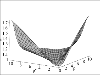
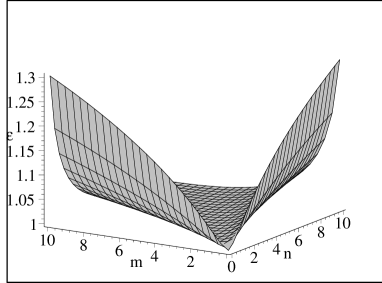
ab

Figure 1: The $\varepsilon$-factor for a free particle where momenta are given in $mc$ units (a) and for a relativistic rotator where the ratio of the Compton wavelength to the oscillator length is $\lambda=10$ (b).

Taking into account (ii), expression (30) for the even part of the Wigner function can be rewritten as follows:

$$W_{[\pm]}(p,q)=\pm\sum\limits_{n=0}^{\infty}W_{nn}(p,q)\left|C_{n;\pm}\right|^{2}+\sum\limits_{n\neq m}{\varepsilon(m,n)}W_{nm}(p,q)C_{m;}^{*}{}_{\pm}C_{n;}{}^{\pm}.$$ (68)

Therefore, the $\varepsilon$-factor affects the value of the interference terms only. Taking into account (iii), one can say, that it results in an effective increase in coherence between eigenstates of the Hamiltonian. Hence, information on the relative phase between $C_{n;\pm}$ becomes more evident; moreover, the value of this phase does not change.

It is worth noting, that this information can be lost. This is possible in the case where the particle interacts with an environment (or has interacted with it in the past) in such a way that they are in entangled state

$$\left|\Psi\right\rangle=\sum_{n=0}^{\infty}C_{n}\left|n\right\rangle\otimes\left|a(n)\right\rangle,$$ (69)

where $\left|n\right\rangle$ are the particle eigenstates and $\left|a(n)\right\rangle$ are macroscopically distinguishable states (generally not orthogonal) of an environment, which includes many degrees of freedom. In this and other equations, we do not write explicitly the symbols $\pm$.

The problem of decoherence is one of the most important in quantum information and quantum technologies (see, for example, [23] and references therein). Also, this problem has a fundamental meaning because it plays a crucial role in understanding the quantum measurement processes. We consider briefly this problem to clarify the possibility of using the nontrivial charge structure of the position (momentum) operator for suppressing the decoherence.

The density operator of the particle, considered as an open system, is the operator obtained after averaging of the pure state $\left|\Psi\right\rangle\left\langle\Psi\right|$ over the degrees of freedom of the environment

$$\hat{\rho}=\sum_{n,m=0}^{\infty}\left|n\right\rangle C_{m}^{*}C_{n}a(m,n)\left\langle m\right|,$$ (70)

where

$$a(m,n)=\left\langle a(m)|a(n)\right\rangle.$$ (71)

The Wigner function of this state in the nonlocal (nonrelativistic) theory can be written in the following form:

$$W(p,q)=\sum_{n,m=0}^{\infty}{a(m,n)}W_{nm}(p,q)C_{m}^{*}C_{n}.$$ (72)

This expression is very similar to (30) for the Wigner function for charge-invariant observables in the standard theory; $a(m,n)$ plays a role of the $\varepsilon$-factor here. From (71) the following properties of $a(m,n)$ follow:

1. Hermiticity, $a^{*}(n,m)=a(m,n)$;

2. Value of diagonal elements, $a(n,n)=1$;

3. Absolute value of nondiagonal elements, $\left|a(n,m)\right|<1$, if $n\neq m$.

Properties (i) and (ii) are identical to those of the $\varepsilon$-factor. However, as follows from (iii), the contribution of interference terms in the open system decreases. This is essence of the decoherence process. The $\varepsilon$-factor leads to the opposite result.

Consider the Wigner function for charge-invariant observables that represents the state of open system (70)

$$W_{[\pm]}(p,q)=\sum_{n,m=0}^{\infty}{a(m,n)\varepsilon(m,n)}W_{nm}(p,q)C_{m;}^{*}{}_{\pm}C_{n;}{}^{\pm}.$$ (73)

Due to the $\varepsilon$-factor, a contribution of interference terms increases here. Therefore, the nontrivial charge structure of the position (momentum) operators results in an effective increase in coherence between eigenstates of the Hamiltonian.

In figure 2 we present a plot of the Wigner function for the state of a relativistic rotator (see Appendix), which is the superposition of two eigenstates of the Hamiltonian, $\left|0\right\rangle$ and $\left|2\right\rangle$, for three different cases. Figure 2 a shows the Wigner function for the mixed state. Figure 2 b corresponds to the superposition in nonlocal theory (without decoherence). The contribution of interference terms appears in this example. Figure 2 c shows the Wigner function for charge-invariant observables in the standard theory. Interference terms play a more crucial role here.

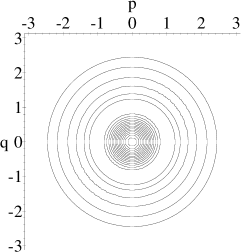
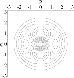
a b c

Figure 2: Contours of the Wigner function of a relativistic rotator for the mixed state $\hat{\rho}=1/2\Big{(}\left|0\right\rangle\left\langle 0\right|+\left|2\rangle\langle 2\right|\Big{)}$ (a) and for the superposition $\left|\psi\right\rangle=2^{-1/2}\Big{(}\left|0\right\rangle+\left|2\right\rangle\Big{)}$  (b) in nonlocal theory and in the standard theory with nontrivial charge structure of the position and momentum operators (c). The ratio of the Compton wavelength to the oscillator length is $\lambda=10$. Position and momentum are given in dimensionless units (see Appendix).

The Wigner function can be experimentally reconstructed in view of the quantum tomography method [24]. The problem regarding the consistent interpretation of the quadrature operator (or position and momentum operators) measurement arises here. Indeed, in the relativistic case, these operators, generally speaking, are not one-particle operators. The possibility of using the one-particle formalism has to be clarified in this case.

Our point of view is as follows. The consistent development of the relativistic quantum theory is possible within the framework of the second quantization method only. However, under conditions where the particle-pair creation does not take place, one can consider the one-particle sector of the theory. On the other hand, when one measures the quadrature (position, momentum) operator, the one-particle state is destroyed. From the viewpoint of measurement theory, the resulting state would be an eigenstate of the operator measured. However, This not possible because in this case one gets a state that is a superposition of states with different charge signs. One can suppose that this superposition is instantly destroyed. As a result, after a measurement we have a multi-particle state with pairs created from vacuum.

These assumptions explain why we call the increase in coherence in (73) the effective one. In fact, the coherence does not really increase (expression (70) does not contain the $\varepsilon$-factor). The peculiarities of the process of multi-particle operator measurement lead to such an effect.

There is the viewpoint that strongly localized states (with dispersion less than the Compton wavelength) in relativistic quantum mechanics do not exist. Indeed, for spin-0 particles, it leads to the appearance of states with negative dispersions [1]. However, in addition to the position dispersion, in real physical systems there exists an extra parameter (the characteristic length). For a relativistic rotator, it is the oscillator length (see Appendix), for a free particle it is $\hbar/\Delta p$, where $\Delta p$ is the momentum dispersion.

Generally speaking, there exists one more physical reason for the lower bound of the localization. This reason itself is related to the definition of the relativistic position operator, and follows from the inequality $\Delta v<c$; an analysis of this problem is given in [25]. It turned out, that it is possible to consider arbitrary localized states for particles with the energy $E\gg mc^{2}$.

In figure 3 we plot the Wigner function of a free particle for the state with the Gaussian distribution in the momentum space. The characteristic length of this state is 8 times less than the Compton wavelength. From this figure, one can see that the particle is localized in the $\lambda_{c}/8$ domain (of the order of the characteristic length). The vacuum processes lead to the appearance of specific perturbations, which gives a negative contribution into dispersion.

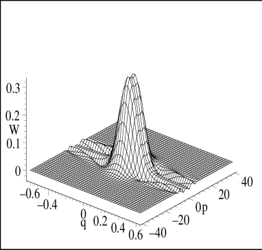
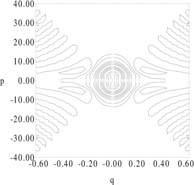
a b

Figure 3: The Wigner function (a) and its contours (b) for the Gaussin state of a free particle. The ratio of the Compton wavelength to the characteristic wave packet width is $\lambda=8$. Position is given in $\lambda_{c}=\hbar/mc$ units and momentum, in $mc$ units.

Another example is the eigenstate of a relativistic rotator. It can have an arbitrary small dispersion without any perturbation. This fact can be explained by Property 5 of the previous Section.

An additional difficulty in the experimental observation of these peculiarities is in the fact that they can appear in nonstationary process only. It is well known that interference terms oscillate with frequency

$$\omega_{mn}=\frac{E(m)-E(n)}{\hbar}.$$ (74)

The $\varepsilon$-factor is important in the case where the difference between energy levels is close to $mc^{2}$. Hence, to verify these peculiarities, one needs to control time intervals smaller than the Compton time

$$t_{c}=\frac{\hbar}{mc^{2}}.$$ (75)

For $\pi^{\pm}$ mesons, this time equals $4.7\cdot 10^{-24}$ s, for electrons, $1.3\cdot 10^{-21}$ s.

Similar peculiarities can appear in other systems with the band structure of energy spectrum. This can take place, for example, in semiconductors, where the analog of the Compton time is close to $10^{-15}$ s. The nontrivial charge structure of the position (momentum) operator, in this language, means that an eigenfunction of this operator is a superposition of the states of the conduction and valence bands. Measuring such an observable for conduction electrons results in a displacement of the electrons from the valence band to the conduction band and the appearance of electron–hole pairs.

7 Conclusions

In this work, we have considered some mathematical peculiarities of the phase space representation for spin-0 particles and their physical consequences. We have restricted ourselves by such a class of observables, whose matrix-valued Weyl symbols are proportional to the identity matrix. We call them charge-invariant observables. In fact, any combination of the position and momentum belongs to this class. However, such observables as energy and current are not charge-invariant ones due to the nontrivial dependence on the charge variable.

The time evolution in the standard theory is the same as in nonlocal theory, i.e., it does not depend on the nontrivial charge structure of position and momentum operators. However, in both cases the time evolution differs of the evolution of classical systems. The reason consists not only in the definition of the Moyal bracket and star-product. The classical Hamilton function does not coincide with symbol that plays the role of the Hamiltonian in the evolution equations. In the quantum case, the square root is determined by means of the star-product, and relativistic effects result both in a large value of the nonrelativistic Hamilton function (large momentum for the free particle case) and small characteristic length of the system.

The nontrivial charge structure of the position (momentum) operators leads to the peculiarities of the constraint on the Wigner function. However, they can appear in nonstationary processes only, including those that are described in nonequilibrium statistical physics. This can be explained by the peculiarities of the relativistic position (momentum) measurement. The initial one-particle state is destroyed in these processes. As a result, one obtains a multi-particle state. This leads to the appearance of additional multipliers for the interference terms between eigenstates of the Hamiltonian in the distribution function. These terms are responsible for the nonstationary processes.

It is very important that these multipliers ($\varepsilon$-factor) exceed unity. This means an effective increase in coherence in such systems (or, to be more precise, in such kinds of measurements). To verify this in the experiment, one needs to control time intervals close to the Compton time. However, such peculiarities can appear in other systems with the band structure of the energy spectrum. For example, one can use semiconductors where the analog of the Compton time is close to $10^{-15}$ s. We hope that such kinds of experiments are possible using modern devices.

Appendix. Relativistic rotator

Consider a particle in a constant homogeneous magnetic field and choose the vector potential in the form

$$\vec{A}=\frac{1}{2}\left[\vec{B}\times\vec{r}\right],$$ (76)

where $\vec{B}$ has only $z$ component

$$\vec{B}=\left(\begin{array}[]{c}0\\ 0\\ B\end{array}\right)$$ (77)

In this case, the Hamiltonian (3) can be written as follows [26]:

$$\hat{H}=\left(\tau_{3}+i\tau_{2}\right)\left(\frac{\hat{p}_{z}^{2}}{2m}+\frac{\hbar\omega_{c}}{2}\left(\hat{\pi}^{2}+\hat{\xi}^{2}\right)\right)+\tau_{3}mc^{2},$$ (78)

where $\omega_{c}=eB/m$ is the cyclotron frequency and $\hat{\pi}$ and $\hat{\xi}$ are dimensionless linear combinations of momentum and position. Their physical meaning consists in describing the particle position in a reference frame connected with the center of cyclotron motion.

In our consideration, we neglect the translation motion along the $z$ axis and consider the Hamiltonian of a relativistic rotator

$$\hat{H}=\frac{\hbar\omega_{c}}{2}\left(\tau_{3}+i\tau_{2}\right)\left(\hat{p}^{2}+\hat{q}^{2}\right)+\tau_{3}mc^{2}.$$ (79)

In the nonlocal theory representation, this Hamiltonian has a simple form

$$\hat{H}^{nl}=\tau_{3}mc^{2}\sqrt{1+\lambda^{2}\left(\hat{p}^{2}+\hat{q}^{2}\right)},$$ (80)

where $\lambda^{2}=\hbar\omega_{c}/mc^{2}$. In other words, if one considers the characteristic oscillator length $\sigma^{2}=\hbar/m\omega_{c}$, $\lambda$ is the ratio of the Compton wavelength and the characteristic oscillator length.

The energy spectrum for this problem, in agreement with (6), is expressed through the harmonic oscillator spectrum and can be written in the form

$$E(n)=mc^{2}\sqrt{1+2\lambda^{2}\left(n+\frac{1}{2}\right)}.$$ (81)

The matrix of the Hermitian generalization of the Wigner function for the relativistic rotator coincides with that used for the usual harmonic oscillator and is written in the following form [17]:

$$W_{nm} (p,q)=\frac{1}{\pi}\exp\left(-q^{2}-p^{2}\right)$$ (84)

$$\times \left\{\begin{array}[]{ll}\left(\sqrt{2}\left(q-ip\right)\right)^{n-m}(-1)^{m}\sqrt{\frac{m!}{n!}}L^{n-m}_{m}\left(2\left(p^{2}+q^{2}\right)\right)&\textrm{if $n\geq m$}\\ \left(\sqrt{2}\left(q+ip\right)\right)^{m-n}(-1)^{n}\sqrt{\frac{n!}{m!}}L^{m-n}_{n}\left(2\left(p^{2}+q^{2}\right)\right)&\textrm{if $n\leq m$}\end{array}\right.,$$

where $L^{k}_{l}(x)$ is the generalized Laguerre polynomial. For diagonal elements, it reads

$$W_{nn}(p,q)=\frac{1}{\pi}\exp\left(-q^{2}-p^{2}\right)(-1)^{n}L_{n}\left(2\left(p^{2}+q^{2}\right)\right).$$ (85)

Let us calculate the Hamiltonian (given for this problem by (42)). To do this, we use the fact that the Weyl symbol of an arbitrary operator $\hat{A}$ can be expressed through the matrix elements as follows:

$$A(p,q)=(2\pi)^{d}\sum_{n,m=0}^{\infty}A_{nm}W_{mn}(p,q).$$ (86)

In our case, this expression can be written in the form

$$E (p,q)=2\pi\sum_{n=0}^{\infty}E(n)W_{nn}(p,q)$$ (87)

$$= 2mc^{2}e^{-q^{2}-p^{2}}\sum_{n=0}^{\infty}\sqrt{1+2\lambda^{2}\left(n+\frac{1}{2}\right)}(-1)^{n}L_{n}\left(2\left(p^{2}+q^{2}\right)\right).$$

Consider the function

$$F(x,z)=\sum_{n=0}^{\infty}\sqrt{1+2\lambda^{2}\left(n+\frac{1}{2}\right)}L_{n}\left(x\right)z^{n}.$$ (88)

Using the fact that

$$n^{k}z^{n}=(z\partial_{z})^{k}z^{n},$$ (89)

in view of the identity for generating function for the Laguerre polynomials [27]

$$\sum_{n=0}^{\infty}L_{n}(x)z^{n}=\left(1-z\right)^{-1}\exp\left(\frac{zx}{z-1}\right)$$ (90)

one can write the function (88) in the following form:

$$F(x,z)=\sqrt{1+2\lambda^{2}\left(z\partial_{z}+\frac{1}{2}\right)}\left(1-z\right)^{-1}\exp\left(\frac{zx}{z-1}\right).$$ (91)

The Hamiltonian (87) in our representation can be written as follows:

$$E(p,q)=2mc^{2}\exp\left(-q^{2}-p^{2}\right)F\left(2\left(q^{2}+p^{2}\right),-1\right).$$ (92)

The term under the square root in (91) can be expanded in a power series and one can obtain the Hamiltonian with relativistic corrections; we will write it here up to the third-order terms

$$E(p,q)=mc^{2}+ \hbar\omega_{c}\left\{\frac{\lambda^{2}}{8}+\frac{1}{2}\left(p^{2}+q^{2}\right)\left(1-\frac{5\lambda^{4}}{8}\right)\right.$$ (93)

$$\left.-\frac{\lambda^{2}}{8}\left(p^{2}+q^{2}\right)^{2}+\frac{\lambda^{4}}{16}\left(p^{2}+q^{2}\right)^{3}+\ldots\right\}.$$

This expression differs from a similar expansion for the classical Hamilton function. Both the usual classical expression $\left(p^{2}+q^{2}\right)$ and $\lambda^{2}$ are independent relativistic parameters of the expansion.

References

- [1] Lev B I, Semenov A A and Usenko C V 2001 J. Phys. A 34 4323
- [2] Feshbach H and Villars F 1958 Rev. Mod. Phys. 30 24
-
[3]
Gavrilov S P and Gitman D M 2000 Int. J. Mod.
Phys A 15 4499
Gavrilov S P and Gitman D M 2000 Class. Quant. Grav. 17 L133
Gavrilov S P and Gitman D M 2001 Class. Quant. Grav. 18 2989 - [4] Newton T D and Wigner E P 1949 Rev. Mod. Phys. 21 400
- [5] Foldy L L and Wouthuysen S A 1950 Phys. Rev. 78 29
- [6] Silagadze Z K 1993 The Newton–Wigner position operator and the domain of validity of one-particle relativistic theory Preprint SLAC-PUB-5754 Rev
- [7] de Groot S R, van Leeuwen W A and van Weert Ch G 1980 Relativistic Kinetic Theory. Principles and Applications (Amsterdam: North-Holland)
- [8] Rukhadze A A and Silin V P 1960 Zh. Éksp. Teor. Fiz. 38 645
- [9] de Groot S R and Suttorp L G 1972 Fundations of Electrodynamics (Amsterdam: North-Holland)
-
[10]
Kim Y S and Wigner E P 1988 Phys. Rev. A 38
1159
Kim Y S and Wigner E P 1989 Phys. Rev. A 39 2829 - [11] Kim Chang-Ho and Kim Y S 1991 J. Math. Phys. 32 1998
-
[12]
Tomonaga S 1946 Prog. Theor. Phys. 1 27
Schwinger J 1948 Phys. Rev. 74 1439 -
[13]
Suarez A and Scarani V 1997 Phys. Lett. A 232
9
Zbinden H, Brendel J, Tittel W and Gisin N 2001 J. Phys. A 34 7103
Zbinden H, Brendel J, Gisin N and Tittel W 2001 Phys. Rev. A 63 02211
Stefanov A, Zbinden H and Gisin N 2001 Quantum corelations versus Multysimultaneity: an experiment test Preprint LANL quant-ph/0110117
Hacyan S. 2001 Phys. Lett. A 288 59 - [14] Bracken A J and Melloy G F 1999 J. Phys. A 32 6127
- [15] Lev B I, Semenov A A and Usenko C V 1997 Phys. Lett. A 230 261
-
[16]
Briegel H-J, Englert B-G, Michaelis M and Süssmann
G 1991 Z. Naturforsch. 46a 925
Briegel H-J, Englert B-G and Süssmann G 1991 Z. Naturforsch. 46a 933 - [17] Bartlett M S and Moyal J E 1949 Proc. Camb. Phil. Soc. 45 545
- [18] Curtright T, Uematsu T and Zachos C 2001 J. Math. Phys. 42 2396
- [19] Fairlie D 1964 Proc. Camb. Phil. Soc. 60 581
-
[20]
Wigner E P 1952 Z. Phys. 133 101
Wick G C, Wightman A S and Wigner E P 1952 Phys. Rev. 88 101 - [21] Grib A A, Mamaev S G and Mostepanenko V M 1988 Vacuum Quantum Effects in Strong Fields (Moscow: Energoatomizdat) (in Russian)
- [22] Tatarskii V I 1983 Sov. Phys.–Usp. 26 311
-
[23]
Joos E and Zeh H D 1985 Z. Phys. B 59 223
Joos E 1984 Phys. Rev. D 29 1626
Zurek W H 1981 Phys. Rev. D 24 1516
Zurek W H 1982 Phys. Rev. D 26 1862
Zurek W H 2001 Nature 412 712
Stodolsky L 1982 Phys. Lett. B 116 464
Menskii M B 2000 Phys.–Usp. 43 585
Kilin S Ya 1999 Phys.–Usp. 42 435 -
[24]
D’Ariano G M, Mancini S, Man’ko V I and Tombesi P
1996 Quant. Semiclass. Opt. 8 1017
Mancini S, Man’ko V and Tombesi P 1997 J. Mod. Opt. 44 2281 - [25] Dodonov V V and Mizrahi S S 1993 Phys. Lett. A 117 394
- [26] Johnson M H and Lippmann B A 1949 Phys. Rev. 76 828
- [27] Bateman H and Erdélyi A 1953 Higher Transcendental Functions (New York: McGraw-Hill)