Atom Lasers, Coherent States, and Coherence:
II. Maximally Robust Ensembles of Pure States

Abstract

As discussed in the preceding paper [Wiseman and Vaccaro, quant-ph/9906125], the stationary state of an optical or atom laser far above threshold is a mixture of coherent field states with random phase, or, equivalently, a Poissonian mixture of number states. We are interested in which, if either, of these descriptions of $\rho_{\rm ss}$ as a stationary ensemble of pure states, is more natural. In the preceding paper we concentrated upon the question of whether descriptions such as these are physically realizable (PR). In this paper we investigate another relevant aspect of these ensembles, their robustness. A robust ensemble is one for which the pure states that comprise it survive relatively unchanged for a long time under the system evolution. We determine numerically the most robust ensembles as a function of the parameters in the laser model: the self-energy $\chi$ of the bosons in the laser mode, and the excess phase noise $\nu$. We find that these most robust ensembles are PR ensembles, or similar to PR ensembles, for all values of these parameters. In the ideal laser limit ($\nu=\chi=0$), the most robust states are coherent states. As the phase noise or phase dispersion is increased through $\nu$ or the self-interaction of the bosons $\chi$, respectively, the most robust states become more and more amplitude-squeezed. We find scaling laws for these states, and give analytical derivations for them. As the phase diffusion or dispersion becomes so large that the laser output is no longer quantum coherent, the most robust states become so squeezed that they cease to have a well-defined coherent amplitude. That is, the quantum coherence of the laser output is manifest in the most robust PR ensemble being an ensemble of states with a well-defined coherent amplitude. This lends support to our approach of regarding robust PR ensembles as the most natural description of the state of the laser mode. It also has interesting implications for atom lasers in particular, for which phase dispersion due to self-interactions is expected to be large.

I Introduction

A laser is a device that produces a coherent beam of bosons. The meaning of the word ‘coherent’ in this context is discussed at length in a paper by one of us [1]. In particular, a coherent output does not mean that the output, or the laser mode itself, is in a coherent state. Rather, as has long been recognized [2], the stationary state matrix for the laser mode is a mixture of number states. In the far-above threshold limit, this mixture is Poissonian with mean $\mu$:

$$\rho_{\rm ss}=\sum_{n=0}^{\infty}e^{-\mu}\frac{\mu^{n}}{n!}\left|{n}\right\rangle\left\langle{n}\right|.$$ (1)

This state matrix can also be represented as a mixture of coherent states:

$$\rho_{\rm ss}=\int\frac{d\phi}{2\pi}\left|{|\alpha|e^{i\phi}}\right\rangle\left\langle{|\alpha|e^{i\phi}}\right|,$$ (2)

where $|\alpha|^{2}=\mu$.

On the basis of this second representation, one might claim that the laser really is in a coherent state $\left|{|\alpha|e^{i\phi}}\right\rangle$, but that one cannot know a priori what the phase $\phi$ is. In the preceding paper [3] we have investigated whether this claim is true. If it were true then there should be some way of finding out which coherent state the laser is in without affecting its dynamics. We found that if there is any self-energy in the laser mode (such as a $\chi^{(3)}$ nonlinearity for an optical laser, or $s$-wave scattering for an atom laser), then it is in fact not possible to physically realize the coherent state ensemble in Eq. (2). By contrast, it is always possible to physically realize the number state ensemble in Eq. (1).

For an ideal laser (with no $\chi^{(3)}$-like nonlinearity), the unknown coherent state description and the unknown number state description are both physically realizable (PR). Given that they are mathematically equivalent, why is the former description ubiquitous and the latter rare? The answer, as was pointed out some time ago by Gea-Banacloche [4], is differential survival times. An ideal laser prepared in a coherent state will remain close to that initial state for a time of order $\kappa^{-1}$, where $\kappa$ is the bare decay rate of the cavity. By contrast, a laser prepared in a number state will be likely to remain in that state only for a time of order $\kappa^{-1}/\mu$, where $\mu$ is the mean number as above.

This result, derived also in Ref. [5], was taken further by Gea-Banacloche in Ref. [6] using the early model for a laser with saturation due to Scully and Lamb [2]. Gea-Banacloche considered pure states with mean photon number equal to that of the laser at steady state, and calculated their purity at later times. He showed that the pure state that had the slowest initial rate of decay of purity was, in general, a slightly amplitude-squeezed state rather than a coherent state.

There seems little doubt, then, that it is most useful to consider an ideal laser to be in a coherent state (or nearly coherent state) of unknown phase. However it is an open question whether this is true of a non-ideal laser, that is, a laser with additional noise or dispersion of some form. Another open question is how this issue relates to the quantum coherence of the output of such a non-ideal device.

The particular laser system of interest here is the atom laser [1]. An important difference between an atom laser and an optical laser is that the interatomic interactions cannot be neglected. This gives rise to a $\chi^{(3)}$-like nonlinearity in the laser mode. As noted above, this affects the physical realizability of ensembles, and we also expect it to affect their robustness.

A robustness analysis for a Bose-Einstein condensate has been done by one of us with Barnett and Burnett [7]. This produced similar results to that of Gea-Banacloche [6], although it was based on the fidelity [8] which measures the overlap of the initial state with the state at a later time. However, the authors of Ref. [7] only calculated the initial rate of decay of the fidelity, and this is unaffected by any Hamiltonian terms. Hence the self energy played no role in this analysis. Moreover, the treatment, like that of Gea-Banacloche [6], considered only a single pure state to represent the state of the condensate. Thus it does not give, in general, a representation of the steady state on par with Eq. (1) or Eq. (2).

In this paper we give an analysis that treats the dynamics of an atom laser at all times and that incorporates an ensemble of pure states. It takes into account Hamiltonian terms and gives a robust representation of the steady state. We consider both the problem of finding the most robust ensemble, and the most robust physically realizable (PR) ensemble. Since ensembles are realized by unraveling the master equation [9, 3], finding the most robust PR ensemble is equivalent to finding the maximally robust unraveling, a concept introduced by us in Ref. [9].

A review of maximally robust unravelings, including a comparison with other approaches, is given in Sec. II. In Sec. III we present the equations for determining the maximally robust unraveling (MRU) for an atom laser model. We concentrate upon continuous Markovian unravelings, which give ensembles of Gaussian states, and also consider unconstrained Gaussian ensembles. In Sec. IV we present the numerical solutions for these equations, concentrating on the asymptotic behaviour in the limit of large nonlinearity $\chi$ and phase noise $\nu$. The concluding Sec. V is a discussion of our results and their relation to atom laser coherence, and some suggestions for future work.

II Maximally Robust Unravelings

A Comparison with Other Approaches

The idea of robustness has it origins in studies of decoherence and the classical limit [4, 5, 6, 7, 10, 11, 12, 13, 14, 15]. Decoherence is the process by which an open quantum system becomes entangled with its environment, thereby causing its state to become mixed. However, not all pure states decohere with equal rapidity. In particular, Zurek [10] defined the “preferred states” of open quantum systems as those states that remain relatively pure for a long time. This idea can be thought of as a “predictability sieve” [11]. That is, the preferred states are those for which the future dynamics are predictable, in the sense that there is some projective question (is the system in some particular state?) that is likely to give the result “yes”.

Our approach, as introduced in Ref. [9] and applied to resonance fluorescence by one of us and Brady [16], is to find the maximally robust unraveling. This approach shares some similarities with other approaches. It has, however, a suite of four distinctive characteristics which we enumerate below.

1 Ensembles of Pure States

First, we considered not a single pure state, but an ensemble of pure states. This is appropriate for situations where the open system comes to a mixed equilibrium state. The ensemble of pure states that we consider must be a representation of that equilibrium mixed state. That is, the system has a certain probability of being in one of those pure states, as in Eqs. (1) and (2). Recently, Diósi and Kiefer [14] have also considered ensembles of pure states in a similar context.

Without considering such an ensemble it is necessary to put some ad-hoc restriction on the pure states considered so that they have some relevance to the actual state the system is in at equilibrium. For example, as noted above, Gea-Banacloche [6] considered only pure states having the same mean photon number as the equilibrium state of the laser model under consideration.

2 Physical Realizability

Second, in Ref. [9] we placed a restriction on the ensembles of pure states that we consider: they must be physically realizable. By this we mean that it should be possible, without altering the evolution of the system, to know that its state at equilibrium is definitely one of the pure states in the ensemble, but which pure state cannot be predicted beforehand. Diósi and Kiefer [14] have considered a similar condition, although they do not make the connection with physical realizability and measurement. In this paper we also consider ensembles without the constraint of physical realizability, as it is of interest to see how active that constraint is.

We have considered in detail the issue of physical realizability of ensembles of pure states in the preceding paper [3]. Here we merely remind the reader of some key points and terminology. An ensemble for a system obeying a Markovian master equation is physically realized by monitoring the baths to which it is coupled. This leads to an unraveling [17] of the master equation into a stochastic equation for a pure state. In steady, state, the pure state will move ergodically within some (perhaps infinite) ensemble of pure states. This is how an unraveling defines an ensemble, with the weighting of each member being the proportion of time the system spends with that state.

3 Survival Probability

Third, in Ref. [9] we defined robustness in terms of the fidelity or survival probability of the pure states rather than their purity. That is, we consider how close the states remain to their original state under the master equation evolution, rather than just how close they remain to a pure state. This means that Hamiltonian evolution alone can affect the robustness of states (whereas it does not affect their purity, except in conjunction with the irreversible terms). It might be thought that this is an undesirable feature. However, as will be shown, using the survival probability gives results that accord with the usual concept of coherence in lasers. This contrasts with the results that are obtained using purity, which we also consider at the end of this paper (Sec. V C)

4 Survival Time

The final aspect of our work that differs from most previous approaches [6, 12, 13, 14] is that we quantify the robustness by the survival time. (This time was previously called the fidelity time in Ref [7]). It is the time taken for the survival probability to fall below some predefined threshold. This is as opposed to considering the rate of decay of the survival probability at the initial time. That rate is actually identical to half the initial rate of decay of the purity, and hence is independent of any Hamiltonian terms. It is only by considering the robustness over some finite time that the Hamiltonian terms will contribute.

B Unraveling the Master Equation

In this section, we briefly reiterate the discussion in Ref. [3] on how the master equation is unraveled to yield a pure state ensemble. The most general form of the Markovian master equation is [18]

$$\dot{\rho}=-i[H,\rho]+\sum_{k=1}^{K}{\cal D}[c_{k}]{\rho}\equiv{\cal L}\rho,$$ (3)

where for arbitrary operators $A$ and $B$,

$${\cal D}[A]B\equiv ABA^{\dagger}-\{A^{\dagger}A,B\}/2.$$ (4)

We assume this to have a unique stationary state $\rho_{\rm ss}$. It can be represented in terms of pure states as

$$\rho_{\rm ss}=\sum_{n}\wp_{n}P_{n},$$ (5)

where the $P_{n}$ are projection operators and the $\wp_{n}$ are positive weights summing to unity. The (possibly infinite) set of ordered pairs,

$$E=\{(P_{n},\wp_{n}):n=1,2,\ldots\},$$ (6)

we will call an ensemble $E$ of pure states. There are continuously infinitely many ensembles $E$ that represent $\rho_{\rm ss}$. Our aim is to find the ‘best’ or ‘most natural’ representation for $\rho_{\rm ss}$.

Our first requirement is that the ensemble be physically realizable. This is possible if the environment of the system is monitored, leading to a stochastic quantum trajectory for the system state. Assuming that the initial state of the system is pure, the quantum trajectory for its projector will be described by the stochastic master equation (SME)

$$d{P}=dt\left[{\cal L}+{\cal U}(t)\right]P.$$ (7)

Here the superoperator ${\cal U}$, which we will call an unraveling, does not affect the average evolution of the system, but preserves the idempotency of $P$. In the long-time limit the system will be in some pure state $P_{n}$, with some probability $\wp_{n}$ such that Eq. (5) is satisfied. Since the states and weights will depend on the unraveling ${\cal U}$, we denote the resultant stationary ensemble by

$$E^{\cal U}=\{(P_{n}^{\cal U},\wp_{n}^{\cal U}):n=1,2,\ldots\}.$$ (8)

For practical reasons explained in [3], we restrict our investigation of the (atom) laser to continuous Markovian unravelings (CMUs). As was shown in [3], under a linearization of the dynamics these lead to Gaussian pure states as the members of the ensembles $E^{\cal U}$. As mentioned above, we will also consider ensembles, in particular Gaussian ensembles, which are not constrained by the requirement of physical realizability. This is in order to see the importance of this requirement in constraining the most natural ensembles.

C Quantifying the Robustness

1 Survival Probability

Imagine that the system has been evolving under a particular unraveling ${\cal U}$ from an initial state at time $-\infty$ to the stationary ensemble at the present time $0$. It will then be in the state $P_{n}^{\cal U}$ with probability $\wp_{n}^{\cal U}$. If we now cease to monitor the system then the state will no longer remain pure, but rather will relax toward $\rho_{\rm ss}$ under the evolution of Eq. (3).

This relaxation to equilibrium will occur at different rates for different states. For example, some unravelings will tend to collapse the system at $t=0$ into a pure state that is very fragile, in that the system will not remain in that state for very long. In this case the ensemble would rapidly become a poor representation of the observer’s current knowledge about the system. Hence we can say that such an ensemble is a ‘bad’ or ‘unnatural’ representation of $\rho$. Conversely, an unraveling that produces robust states would remain an accurate description for a relatively long time. We expect such a ‘good’ or ‘natural’ ensemble to give more intuition about the dynamics of the system. The most robust ensemble we interpret as the ‘best’ or ‘most natural’ such ensemble.

In most of this paper we quantify the robustness of a particular state $P_{n}^{\cal U}$ by its survival probability $S_{n}^{\cal U}(t)$. This is the probability that the system would be found (by a hypothetical projective measurement) to be still in the state $P_{n}^{\cal U}$ at time $t$. It is given by [19]

$$S_{n}^{\cal U}(t)={\rm Tr}[P_{n}^{\cal U}e^{{\cal L}t}P_{n}^{\cal U}].$$ (9)

Since we are considering an ensemble $E^{\cal U}$ we must define the average survival probability

$$S^{\cal U}(t)=\sum_{n}\wp_{n}^{\cal U}S_{n}^{\cal U}(t).$$ (10)

In the limit $t\to\infty$ the ensemble-averaged survival probability will tend towards the stationary value

$$S^{\cal U}(\infty)={\rm Tr}[\rho_{\rm ss}^{2}].$$ (11)

This is independent of the unraveling ${\cal U}$ and is a measure of the mixedness of $\rho_{\rm ss}$.

2 Comparison with Purity

As noted in Sec. II A 3 above, it is more common in discussions of robustness to use purity rather than survival probability. The purity of a state at time $t$ can be quantified as

$$p^{\cal U}_{n}(t)={\rm Tr}[\left(e^{{\cal L}t}P_{n}^{\cal U}\right)^{2}].$$ (12)

The ensemble average of this quantity is also initially unity, and approaches ${\rm Tr}[\rho_{\rm ss}^{2}]$ as $t\to\infty$. Alternatively, the purity could be quantified as the maximum overlap of any pure state $\tilde{P}_{n}(t)$ with the evolved mixed state:

$$\tilde{p}^{\cal U}_{n}(t)={\rm max}_{\tilde{P}_{n}(t)}{\rm Tr}[\tilde{P}_{n}(t)\left(e^{{\cal L}t}P_{n}^{\cal U}\right)].$$ (13)

For Gaussian states (see Sec. III) these quantities are simply related by $\tilde{p}^{\cal U}_{n}(t)=2/[1+1/p^{\cal U}_{n}(t)]$.

The survival probability has a number of advantages over purity. First, we motivated our robustness criterion from the desire for $E^{\cal U}$ to remain a good description of the system once the unraveling ceases. That is, we wish to be able to usefully regard the members of the ensemble $E^{\cal U}$ as the states the system is “really” in at steady state. This is better quantified by the survival probability because the purity effectively takes into account only how close the state $e^{{\cal L}t}P_{n}$ remains to some pure state $\tilde{P}_{n}(t)$ [introduced in Eq. (13)], not how close it remains to the original state $P_{n}$. An ensemble constructed by considering the purity would thus, in general, only remain a good description of the system by including the deterministic (but not necessarily unitary) evolution of its members from $P_{n}$ to $\tilde{P}_{n}(t)$ after the unraveling ceases. This time evolution would negate the idea that the ensemble of states $P_{n}$ is the best representation of the system at steady state.

Another reason for preferring the survival probability comes from imagining that the unraveling ${\cal U}$ continues after $t=0$. In that case one can calculate a conditional survival probability, being the overlap of the pure conditional state with the pure initial state. The ensemble average of this conditional survival probability is simply the survival probability $S_{n}^{\cal U}(t)$ defined in Eq. (9) above. Thus the concept of survival probability still applies even for the conditional evolution. By contrast, the conditional purity of the unraveled state would always be unity, and consequently has no relation to the unconditional purity defined in Eq. (12). The latter thus has no simple interpretation for the unraveled evolution.

The final reason for preferring survival probability, already noted in Sec. II A 3, is that it yields results for the atom laser that have a clear and simple physical interpretation in terms of the coherence of the laser output. We will show that this is so in the Discussion section.

One limit in which quite different results are to be expected from using purity rather than survival probability is that in which the Hamiltonian part of the dynamics dominates. As will be shown, this limit is highly relevant for the atom laser.

Formally, we split the Liouvillian superoperator ${\cal L}$ as

$${\cal L}={\cal L}_{\rm irr}+\chi{\cal L}_{\rm rev},$$ (14)

where $\chi$ is a large parameter and

$${\cal L}_{\rm irr}\rho = \sum_{k=1}^{K}{\cal D}[c_{k}]\rho.$$ (15)

$${\cal L}_{\rm rev}\rho = -i[H,\rho].$$ (16)

The reversibility of ${\cal L}_{\rm rev}$ implies that

$${\rm Tr}[A{\cal L}_{\rm rev}B]=-{\rm Tr}[B{\cal L}_{\rm rev}A]$$ (17)

and so ${\rm Tr}[A{\cal L}_{\rm rev}A]=0$, for arbitrary operators $A$ and $B$.

To first order in time, both the survival probability and the purity depend only upon the irreversible term:

$$S(t) = 1+t{\rm Tr}[P{\cal L}_{\rm irr}P],$$ (18)

$$p(t) = 1+2t{\rm Tr}[P{\cal L}_{\rm irr}P].$$ (19)

For longer times, both expressions will (in general) be dominated in the large-$\chi$ regime by the reversible term, but in different ways:

$$S(t) \simeq 1+\chi^{2}(t^{2}/2){\rm Tr}[P{\cal L}_{\rm rev}^{2}P],$$ (20)

$$p(t) \simeq 1+\chi t^{2}{\rm Tr}[P({\cal L}_{\rm irr}{\cal L}_{\rm rev}-{\cal L}_{\rm rev}{\cal L}_{\rm irr})P].$$ (21)

The Hamiltonian term directly affects the survival probability, but it affects the purity only in combination with the irreversible term.

3 Survival Time

The above analysis shows that the difference between purity and survival probability only shows up at finite times. Thus the best way to characterize robustness is to look not at the initial rate of decay of the survival probability, but at the time it takes to fall below some threshold value $\Lambda$ satisfying

$$1>\Lambda>{\rm Tr}[\rho_{\rm ss}^{2}].$$ (22)

The ensemble survival time for a particular unraveling would then be defined as

$$\tau^{\cal U}={\rm min}\{t\,:\,S^{\cal U}(t)=\Lambda\}.$$ (23)

Note that this time is the first time for which $S^{\cal U}(t)=\Lambda$. The survival probability is not necessarily monotonically decreasing and in some simple examples there will be many solutions to the equation $S^{\cal U}(t)=\Lambda$ [16].

A natural choice of $\Lambda$, suggested in Ref. [9], is the maximum eigenvalue of $\rho_{\rm ss}$:

$$\Lambda = \lim_{n\to\infty}\left({\rm Tr}[\rho_{\rm ss}^{n}]\right)^{1/n}$$ (24)

$$= {\rm max}\{\lambda_{j}\in I\!\!R\,:\,\rho_{\rm ss}Q_{j}=\lambda_{j}Q_{j},Q_{j}=Q_{j}^{2}\}.$$ (25)

This can be shown to satisfy $\Lambda>{\rm Tr}[\rho_{\rm ss}^{2}]$ as follows. Let the eigenvalues of $\rho_{\rm ss}$ be ordered such that $\Lambda=\lambda_{1}\geq\lambda_{2}\geq\lambda_{3}\ldots$. Then

$${\rm Tr}[\rho_{\rm ss}^{2}] = \Lambda^{2}+\sum_{j=2}\lambda_{j}^{2}$$ (26)

$$< \Lambda^{2}+\sum_{j=2}\Lambda\lambda_{j}$$ (27)

$$= \Lambda^{2}+\Lambda(1-\Lambda)=\Lambda.$$ (28)

Here the strict inequality holds unless all eigenvalues of $\rho_{\rm ss}$ are equal.

In the absence of any monitoring of the bath, the projector $Q_{1}$ would be one’s best guess for what pure state the system is in at steady state. The chance of this guess being correct is simply $\Lambda$, which is obviously independent of time $t$. Using this $\Lambda$, the survival time $\tau^{\cal U}$ could thus be interpreted as the time at which the initial state $P^{\cal U}_{n}$ ceases (on average) to be any better than $Q_{1}$ as an estimate of which pure state is occupied. In other words, the ensemble $E^{\cal U}$ is obsolete at time $\tau^{\cal U}$.

In this paper we do not use this choice for $\Lambda$, for reasons to be explained later. This brings a certain degree of arbitrariness into the analysis. However, as we show, the most important and interesting results we obtain are independent of the choice of $\Lambda$.

Having chosen a particular value for $\Lambda$, the survival time $\tau^{\cal U}$ quantifies the robustness of an unraveling ${\cal U}$. Let the set of all unravelings be denoted $J$. Then the subset of maximally robust unravelings $J_{M}$ is

$$J_{M}=\{{\cal R}\in J:\tau^{\cal R}\geq\tau^{\cal U}\;\forall\,{\cal U}\in J\}.$$ (29)

As noted above, in practice it may be necessary to restrict the analysis to continuous Markovian unravelings $D$, and the corresponding subset $D_{M}$. Even if $J_{M}$ has many elements ${\cal R}_{1},{\cal R}_{2},\cdots$, these different unravelings may give the same ensemble $E^{\cal R}=E^{{\cal R}_{1}}=E^{{\cal R}_{2}}=\cdots$. In this case $E^{\cal R}$ is the most natural ensemble representation of the stationary solution of the given master equation. When we consider ensembles that are not constrained by the condition of physical realizability, we will denote the most robust of these by $E^{\rm R}$. That is, we reserve the calligraphic ${\cal R}$ to denote a robust unraveling.

III MRUs for The (Atom) Laser

A The Master Equation

The master equation we use for the (atom) laser is the same as that in the preceding paper [3]. In the interaction picture, and measuring time in units of the output decay rate, it is

$$\dot{\rho} = \left(\mu{\cal D}[a^{\dagger}]{\cal A}[a^{\dagger}]^{-1}+{\cal D}[a]+N{\cal D}[a^{\dagger}a]\right)\rho$$ (31)

$$-\,iC[(a^{\dagger}a)^{2},\rho].$$

The parameters $N$ and $C$ represent excess phase noise and self-interaction energy respectively. This has the stationary solution expressed in Eqs. (1) and (2), with mean boson number $\mu$.

To make progress on this equation we linearized it around a mean field by making the replacement

$$a=\sqrt{\mu}+(x+iy)/2,$$ (32)

with $x$ and $y$ Hermitian. The linearized master equation has a Gaussian solution with moments

$$\mu_{mn}=\left\langle{(x^{m}y^{mn})_{\rm sym}}\right\rangle$$ (33)

given by

$$\mu_{10}(t) = \mu_{10}(0)w,$$ (34)

$$\mu_{01}(t) = \mu_{01}(0)-\chi\mu_{10}(0)(1-w),$$ (35)

$$\mu_{20}(t) = \mu_{20}(0)w^{2}+1-w^{2},$$ (36)

$$\mu_{11}(t) = \mu_{11}(0)w-\chi\left\{1+w[\mu_{20}(0)-2]\right.$$ (38)

$$\left.\phantom{\mu_{11}(0)w-\chi\left\{\right.}+\,w^{2}[1-\mu_{20}(0)]\right\},$$

$$\mu_{02}(t) = \mu_{02}(0)+(2+\nu)t-2\chi\mu_{11}(0)(1-w)$$ (41)

$$+\,2\chi^{2}\left\{t+[\mu_{20}(0)-2](1-w)\right.$$

$$\left.\phantom{2\chi^{2}\left\{\right.t}+\,[1-\mu_{20}(0)](1-w^{2})/2\right\},$$

where $w\equiv e^{-t}$, $\chi=4\mu C$ and $\nu=4\mu N$. The long-time limit of this is a Wigner function

$$W_{\rm ss}(x,y)\propto\exp(-x^{2}/2)$$ (42)

with amplitude quadrature ($x$) variance of unity and phase quadrature ($y$) variance of infinity. This is what is expected as the linearized version of the stationary state of Eq. (1).

The conditions for the output of the laser to be coherent, in the sense of having an atom flux much greater than the linewidth (as conventionally defined) are simply stated in terms of the dimensionless self-energy $\chi$ and excess phase diffusions $\nu$ [3]

$$\chi \ll \mu^{3/2},$$ (43)

$$\nu \ll \mu^{2}.$$ (44)

B The Unraveled Master Equation

Under a continuous Markovian unraveling the long-time solutions for the linearized stochastic dynamics are still Gaussian [3]. In fact, the evolution of the second order moments $\mu_{20},\mu_{02},\mu_{11}$ is deterministic. This means that for a given unraveling ${\cal U}$ the stationary ensemble will consist of Gaussian pure states all having the same second order moments. They are distinguished only by their first order moments $\bar{x}=\mu_{10},\bar{y}=\mu_{01}$, which therefore take the role of the index $n$ in Eq. (8). The different ensembles themselves are indexed by another pair of numbers, $\mu_{11},\mu_{20}$, which play the role of ${\cal U}$ in Eq. (8). We do not need $\mu_{02}$ because the purity of the unraveled states implies that

$$\mu_{20}\mu_{02}-\mu_{11}^{2}=1.$$ (45)

However, it should be noted that the mapping from ${\cal U}$ to $\mu_{11},\mu_{20}$ is, in general, many-to-one.

The ensemble can thus be represented as

$$E^{\cal U}=\{(P^{\cal U}_{\bar{x},\bar{y}},\wp^{\cal U}_{\bar{x},\bar{y}}):{\bar{x},\bar{y}}\},$$ (46)

where the second order moments of the pure state $P^{\cal U}_{\bar{x},\bar{y}}$ are determined by the unraveling ${\cal U}$.

The weighting function is flat for $\bar{y}$ and for $\bar{x}$ is given by [3]

$$\wp^{\cal U}(\bar{x})=[2\pi(1-\mu_{20})]^{-1/2}\exp\left\{-\bar{x}^{2}/[2(1-\mu_{20})]\right\}.$$ (47)

It is convenient to use a new notation for the second order moments,

$$\alpha = \frac{\mu_{02}}{\mu_{20}\mu_{02}-\mu_{11}^{2}},$$ (48)

$$\beta = \frac{\mu_{11}}{\mu_{20}\mu_{02}-\mu_{11}^{2}},$$ (49)

$$\gamma = \frac{\mu_{20}}{\mu_{20}\mu_{02}-\mu_{11}^{2}}.$$ (50)

For pure states satisfying Eq. (45), we have (as in the preceding paper [3])

$$\alpha=\mu_{02}\;;\;\;\beta=\mu_{11}\;;\;\;\gamma=\mu_{20},$$ (51)

The different ensembles are now indexed by the pair $\beta,\gamma$. Not all pairs $\beta,\gamma$ correspond to physically realizable ensembles. The method for determining which do correspond to PR ensembles is described in the preceding paper [3], and the constraints that apply are simply $\gamma>0$ and

$$(-2\chi\beta+2+\nu)(-2\gamma+2)-(\beta+\chi\gamma)^{2}\geq 0.$$ (52)

C Survival Probability

We are interested in the survival probability of the states $P^{\cal U}_{\bar{x},\bar{y}}$. It is convenient to consider the corresponding Wigner functions, $W^{\cal U}_{\bar{x},\bar{y}}(x,y)$. Obviously the survival probability is independent of $\bar{y}$ so we will drop this subscript, and set $\bar{y}=0$ for ease of calculation. For Gaussian states the Wigner function is a bivariate Gaussian distribution with the moments $\mu_{mn}$ defined above. The state with initial moments $\mu_{mn}(0)$ will evolve into a state with moments $\mu_{mn}(t)$ given by (34–41). We will denote the Wigner function for the former state $W_{\bar{x}}(x,y,0)$ and that for the latter $W_{\bar{x}}(x,y,t)$. The survival probability of the state $P_{\bar{x}}^{\cal U}$ is given by [20]

  

$$S_{\bar{x}}(t) \equiv {\rm Tr}[P_{\bar{x}}e^{{\cal L}t}P_{\bar{x}}]=4\pi\int dxdyW_{\bar{x}}(x,y,0)W_{\bar{x}}(x,y,t)$$ (53)

$$= 4\pi\int dxdy{\cal N}(0)\exp\left[\frac{\mu_{20}(0)\mu_{02}(0)}{\mu_{20}(0)\mu_{02}(0)-\mu_{11}(0)^{2}}\left(-\frac{(x-\bar{x})^{2}}{2\mu_{20}(0)}+\frac{\mu_{11}(0)(x-\bar{x})y}{\mu_{20}(0)\mu_{02}(0)}-\frac{y^{2}}{2\mu_{02}(0)}\right)\right]$$ (55)

$$\times\;{\cal N}(t)\exp\left[\frac{\mu_{20}(t)\mu_{02}(t)}{\mu_{20}(t)\mu_{02}(t)-\mu_{11}(t)^{2}}\left(-\frac{(x-\bar{x}w)^{2}}{2\mu_{20}(t)}+\frac{\mu_{11}(t)(x-\bar{x}w)(y+\chi\bar{x}(1-w))}{\mu_{20}(t)\mu_{02}(t)}-\frac{(y+\chi\bar{x}(1-w))^{2}}{2\mu_{02}(t)}\right)\right],$$

where

$${\cal N}=\left(2\pi\sqrt{\mu_{20}\mu_{02}-\mu_{11}^{2}}\right)^{-1}.$$ (56)

This survival probability should be averaged over all $\bar{x}$, weighted by the distribution (47) to get

$$S^{\cal U}(t)=\int d\bar{x}S_{\bar{x}}(t)\wp^{\cal U}(\bar{x}).$$ (57)

Thus $S(t)$ is given by a triple Gaussian integral that evaluates to the following:

$$S^{\cal U}(t)=2\sqrt{\frac{(\alpha_{t}\gamma_{t}-\beta_{t}^{2})/[1+(1-\gamma_{0})R_{t}]}{(\alpha_{0}+\alpha_{t})(\gamma_{0}+\gamma_{t})-(\beta_{0}+\beta_{t})^{2}}}$$ (58)

where

$$R_{t} = \alpha_{0}+\alpha_{t}w^{2}+2\beta_{t}\chi wz+\gamma_{t}\chi^{2}z^{2}-\frac{(\alpha_{0}+\alpha_{t}w+\beta_{t}\chi z)^{2}}{\alpha_{0}+\alpha_{t}}$$ (60)

$$\ \ \-\frac{\big{[}(\beta_{0}+\beta_{t})(\alpha_{0}+\alpha_{t}w+\beta_{t}\chi z)-(\alpha_{0}+\alpha_{t})(\beta_{0}+\beta_{t}w+\gamma_{t}\chi z)\big{]}^{2}}{(\alpha_{0}+\alpha_{t})[(\alpha_{0}+\alpha_{t})(\gamma_{0}+\gamma_{t})-(\beta_{0}+\beta_{t})^{2}]},$$

  

where $z\equiv 1-w$ and $\alpha,\beta,\gamma$ are as in Eqs. (48)–(50), and $\mu_{mn}$ are as in Eqs. (34)–(41). Note that at $t=0$ the state is pure, so that $\alpha_{0}=\mu_{02},\beta_{0}=\mu_{11},\gamma_{0}=\mu_{20}$ as previously. The survival probability $S^{\cal U}(t)$ is thus a function of the initial state parameters $\gamma_{0}$ and $\beta_{0}$, and the dynamical parameters $\nu$ and $\chi$.

D The Survival Time

Following the general theory described in Sec. II C 3, we define the survival time $\tau^{\cal U}$ as the smallest (in this case it will be the only) solution to the equation

$$S^{\cal U}(\tau^{\cal U})=\Lambda,$$ (61)

where $\Lambda$ is a constant satisfying

$$1>\Lambda>{\rm Tr}[\rho_{\rm ss}^{2}].$$ (62)

From the solution (1) of the nonlinear dynamics, the lower bound on $\Lambda$ is, for $\mu\gg 1$,

$${\rm Tr}[\rho_{\rm ss}^{2}]=(4\pi\mu)^{-1/2}.$$ (63)

In the same limit, the largest eigenvalue for $\rho_{\rm ss}$ is

$$\lim_{n\to\infty}\sqrt[n]{{\rm Tr}[\rho_{\rm ss}^{n}]}=(2\pi\mu)^{-1/2}.$$ (64)

From these expressions it is evident that there would be a problem in choosing Eq. (64) for $\Lambda$: it is very close to the value for ${\rm Tr}[\rho_{\rm ss}^{2}]=(4\pi\mu)^{-1/2}$. This means that the survival time would be equal to the time by which the system has relaxed almost to the equilibrium mixed state. In particular, its phase would necessarily be poorly defined by this time, which means that the linearization of the dynamics that we have been using would not be valid.

If instead we start with the solution (42) of the linearized dynamics, we have an even worse situation:

$${\rm Tr}[\rho_{\rm ss}^{2}]=\lim_{n\to\infty}\sqrt[n]{{\rm Tr}[\rho_{\rm ss}^{n}]}=0.$$ (65)

In this case the survival time would always be infinite, which is not helpful.

Because of these problems, we have not chosen the largest eigenvalue of $\rho_{\rm ss}$ for $\Lambda$. Instead we have investigated the dependence of $\tau^{\cal R}$ on $\Lambda$ for various values, namely $\Lambda=0.5,0.2,0.1,0.05$. As will be shown, the most robust ensemble, (that with the largest survival time) is substantially independent of $\Lambda$. Unless otherwise stated we choose $\Lambda$ to be the midpoint of the two bounds in Eq. (62), namely

$$\Lambda=1/2.$$ (66)

E Unconstrained Gaussian Ensembles

Finding the most robust PR ensemble $E^{\cal R}$ consists of a searching for the maximum $\tau$ in the region of $\beta$-$\gamma$ space allowed by the PR constraint. To determine how important this constraint is in determining $E^{\cal R}$, we also search for the maximum $\tau$ in all of $\beta$-$\gamma$ space (subject only to $0<\gamma\leq 1$). The ensemble picked out by this search we will call the most robust unconstrained ensemble and denote $E^{\rm R}$. Although we call in unconstrained, it is in fact constrained to be of the same form as the ensembles resulting from a continuous Markovian unravelings. That is, it consists of Gaussian states with identical second-order moments distinguished only by their mean amplitude and phase.

IV Results

A Varying $\chi$ with $\nu=0$

First we present the results for no excess phase noise ($\nu=0$) to see the effect of varying the self-energy parameter $\chi$. Because our results are numerical, we present them mostly in a graphical form.

1 Evolution at $\chi=0$ and $\chi=50$

Fig. 1 shows the evolution of various initially pure Gaussian quantum states under the linearized evolution of Eqs. (34)–(41). We represent these states by the one-standard-deviation ellipses of the Wigner function. In each case we choose the initial mean location of the state in phase space to be $\bar{x}=\bar{y}=0$, and, for the last two cases, for $\bar{y}=0$, $\bar{x}=\pm\sqrt{3/2}$ as well.

The first case in Fig. 1(a) is for $\nu=0,\chi=0$, and an initial coherent state. The ellipses are plotted for $t=0,3,10$. The middle time is the ensemble-averaged survival time for an ensemble of coherent states; that is, the time at which the ensemble-averaged survival probability $S(t)$ drops to $1/2$. For the particular case of the coherent state there is no distinction between the ensemble-averaged survival probability and the survival probability of a single coherent state $S_{\bar{x}}(t)$. That is because the $x$-variance $\gamma$ of a coherent state is equal to unity, the ensemble-averaged $x$-variance, so that perforce $\bar{x}=0$. Note that the only dynamics in evidence here is phase diffusion, causing the $y$-variance of the state to increase. For $\chi=\nu=0$, the coherent state ensemble is in fact the most robust ensemble. This can be verified analytically. It is also physically realizable, as shown in the preceding paper [3].

The second case in Fig. 1(b) is again for an initial coherent state but with $\nu=0,\chi=50$, plotted for $t=0,0.0678,0.2$. Again the middle time is the survival time for the coherent state. Note that it is almost two orders of magnitude smaller than the coherent state survival time for $\chi=0$. The effect of the large $\chi$ is to rapidly shear the state. This is because the ${a^{\dagger}}^{2}a^{2}$ nonlinearity amounts to an intensity-dependent frequency shift. The coherent state ensemble $E^{\left|{\alpha}\right\rangle}$, however, is not the most robust ensemble for $\chi=50$.

The third case in Fig. 1(c) is the most robust unconstrained ensemble $E^{\rm R}$ for $\nu=0,\chi=50$, as determined by the numerical method discussed in Sec. III. Three members, $\bar{x}=0,\pm\sqrt{3/2}$, of this ensemble are displayed. Note that the $t=0$ state is a highly amplitude-squeezed state. In fact it is not purely amplitude-squeezed; the $x$-$y$-covariance $\beta^{\rm R}=\mu_{11}$ is equal to $0.225$. In general, the angle $\theta$ between the major axis of the ellipse and the $y$-axis is

$$\theta=\frac{1}{2}\arctan\frac{2\beta}{\alpha-\gamma}=\frac{1}{2}\arctan\frac{2\beta\gamma}{1+\beta^{2}-\gamma^{2}}.$$ (67)

In the limit of small $\gamma$ and $\beta$ this becomes $\theta\simeq\beta\gamma$. In this case, with $\gamma^{\rm R}=0.100$, we have $\theta^{\rm R}=1.2^{\circ}$. This angle of rotation is almost too small to make out in the figure. It is nevertheless interesting that this slight rotation persists for all $\chi>0$, and that it is actually in the opposite direction to the rotation caused by the shearing. That is, as the most robust state evolves it passes through a point where the squeezing is purely in the amplitude. Because the $x$-variance $\gamma^{\rm R}$ of the states in this ensemble $E^{\rm R}$ is less than unity, the different members of $E^{\rm R}$ have different values of $\bar{x}$. The three initial states we show, with $\bar{x}=0$ and $\bar{x}=\pm\sqrt{3/2}$, are typical members of the ensemble. The states into which these members of the most robust ensemble evolve are plotted for $t=0.100=\tau^{\rm R}$ (the survival time) and $t=0.2$ [as in Fig. 1(b)]. Note that the survival time is significantly larger that that for the coherent state ensemble in Fig. 1(b).

The final plot, Fig. 1(d), shows typical members of the most robust PR ensemble $E^{\cal R}$. That is, the most robust ensemble that can be realized by unraveling the master equation. It is very similar to the most robust unconstrained ensemble $E^{\rm R}$, also being highly amplitude squeezed with $\gamma^{\cal R}=0.092$. The three times at which its evolution is plotted are $t=0$, $t=0.098=\tau^{\cal R}$, and $t=0.2$ [as in Figs. 1(b) and 1(c)]. Note that the survival time $\tau^{\cal R}$ is marginally smaller than that for the unconstrained ensemble, $\tau^{\rm R}$. The principal difference from Fig. 1(c) is that the $x$-$y$-covariance has the opposite sign, with $\beta^{\cal R}=-0.092$. This corresponds to a rotation of $\theta^{\cal R}=-0.48^{\circ}$, a rotation that is accentuated as the evolution progresses. Again, the initial rotation is almost too small to see in the figure, but it is a persistent feature for large $\chi$.

From Fig. 1 it is evident that the evolved states from the initial state with $\bar{x}=0$ in the robust cases (c) at $t=0.100$ and (d) at $t=0.098$ are much closer to the initial state than the evolved state in the coherent case (b) is at time $t=0.0678$. This is despite the fact that all of these times are the respective survival times at which the survival probability drops to $1/2$. However, the evolved states from the initial states with $\bar{x}=\pm\sqrt{3/2}$ in cases (c) and (d) have a lower overlap with their initial states than does the evolved coherent state of case (b). This clearly illustrates that the survival probability is necessarily a property of the whole ensemble of states, not of a single member. Figure 1 also shows that the survival probability decays for different reasons in different cases. In case (a) it decays because the evolved state becomes more mixed, due to phase diffusion. In case (b) it decays primarily because the evolved state changes shape (shearing) while remaining relatively pure. In cases (c) and (d) it decays substantially because the mean position of the evolved state moves away from that of the initial states in phase space. In Fig. 2 we compare the ensemble-averaged survival probability $S(t)$ for the four cases in Fig. 1. Note that the time scale for case (a) ($\chi=0$) differs from that used for cases (b), (c) and (d) ($\chi=50$). For short times the survival probability for the coherent state ensemble $E^{\left|{\alpha}\right\rangle}$ (b) is greater than the survival probability for the most robust ensembles $E^{\rm R}$ (c) and $E^{\cal R}$ (d). Indeed, the gradient of the survival probability for the coherent state ensemble at $t=0$ is much less than that of the most robust ensembles. This underlines the importance of the survival time, rather than the initial rate of decay of survival probability, to quantify robustness. At short times the survival probability generally decays linearly, due to irreversible processes, as discussed in Sec. II C 2. A coherent state minimizes this form of decoherence, resulting in an almost quadratic behaviour of $S^{\left|{\alpha}\right\rangle}(t)$ for $t\lesssim\chi^{-1}=0.02$. This can be understood from the asymptotic analytical expression in Eq. (20) for the survival probability for a master equation with a large reversible term. This expression only applies for the survival probability of a single state, but is applicable to a coherent state ensemble because all members are effectively identical. It need not, and indeed does not, apply to the more robust ensembles. In comparison with the coherent state ensemble, the most robust ensembles are affected more by irreversible evolution at short times but less by the interplay of reversible and irreversible terms at longer times.

2 Most Robust Unconstrained Ensemble for varying $\chi$.

Having looked in detail at $\chi=0$ and $\chi=50$ we now present an overview for $\chi$ ranging from $1$ to $10,000$. In this section we concentrate upon the most robust unconstrained ensemble. In Fig. 3 we plot the second-order moments $\alpha^{\rm R},\beta^{\rm R},\gamma^{\rm R}$ defining the most robust unconstrained ensemble $E^{\rm R}$, as a function of $\chi$. We also plot the survival time $\tau^{\rm R}$ for this ensemble, and, for comparison, the survival time $\tau^{\left|{\alpha}\right\rangle}$ for an ensemble consisting of coherent states.

For values of $\chi$ less than about $7.7$, the members of the most robust unconstrained ensemble are close to coherent states, with $\alpha^{\rm R}\approx\gamma^{\rm R}=1$ and $\beta^{\rm R}\lesssim 1$. As noted above, the states are sheared in the opposite direction to the shearing produced by $\chi$. At $\chi\approx 7.7$ there is a discontinuity in all state parameters. Below this value the maximum survival time $\tau$ lies on the boundary $\gamma=1$. Above this value, what was previously a local maximum at some point $\gamma<1$ becomes a global maximum, hence the jump in the parameters. This is shown by the contour plots of $\tau$ versus $\gamma$ and $\beta$ in Fig. 4.

As $\chi$ becomes large, all of the curves plotted in Fig. 3 tend to straight lines on the log-log plot. It is thus an easy matter to read off the following power laws from the gradients of these lines:

$$\alpha^{\rm R} \sim \chi^{2/3},$$ (68)

$$\beta^{\rm R} \sim \chi^{-1/3},$$ (69)

$$\tau^{\rm R}\simeq\gamma^{\rm R} \sim \chi^{-2/3}.$$ (70)

These results clearly show that as $\chi$ increases, the most robust states become increasingly amplitude-squeezed. From Eq. (67) the scaling law for the rotation angle of the squeezed state is

$$\theta^{\rm R}\sim\chi^{-1}.$$ (71)

These scalings with $\chi$ can be understood by considering the causes of the decay in the survival probability from the equations (34)–(41). A typical highly amplitude-squeezed state member of the most robust ensemble has a mean amplitude-quadrature fluctuation $\bar{x}$ of order unity. From Eq. (35), the mean $y$-quadrature will therefore change in a time $t\ll 1$ by an amount of order $\chi t$. This will result in the significant decay of the survival probability if the change $\chi t$ is of order the standard deviation $\alpha^{1/2}$ of the $y$-quadrature for that squeezed state; in other words, if $t=\tau$ where

$$\tau\sim\alpha^{1/2}\chi^{-1}.$$ (72)

This reduction in overlap due to the motion of the mean phase of the states is clearly illustrated in Fig. 1(c) for the initial states with $\bar{x}=\pm\sqrt{3/2}$. The survival probability will also be affected by an increase in the phase quadrature variance $\mu_{02}$. From Eq. (41), the dominant terms for short times are $\mu_{02}(t)-\alpha=-2\chi\beta t+\chi^{2}\gamma t^{2}$. Evidently a positive value of the initial $x$-$y$ covariance $\beta$ can, at some time $t$, cancel the increase in the phase variance caused by the nonzero initial amplitude variance $\gamma$. This effect will maximize the survival probability if the cancellation occurs at a time of order the survival time $\tau$. This gives the second condition

$$\tau\sim\gamma^{-1}\beta\chi^{-1}.$$ (73)

This effect is most easily seen for the $\bar{x}=0$ initial state in Fig. 1(c), where the phase variance at the survival time is little changed from its initial value whereas the phase variance a short time later is significantly changed. Lastly, we consider the effect of motion and diffusion in the $x$ direction. From Eq. (36), the amplitude-quadrature variance increases at a rate of order unity. It will cause a drop in the survival probability once the increase is comparable to the initial amplitude variance $\gamma$, which is at $\tau\sim\gamma$. From Eq. (34) the mean amplitude $\bar{x}$ decays to 0 at rate unity, but this will only cause a significant drop in $S(\tau)$ when the decrease in amplitude is of the order of the amplitude standard deviation, that is for $\tau\sim\gamma^{-1/2}$, which is much longer. Thus the third condition is just

$$\tau\sim\gamma\sim\alpha^{-1}.$$ (74)

Once again, the $\bar{x}=0$ initial state in Fig. 1(c) shows that there is indeed a significant increase in the amplitude variance at $t$ equal to the survival time.

The maximum survival time will clearly be when the survival times from the effects above which cause decay of the survival probability are comparable. The unique solutions to the three analytical scaling relations (72)–(74) are the scaling laws found numerically and given in equations (68)–(70) above.

Not only does $\tau^{\rm R}$ scale in the same way as $\gamma^{\rm R}$, it actually asymptotes to $\gamma^{\rm R}$ for large $\chi$. This is a consequence of our choice $\Lambda=1/2$, as will be shown later. In any case, the ensemble-averaged survival time clearly decreases with $\chi$, so that the nonlinearity causes a loss of robustness in the system even under a maximally robust unraveling. However, this loss of robustness is much worse for other ensembles. For example, the coherent state ensemble $E^{\left|{\alpha}\right\rangle}$ has a survival time that varies as

$$\tau^{\left|{\alpha}\right\rangle}\sim\chi^{-1},$$ (75)

as shown by the dash-dot-dot curve in Fig. 3. Thus for large $\chi$ the description of the laser steady state in terms of the highly amplitude-squeezed states of the most robust ensemble is much more useful than the conventional coherent state description.

The scaling in Eq. (75) can be easily derived from Eq. (41). Even more simply, it can in fact be derived from the asymptotic analytical formula in Eq. (20) for the survival probability for a master equation with a large reversible term. With $P$ a coherent state with $\bar{x}=0$ and ${\cal L}_{\rm rev}\rho=-i[(\chi/4)x^{2},\rho]$ we find for the solution $S(\tau)=1/2$,

$$\tau=\sqrt{8}\,\chi^{-1}.$$ (76)

Even the coefficient here is a reasonable approximation, as Fig. 3 shows.

3 Most Robust Physical Realizable Ensemble for varying $\chi$

Having examined the most robust unconstrained ensemble, we now determine the effect of the physical realizability constraint as $\chi$ varies from $1$ to $10,000$. This is shown in Fig. 5. It can be seen from this plot that the ensemble parameters differ from those in Fig. 3 for all $\chi$. That is, the PR constraint is active for all $\chi$. There is no discontinuity in the parameters, because Eq. (52) keeps the state away from the maximum of $\tau$ in $\beta$–$\gamma$ space. This is illustrated clearly in Fig. 4, where the shaded regions represent the PR states. It is also clear from Fig. 4 that, for large $\chi$, $\beta$ is effectively constrained to be negative, which is why we plot $\pm\beta$ rather than just $\beta$ in Fig. 5. That is, the shearing is in the direction induced by the nonlinearity, rather than in the opposing direction as adopted by an unconstrained ensemble. The PR ensemble is, not surprisingly, more physically reasonable.

Despite these differences, the scaling laws for $\alpha^{\cal R}$, $|\beta^{\cal R}|$, $\gamma^{\cal R}$ and $\tau^{\cal R}$ are the same for the most robust PR ensemble $E^{\cal R}$ as for the most robust unconstrained ensemble, that is

$$\alpha^{\cal R} \sim \chi^{2/3}$$ (77)

$$-\beta^{\cal R} \sim \chi^{-1/3}$$ (78)

$$\tau^{\cal R}\sim\gamma^{\cal R} \sim \chi^{-2/3}.$$ (79)

The scalings for $\alpha^{\cal R}$, $\gamma^{\cal R}$ and $\tau^{\cal R}$ can be derived using the same reasoning as in the preceding case. The scaling for $\beta^{\cal R}$ arises as follows. For robustness the system would like to have $\beta$ positive, as argued above. The constraint forces it to be negative, which is why $E^{\cal R}$ is always constrained, and is situated on the boundary of the PR region in $\beta$–$\gamma$ space. For $\chi$ large and $\gamma$ small, the boundary of the PR region can be found from Eq. (52) to be

$$-\beta=\chi\gamma^{2}/4,$$ (80)

which here scales as $\chi^{-1/3}$.

B Varying $\nu$

We turn now to the effect of excess phase noise $\nu$. Figure 6 is an overview of the most robust PR ensemble for $\chi=0$ and for $\nu$ ranging from $1$ to $10,000$. The behaviour is very simple. For $\nu\lesssim 2.3$ the most robust states are coherent states. As $\nu$ increases they become increasingly squeezed states. For all values of $\nu$ we have $\beta=0$ (which is therefore not plotted), indicating that the most robust states are purely amplitude-squeezed. The scaling laws derived from this plot are

$$\alpha^{\cal R} \sim \nu^{1/2},$$ (81)

$$\gamma^{\cal R} \sim \nu^{-1/2},$$ (82)

$$\tau^{\cal R}\simeq\gamma^{\cal R} \sim \nu^{-1/2}.$$ (83)

This ensemble is not constrained by the PR constraint (52). These scaling can again be deduced by arguments similar to those in Sec. IV A 2. Unlike the nonlinear $\chi$ term, phase diffusion does not cause motion of the mean position of a typical squeezed state. Rather, from Eq. (41), it simply causes the phase-quadrature variance to increase linearly as $\nu\tau$. The survival probability will drop significantly in this time if $\nu\tau$ is comparable to the original phase variance, $\alpha$. From the increase in the amplitude variance we get $\tau\sim\gamma\sim\alpha^{-1}$ as in Sec. IV A 2. The maximum survival time occurs when these two times are comparable, giving $\tau^{\cal R}\sim\nu^{-1/2}$ and $\alpha^{\cal R}\sim\nu^{1/2}$, as found numerically.

The survival time decreases with increasing $\nu$, and, once again, it asymptotes to $\gamma^{\cal R}$ for large $\nu$. For comparison we also plot the survival time $\tau^{\left|{\alpha}\right\rangle}$ for a coherent state ensemble. This scales as

$$\tau^{\left|{\alpha}\right\rangle}\sim\nu^{-1},$$ (84)

so that for large $\nu$ the most robust ensemble is much more robust than the coherent state ensemble. This scaling can be derived from the short time asymptotic analytic expression in Eq. (18). Since the excess phase diffusion dominates the evolution for $\nu$ large we have approximately

$$S(\tau)\simeq 1+\nu t{\rm Tr}\{P{\cal D}[x/2]P\}.$$ (85)

Again, this expression only applies for a single state or an ensemble such as the coherent state ensemble where all members are effectively identical. In the latter case it evaluates simply to $1-\nu t/4$.

C Varying $\Lambda$

The final parameter we wish to consider varying is $\Lambda$, which defines the survival time $\tau$ by the equation $S(\tau)=\Lambda$. All of the results presented so far were for $\Lambda=0.5$. In Fig. 8 we show the parameters $\alpha^{\cal R}$ and $\tau^{\cal R}$ for the most robust ensemble as a function of $\chi$ for $\nu=0$ and for four values of $\Lambda$. For large $\chi$ the slope of the curves are independent of $\Lambda$. Thus the scaling laws established in Sec. IV A are independent of $\Lambda$. As $\Lambda$ decreases, the survival time $\tau^{\cal R}$ increases, because it takes longer for the survival probability to decay to that level.

Decreasing $\Lambda$ also causes the phase variance $\alpha^{\cal R}$ to increase, indicating that the most robust states are more highly squeezed. This is not unexpected, since the difference between the coherent state ensemble and the most robust ensemble is expected to be greater at longer times by the argument in Sec. IV A 1. However, the relative increase in $\alpha^{\cal R}$ is far less than the relative increase in $\tau^{\cal R}$. In other words, the most robust ensemble is only weakly dependent on $\Lambda$. Interestingly, because $\gamma^{\cal R}\sim 1/\alpha^{\cal R}$, $\gamma^{\cal R}$ decreases as $\Lambda$ decreases, while $\tau^{\cal R}$ increases. Thus the asymptotic result $\gamma^{\cal R}\simeq\tau^{\cal R}$ can only be true at one value of $\Lambda$, namely $\Lambda=1/2$.

Figure 9 presents the same information as Fig. 8 but for $\chi=0$ and varying $\nu$ and $\Lambda$. Once again the scaling laws established in Sec. IV B are found to be independent of $\Lambda$, and in this case the different values for $\alpha^{\cal R}$ appear to asymptote. In this case, the value for $\nu$ above which the coherent state ensemble ceases to be the most robust ensemble increases for decreasing $\Lambda$. Above these values of $\nu$ the amplitude-squeezing in the most robust ensemble is always decreased as $\Lambda$ is decreased. However, the difference is small (and may vanish as $\nu\to\infty$), so that the equation $\tau^{\cal R}\simeq\gamma^{\cal R}$ is again valid only for $\Lambda=1/2$. The sum of these results justifies our use of the single value $\Lambda=1/2$ for most of this work.

V Discussion

A Summary

The atom laser is an open quantum system with rich dynamics. In this paper we have explored a new way of characterizing those dynamics: finding the maximally robust unraveling [9]. This yields the most robust physically realizable ensemble $E^{\cal R}$ of pure states $P^{\cal R}$ that survive the best. By “surviving”, we mean remaining unaffected by the system dynamics. This ensemble is, we have argued, the most natural representation of the stationary state matrix $\rho_{\rm ss}$ of the laser; if one wished to regard the laser as being “really” in a pure state, then the most natural states to choose are the members of this ensemble. Although it is a time-independent ensemble, it is drastically affected by alterations in the dynamics of the atom laser that do not change the stationary state matrix.

We considered a simple model for the atom laser in which $\rho_{\rm ss}$ is a Poissonian mixture of number states of mean $\mu$. Working in the linearized regime, we identified two relevant dynamical parameters that may be varied without altering this stationary state. The first is $\chi$, which is proportional to the strength of self-interaction of the atoms in the laser. The second is $\nu$, which is proportional to the excess phase diffusion of the laser above the standard quantum limit.

For $\chi=0$ and $\nu$ small, the most robust ensemble was found to consist of coherent states, with mean boson number $\mu$ but with all possible phases. This is the most common representation of the state of an optical laser, and so it is not surprising. In terms of the parameters we used in the paper, the ensemble consists of Gaussian pure states with phase quadrature variance $\alpha=1$, amplitude-quadrature variance $\gamma=1$, and amplitude–phase covariance $\beta=0$.

As the self-energy $\chi$ is increased the most robust states cease to be coherent states. In fact, for any nonzero value of $\chi$, not only are the coherent states not the most robust state; in addition they are not even physically realizable [3]. For large values of $\chi$ the most robust states $P^{\cal R}$ are very highly amplitude-squeezed states with amplitude-quadrature variance $\gamma^{\cal R}$ scaling as $\chi^{-2/3}$ and phase quadrature variance $\alpha^{\cal R}$ scaling as $\chi^{2/3}$. The same effect occurs for large values of $\nu$, with scalings of $\nu^{-1/2}$ and $\nu^{1/2}$ respectively.

It is not known what value of $\nu$ would be appropriate to model a realistic atom laser. However, it was argued in Ref. [3] that a typical value for $\chi$ might be $1000$. This implies that the most natural description of an atom laser would be in terms of highly amplitude squeezed stated, with the standard deviation in the amplitude quadrature being of order $0.1$. Excess phase noise would only increase the amount of squeezing in the states in the most robust ensemble.

As noted above, our analysis was based on a linearized approximation for the laser dynamics. This is only valid if the states under consideration have a well-defined coherent amplitude. As $\chi$ or $\nu$ are increased indefinitely and the most robust states become more amplitude-squeezed, this approximation will clearly break down. Specifically, it will break down when the phase variance predicted by the linearized analysis is of order unity; that is, when the the phase quadrature variance $\alpha^{\cal R}$ is of order the mean boson number $\mu$. From the above scalings, for the linearization to remain valid we require

$$\chi \ll \mu^{3/2},$$ (86)

$$\nu \ll \mu^{2}.$$ (87)

Although we cannot say with confidence what the most robust states are when the linearization breaks down, we do know that they must be states without a well-defined coherent amplitude (because that is why the linearization breaks down). Therefore the conditions in Eqs. (86) and (87) also represent the conditions for the most robust states to be states with well-defined coherent amplitudes. In other words, if and only if these conditions are satisfied, the most natural description of the atom laser is in terms of states with a mean field.

B Interpretation

We can now finally state the most important result of this paper. The conditions (86) and (87) are identical to the previously stated conditions (43) and (44) for the output of the device to be coherent. Here we mean coherent in the sense that the output is quantum degenerate, with many bosons being emitted per coherence time. Without this condition the device could not be considered a laser at all, as its output would consist of independent atoms rather than a matter wave.

The significance of this result is that there is a perfect correspondence between the ‘best’ pure states for describing the laser, and the coherence of its output. If the most robust states have a well-defined coherent amplitude, like coherent states, then the output is coherent. If the most robust states do not have a well-defined coherent amplitude, like number states, then the output is not coherent. This profound result establishes the usefulness of maximally robust unravelings as an investigational tool for open quantum systems.

It must be emphasized that the link between the presence or absence of a mean field inside the laser, and the presence or absence of quantum coherence in the laser output, is not due to any simple relationship of definitions. Finding the maximally robust ensemble is, as the diligent reader will appreciate, a very involved process completely different from calculating the first-order coherence function. In particular, the average survival time for the members of the most robust ensemble has in general no relationship with the coherence time.

C Comparison with Purity

It is worth pointing out that the relationship we have established between robust mean-field states and quantum degeneracy would not have been found had we used purity rather than survival probability as the basis of our definition for the most robust ensemble. Although there are no great differences between the two definitions as one varies $\nu$, there is a great difference as one varies $\chi$. This is to be expected from the analysis in Sec. II C 2, as $\chi$ scales the self-energy Hamiltonian, whereas $\nu$ represents irreversible phase diffusion.

To prove this point we have calculated the ensemble that maximizes the time it takes for the average purity of the member states [as defined in Eq. (12)] to drop to $1/2$ under the master equation evolution. We plot the parameters for this ensemble as a function of $\chi$ in Fig. 9. For comparison we also plot the phase quadrature variance $\alpha^{\cal R}$ and the survival time $\tau^{\cal R}$ of the most robust ensemble as previously defined, in terms of survival probability. The ensemble parameters when we use purity obey scaling laws for large $\chi$, but they are different from those scaling laws obtained when using the survival probability (Sec. V A 2):

$$\alpha^{\cal R^{\prime}} \sim \chi^{1/2},$$ (88)

$$\beta^{\cal R^{\prime}} \approx -1/4,$$ (89)

$$\tau^{\cal R^{\prime}}\;\sim\;\gamma^{\cal R^{\prime}} \sim \chi^{-1/2}.$$ (90)

As expected from Sec. II C 2, the purity half-life is much longer than the survival time for large $\chi$. Here we use ${\cal R}^{\prime}$ rather than ${\cal R}$ to emphasize that we are using a different measure of robustness.

The scalings in Eqs. (88)–(90) can be derived analytically. For Gaussian states with moments $\mu_{mn}(t)$, the purity at time $t$ is given by

$${\rm Tr}\left[{\rho^{2}(t)}\right]=p(t)=[\mu_{20}(t)\mu_{02}(t)-\mu_{11}^{2}(t)]^{-1/2}.$$ (91)

For $\nu=0$, $\gamma\ll 1$, $\beta\sim 1$, $\chi\gg 1$ and $t\ll 1$, as appropriate here, the solutions (36)–(41), together with the condition $p(t)=1/2$, yield the following equation for $\tau$

$$3\approx 2(1+\beta^{2})\tau/\gamma-2\chi\beta\tau^{2}+2\chi^{2}\gamma\tau^{3}/3+\chi^{2}\tau^{4}/3.$$ (92)

It is clear from the term $O(\tau^{4})$ that $\tau$ will scale as $\chi^{-1/2}$. To maximize $\tau$, the terms $O(\tau)$ and $O(\tau^{3})$ imply that $\gamma$ should scale as $\chi^{-1/2}$ in accord with Eq. (90) . The terms $O(\tau)$ and $O(\tau^{2})$ then imply that $\beta$ should be positive, and of order unity. Indeed, for the unconstrained Gaussian ensemble $E^{R^{\prime}}$ we find $\beta\approx 1.8$. With the constraint of Eq. (80), we get $\beta$ negative and of order unity, as stated above.

The condition for the best purity-preserving states to have a well-defined coherent amplitude is $\alpha^{\cal R^{\prime}}\ll\mu$, which from Eq. (88) gives

$$\chi\ll\mu^{2}.$$ (93)

This implies that there is a range of interaction strengths $\mu^{3/2}\lesssim\chi\ll\mu^{2}$ for which the purity analysis delivers a description of the laser in terms of states with a mean field even though the laser output is no longer coherent in the sense defined above. This regime can be interpreted in terms of a the non-standard concept of conditional coherence, explored in detail in the preceding paper [3]. The basic idea is well illustrated by Fig. 1. If one knows the mean amplitude of the state with an uncertainty much less than unity, as in Fig. 1(d), then the direction that it will move in phase space can be predicted with accuracy. This motion (which amounts to different frequencies) can then be taken into account in experiments the output. Thus the spread in frequencies due to spread in amplitude can be compensated for (up to a point).

D Comparison with Quantum State Diffusion

A particular PR ensemble of interest is that generated by the unraveling known as quantum state diffusion (QSD) [21, 22]. This is merely a particularly simple and natural type of continuous Markovian unraveling. It has been suggested [14] that the corresponding ensemble is a good candidate for the most robust ensemble. We investigated this ensemble in the preceding paper [3] and found analytically that its parameters $\beta$ and $\gamma$ have exactly the same scaling as the PR ensemble $E^{\cal R^{\prime}}$ based on maximizing the robustness as measured by purity. That is, with $\chi$,

$$\alpha^{\rm QSD} \simeq \sqrt{2}\chi^{1/2},$$ (94)

$$\beta^{\rm QSD} \simeq -1,$$ (95)

$$\gamma^{\rm QSD} \simeq \sqrt{2}\chi^{-1/2}.$$ (96)

and with $\nu$,

$$\alpha^{\rm QSD} \simeq \frac{1}{\sqrt{2}}\nu^{1/2},$$ (97)

$$\beta^{\rm QSD} = 0,$$ (98)

$$\gamma^{\rm QSD} \simeq \sqrt{2}\nu^{-1/2}.$$ (99)

Consequently, the QSD ensemble $E^{\rm QSD}$ scales with $\chi$ quite differently from the maximally robust ensemble $E^{\cal R}$ according to our definition based on maximizing the survival time. Thus unlike $E^{\cal R}$, but like $E^{\cal R^{\prime}}$, the coherence of its members does not have a direct correspondence with the laser output coherence (in the conventional, unconditional, sense).

The correspondence (at least in scaling laws) between $E^{\rm QSD}$ and $E^{\cal R^{\prime}}$ is actually in contrast to the result found by Diósi and Kiefer (for a different system) [14]. They found that PR states minimizing the loss of purity were different from states produced by QSD. However, as noted earlier, they considered only the initial rate of loss of purity, which is insensitive to Hamiltonian terms. If they had considered maximizing the half-life of the purity, as we have, they may have obtained a different result.

E Future Work

There are at least three future directions for this work. First, the insights into the atom laser that the maximally robust unravelings analysis offers suggests that this technique could be applied fruitfully to other open quantum systems. It has already been applied to fluorescent atoms [16], and could also be applied to other quantum optical systems [17], and other models for Bose-Einstein condensates in equilibrium with a reservoir [23]. These are all systems with nontrivial dynamics, which could be more fully appreciated by determining the maximally robust unraveling.

Second, the difference between the analyses based on survival probability and purity deserves further investigation. As we showed, the purity analysis gives a description of the laser mode in terms of states with a well-defined coherent amplitude for high values of $\chi$ where the survival analysis does not, and where the output is not coherent in the conventional sense. Nevertheless the results do make sense in terms of conditional coherence [3]. Perhaps it is because purity is unaffected by the motion of the mean position of the states in phase space that it reflects conditional coherence, which relies on knowledge of that motion to define the output mode. By contrast, the survival probability is affected by the motion of the states, and hence reflects conventional coherence that averages over the different frequencies of rotation.

Finally, there are other approaches to quantifying the robustness of unravelings apart from the survival probability and the purity. For example, one could measure how quickly the unraveling purifies the state, or how sensitive the purity is to imperfections in the unravelings. Related ideas have recently been explored [15, 24]. These ideas could be best investigated in systems somewhat simpler than the atom laser we have considered here. This would give an indication for the robustness of the idea of robustness; that is, how sensitive the maximally robust unraveling is to the definition of robustness used, and which definitions agree.

To conclude, the clear and simple interpretation for the results we have obtained here for the atom laser vindicates our conviction [9] that maximally robust unravelings will have an increasing role as a tool for understanding the dynamics of open quantum systems.

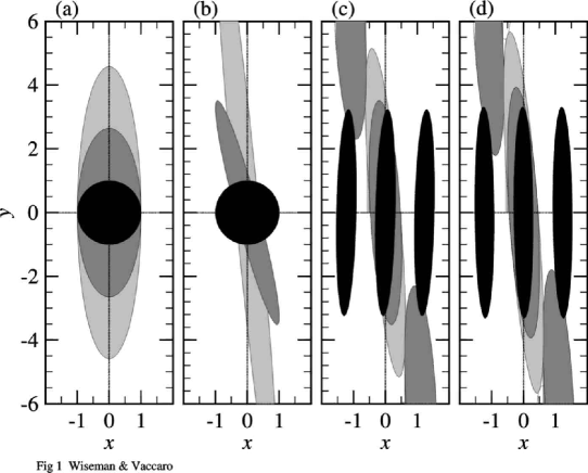
FIG. 1.: The evolution of (initially pure) Gaussian quantum states under the linearized laser master equation for four different cases. The states are represented by the one standard-deviation ellipse of the Wigner function. In the all cases we choose the initial mean location of the state in phase space to be $\bar{x}=\bar{y}=0$, and for the last two we additionally have $\bar{x}=\pm\sqrt{3/2}$. For all four cases the excess phase diffusion is $\nu=0$. For case (a) we have $\chi=0$ and an initially coherent state (which forms the most robust ensemble in this case). For case (b) we have $\chi=50$ and again an initially coherent state. For case (c) we have $\chi=50$ but the initial states are members of the most robust unconstrained ensemble $E^{R}$ for this $\chi$. For case (d) we have $\chi=50$ but the initial states are members of the most robust PR-constrained ensemble $E^{\cal R}$ for this $\chi$. In all cases the black ellipses are for $t=0$, the dark grey ellipses for $t=\tau$ (the appropriate ensemble-averaged survival time), and the light grey ellipses for a still later time. Details of these times are given in the main text.

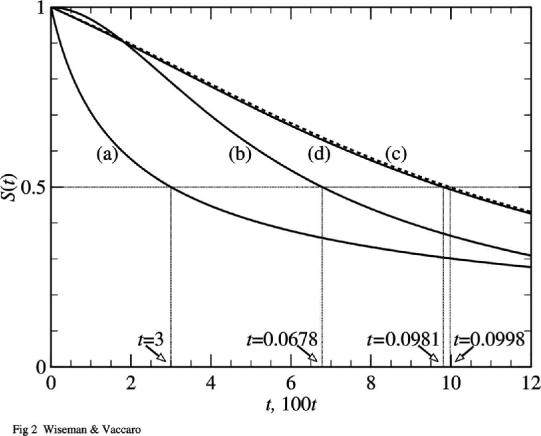
FIG. 2.: The decay of the ensemble-averaged survival probability in time for the four cases represented in Fig. 1. The horizontal axis measures time $t$. For case (a) it is scaled in units of the bare lifetime of the laser mode, and for cases (b), (c), and (d) it is scaled in units 100 times smaller. That is, the survival probabilities actually drop much more quickly for the last three cases.

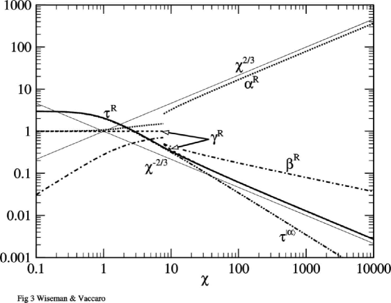
FIG. 3.: The parameters for the most robust unconstrained Gaussian ensemble $E^{\rm R}$ as a function of $\chi$ with $\nu=0$. These parameters are the phase quadrature variance $\alpha^{\rm R}$ (dotted line), the amplitude-quadrature variance $\gamma^{\rm R}$ (dashed line), the covariance $\beta^{\rm R}$ (dash-dot line) and the survival time $\tau^{\rm R}$ for the members of this ensemble. For comparison, we also plot the survival time $\tau^{\left|{\alpha}\right\rangle}$ (dash-dot-dot line) of a coherent state ensemble. Both survival times are in units of the bare lifetime of the laser mode.

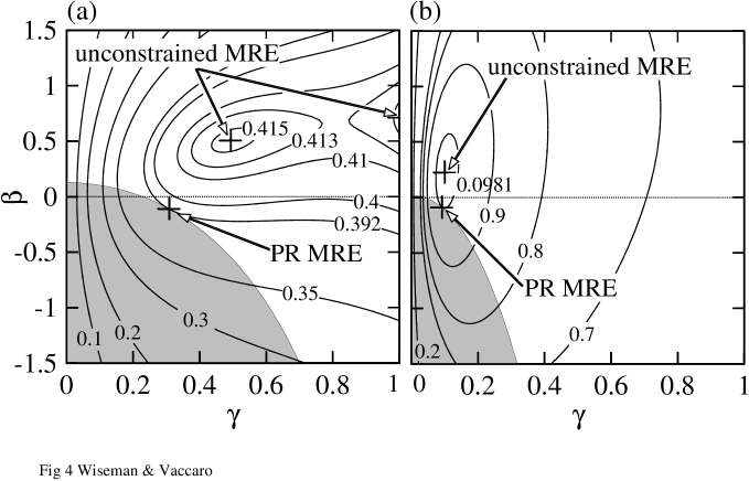
FIG. 4.: Contour plots of the survival time $\tau$ as a function of $\gamma$ and $\beta$. In (a) $\nu=0$ and $\chi=7.7$ and in (b) $\nu=0$ and $\chi=50$. In each plot the heavy curves represent contours of $\tau$ (in units of the bare lifetime of the laser mode) and the shaded region represents states that are physically realizable (PR). Crosses mark the positions of the maximally robust ensembles (MRE).

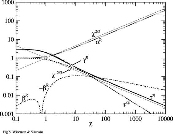
FIG. 5.: The parameters for the ensemble $E^{\cal R}$ arising from the maximally robust unraveling ${\cal R}$ as a function of $\chi$ with $\nu=0$. As in Fig. 3 we plot $\alpha^{\cal R}$ (dotted line), $\gamma^{\cal R}$ (dashed line) and $\pm\beta^{\cal R}$ (dash-dot lines). We also plot the survival time $\tau^{\cal R}$ (solid line) of this ensemble and, for comparison, the survival time $\tau^{\left|{\alpha}\right\rangle}$ (dash-dot-dot line) of a coherent state ensemble. Both of these times are in units of the bare lifetime of the laser mode.

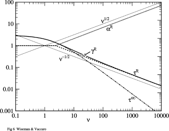
FIG. 6.: The parameters for the ensemble $E^{\cal R}$ arising from the maximally robust unraveling ${\cal R}$ as a function of $\nu$ with $\chi=0$. As in Fig. 3 we plot $\alpha^{\cal R}$ (dotted line), $\gamma^{\cal R}$ (dashed line), and the survival time $\tau^{\cal R}$ (solid line). We do not plot $\beta^{\cal R}$ because it is identically zero. For comparison we also plot the survival time $\tau^{\left|{\alpha}\right\rangle}$ (dash-dot-dotted) of a coherent state ensemble. Both of these times are in units of the bare lifetime of the laser mode.

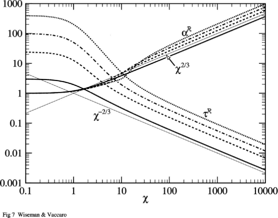
FIG. 7.: The parameters for the ensemble $E^{\cal R}$ arising from the maximally robust unraveling ${\cal R}$ as a function of $\chi$ with $\nu=0$ and for various $\Lambda$. The rising lines are $\alpha^{\cal R}$ and the falling lines are $\tau^{\cal R}$ (in units of the bare lifetime of the laser mode). The values of $\Lambda$ are 0.5 (solid line), 0.2 (dashed line), 0.1 (dash-dot line), and 0.05 (dotted line).

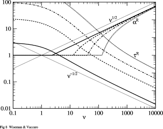
FIG. 8.: The parameters for the ensemble $E^{\cal R}$ arising from the maximally robust unraveling ${\cal R}$ as a function of $\nu$ with $\chi=0$ and for various $\Lambda$. The rising lines are $\alpha^{\cal R}$ and the falling lines are $\tau^{\cal R}$ (in units of the bare lifetime of the laser mode). The values of $\Lambda$ are 0.5 (solid line), 0.2 (dashed line), 0.1 (dash-dot line), and 0.05 (dotted line).

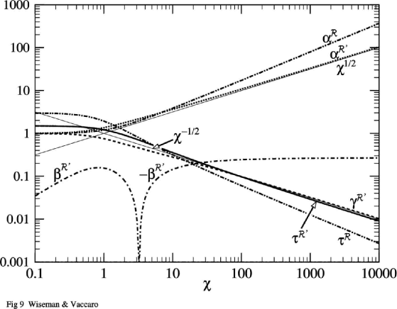
FIG. 9.: Parameters for the maximally robust ensemble for $\nu=0$ as a function of $\chi$ as in Fig. 5 but using purity as a measure of robustness. As in previous figures we plot $\alpha^{\cal R^{\prime}}$ (dotted line), $\gamma^{\cal R^{\prime}}$ (dashed line), $\beta^{\cal R^{\prime}}$ (dash-dot line) and $\tau^{\cal R^{\prime}}$ (solid line). Also shown for comparison are the $\alpha^{\cal R}$ (rising) and $\tau^{\cal R}$ (falling) curves from Fig. 5 as dash-dot-dotted curves. Both times are in units of the bare lifetime of the laser mode.

- [1] H.M. Wiseman, Phys. Rev. A 56, 2068 (1997).
- [2] M. Sargent, M.O. Scully, and W.E. Lamb, Laser Physics (Addison-Wesley, Reading Mass., 1974)
- [3] H.M. Wiseman and J.A. Vaccaro, quant-ph/9906125 (part I).
- [4] J. Gea-Banacloche, in: New Frontiers in Quantum Electrodynamics and Quantum Optics, A.O. Barut, ed., Plenum, New York (1990).
- [5] H.M. Wiseman, Phys. Rev. A 47, 5180 (1993).
- [6] J. Gea-Banacloche, Found. Phys. 28, 531 (1998).
- [7] S.M. Barnett, K. Burnett and J.A. Vaccaro, J. Res. Natl. Inst. Stand. Technol. 101,593 (1996).
- [8] B. Schumacher, Phys. Rev. A 51, 2738 (1995).
- [9] H.M. Wiseman and J.A. Vaccaro, Phys. Lett. A 250, 241 (1998).
- [10] W.H. Zurek, Prog. Theor. Phys. 89, 281 (1993).
- [11] W.H. Zurek, S. Habib, and J.P. Paz, Phys. Rev. Lett 70,1187 (1993).
- [12] M.R. Gallis, Phys. Rev. A 53, 655 (1996).
- [13] Gh.-S. Paraoanu and H. Scutaru Phys. Lett. A 238, 219 (1998).
- [14] L. Diósi and C. Kiefer, Phys. Rev. Lett. 85, 3552 (2000).
- [15] D. Dalvit, J. Dziarmaga, and W.H. Zurek, Phys. Rev. Lett. 86, 373 (2001).
- [16] H.M. Wiseman and Z. Brady, Phys. Rev. A 62, 023805 (2000).
- [17] H.J. Carmichael, An Open Systems Approach to Quantum Optics (Springer-Verlag, Berlin, 1993).
- [18] G. Lindblad, Commun. math. Phys. 48, 199 (1976).
- [19] In Ref. [7] we used the same overlap as in Eq. (9) as a measure of robustness, which, following Ref. [8], we referred to as fidelity. However, we feel that the term survival probability is more appropriate since it embodies the notion of the state to survive over time whereas fidelity embodies the faithful reproduction of a state.
- [20] M. Hillery, R.F. O’Connell, M.O. Scully, and E.P. Wigner, Phys. Rep. 106, 121 (1984).
- [21] N. Gisin and I. Percival, Phys. Lett. A 167, 315 (1992); ibid., J. Phys. A 25, 5677 (1992).
- [22] L. Diósi, Phys. Lett. A 132, 233 (1988).
- [23] J. Anglin, Phys. Rev. Lett. 79, 6 (1997).
- [24] Z. Brady, B.Sc. Honours thesis (Griffith University, 2000).