Stabilization of impurity states in crossed magnetic and electric fields

Abstract

It is shown that the renormalizability of the zero-range interaction in the two-dimensional space is always followed by the existence of a bound state, which is not true for odd-dimensional spaces. A renormalization procedure is defined and the exact retarded Green’s function for electrons moving in two dimensions and interacting with both crossed magnetic and electric fields and an attractive zero-range interaction is constructed. Imaginary parts of poles of this Green’s function determine lifetimes of quasi-bound (resonance) states. It is shown that for some particular parameters the stabilization against decay occurs even for strong electric fields.

I Introduction

The observations of the integer and fractional quantum Hall effects KDP80 ; TSG82 are among the most important discoveries of recent years and have had a profound impact on both applied and fundamental physics. Many aspects of these discoveries are presented in the books edited by Prange and Girvin PG87 and by Das Sarma and Pinczuk SP97 , and in the monographs CP95 ; E00 . From the theoretical point of view the quantum Hall phenomenon is due to the two-dimensional dynamics of electrons moving under the influence of crossed magnetic and electric fields in the presence of impurities. Since the de Broglie wavelength of electrons scattered by impurities is much larger then the interaction range, therefore, it is legitimated to describe a scatterer by a zero-range potential. This, in fact, has been already proposed by Prange P81 shortly after the discovery of the quantum Hall effect, and discussed further in Refs. PJ82 ; JP84 . In his seminal paper Prange studied electron states in two dimensions in perpendicular magnetic and in-plane electric fields in the presence of a single repulsive ’delta-like’ scatterer. Prange’s model, with an attractive zero-range potential and zero electric field, has been reconsidered by Perez and Coutinho PC91 , and by Cavalcanti and de Carvalho CC98 . They showed that the attractive zero-range interaction can be rigorously defined by renormalizing the strength of the $\delta$-function. Such a procedure cannot be develop for a repulsive two-dimensional $\delta$-function (as it will follow shortly), for which an artificial cutoff has to be introduced, as described for instance in Ref. HL99 . The problem of electron scattering by a single impurity represented by a repulsive short-range potential in the presence of both magnetic and electric fields has been further studied from the classical point of view in Ref. BHHP96 , whereas the quantum description has been developed in Ref. HL99 for a repulsive, and in Ref. GM99 for an attractive $\delta$-function potential. Both these quantum analyses show that due to external magnetic and electric fields new long living quasi-bound states appear in the positive part of the energy spectrum, the existence of which appears to be crucial for the explanation of the robustness of the quantum Hall effect P81 ; HL99 .

There has been shown HL99 ; GM99 that in the limit of a very weak electric field the lifetime of these quasi-bound states tends to infinity and grow in a Gaussian way as the electric field tends to zero. This finding, not taking into account, however, the precisely determined functional dependence of the lifetime on the strength of the electric field, agrees with our common understanding of the decay problem in a weak electric field. The aim of this paper is to analyze this problem for strong electric fields. It is usually believed that with an increasing electric field the lifetimes of these quasi-bound states should decrease to zero. It appears, however, that such a behavior is not generally true and that for some particular values of magnetic and electric fields one observes a new phenomenon, the stabilization of these new quasi-bound states. We demonstrate this phenomenon for an attractive $\delta$-function potential considered in Ref. GM99 .

In this paper we use units in which $\hbar=1$.

II Attractive $\delta$-function potential

In this section we shall define the renormalized attractive $\delta$-function potential for one-, two- and three-dimensional cases. To this end let us assume that a quantum system without this interaction is described by the hamiltonian $H_{0}$. We introduce further a regularization of a zero-range potential such that the total hamiltonian is equal to

$$H=H_{0}+\lambda_{\sigma}\delta_{\sigma}(\bm{r}),$$ (1)

in which $\sigma$ is a regularization parameter, $\lambda_{\sigma}$ is a bare coupling constant, and $\delta_{\sigma}(\bm{r})$ tends to the Dirac distribution $\delta(\bm{r})$ in a $d$-dimensional space. Our aim is to construct the retarded Green’s function satisfying the equation

$$(E-H)G^{(+)}(\bm{r},\bm{r}^{\prime};E)=\delta(\bm{r}-\bm{r}^{\prime}),$$ (2)

provided that the range of a regularized potential is very small, i.e., is much smaller than the electron’s de Broglie wavelength or the size of a bound state wave function. This means that in the Lippmann-Schwinger equation

$$G^{(+)}(\bm{r},\bm{r}^{\prime};E)=G_{0}^{(+)}(\bm{r},\bm{r}^{\prime};E)$$

$$+\lambda_{\sigma}\int\text{d}^{d}\bm{r}^{\prime\prime}G_{0}^{(+)}(\bm{r},\bm{r}^{\prime\prime};E)\delta_{\sigma}(\bm{r}^{\prime\prime})G^{(+)}(\bm{r}^{\prime\prime},\bm{r}^{\prime};E),$$ (3)

in which $G_{0}^{(+)}(\bm{r},\bm{r}^{\prime};E)$ is the Green’s function for the hamiltonian $H_{0}$, we can approximate under the integral the full Green’s function $G^{(+)}(\bm{r}^{\prime\prime},\bm{r}^{\prime};E)$ by $G^{(+)}(\bm{0},\bm{r}^{\prime};E)$. This allows to calculate $G^{(+)}(\bm{0},\bm{r}^{\prime};E)$ and to arrive at the following expression for the retarded Green’s function,

$$G^{(+)}(\bm{r},\bm{r}^{\prime};E)=G_{0}^{(+)}(\bm{r},\bm{r}^{\prime};E)$$

$$+\frac{G_{0}^{(+)}(\bm{r},\bm{0};E)G_{0}^{(+)}(\bm{0},\bm{r}^{\prime};E)}{\lambda^{-1}_{\sigma}-\int\text{d}^{d}\bm{r}^{\prime\prime}G_{0}^{(+)}(\bm{0},\bm{r}^{\prime\prime};E)\delta_{\sigma}(\bm{r}^{\prime\prime})}.$$ (4)

In order to proceed further let us choose a particular regularization prescription for which all the space and momentum integrals, that will appear below, can be carried out and expressed in terms of elementary functions, namely,

$$\delta_{\sigma}(\bm{r})=\int\frac{\text{d}^{d}\bm{k}}{(2\pi)^{d}}\exp(\text{i}\bm{k}\cdot\bm{r}-\sigma^{2}\bm{k}^{2}).$$ (5)

Let us also assume for a moment that $H_{0}$ describes free electrons of a reduced mass $m^{*}$. For such a hamiltonian the retarded Green’s function adopts the form

$$G_{0}^{(+)}(\bm{r},\bm{r}^{\prime};E)=-\text{i}\int_{0}^{\infty}\text{d}t\text{e}^{\text{i}(E+\text{i}\varepsilon)t}\int\frac{\text{d}^{d}\bm{k}}{(2\pi)^{d}}\exp\biggl{(}\text{i}\bm{k}\cdot(\bm{r}-\bm{r}^{\prime})-\text{i}\frac{\bm{k}^{2}}{2m^{*}}t\biggr{)},$$ (6)

in which $\varepsilon$ is an infinitesimally small positive real number. Thus, after performing the Gauss integration over $\bm{k}$, the denominator in eq. (4) becomes

$$D(E)=\lambda^{-1}_{\sigma}+\text{i}\biggl{(}\frac{m^{*}}{2\pi\text{i}}\biggr{)}^{d/2}\int_{0}^{\infty}\text{d}t\frac{\text{e}^{\text{i}(E+\text{i}\varepsilon)t}}{(t-2\text{i}m^{*}\sigma^{2})^{d/2}}.$$ (7)

As we see, for $d=1$ the last integral exists for $\sigma=0$, i.e., there is no need for the renormalization of a coupling constant $\lambda_{\sigma}$. On the other hand, for $d>1$ the integral in the equation above diverges for small $t$ in the limit of a vanishing regularization parameter $\sigma$. It can be shown, however, that the divergent part of this integral can be absorbed into the bare coupling constant $\lambda_{\sigma}$. To this end let us consider in the beginning the case of $d=2$. Integrating by parts we end up in the limit of vanishing $\sigma$ with

$$D(E)=\lambda_{R}^{-1}+\frac{m^{*}}{2\pi}\biggl{(}\ln(\text{i})-\text{i}E\int_{0}^{\infty}\text{d}t\text{e}^{\text{i}(E+\text{i}\varepsilon)t}\ln(t/t_{0})\biggr{)},$$ (8)

where $t_{0}$ is an arbitrary positive real number of the same dimensionality as $t$, introduced only for dealing with a dimensionless argument of the logarithm function, and $\lambda_{R}$ is the renormalized coupling constant

$$\lambda_{R}^{-1}=\lim_{\sigma\rightarrow 0}\Bigl{[}\lambda_{\sigma}^{-1}-\frac{m^{*}}{2\pi}\ln\Bigl{(}\frac{2m^{*}\sigma^{2}}{t_{0}}\Bigr{)}\Bigr{]}.$$ (9)

As it follows from the equation above the bare coupling constant $\lambda_{\sigma}$ has to be negative in order to carry out the renormalization procedure. Hence, the zero-range limit exists only for an attractive interaction. Performing the remaining integration we finally arrive at

$$D(E)=\lambda_{R}^{-1}+\frac{m^{*}}{2\pi}\ln\biggl{(}\frac{\text{e}^{-\gamma}}{-Et_{0}}\biggr{)},$$ (10)

where $\gamma$ is the Euler’s constant. Since the energy of a bound state, $E_{B}<0$, supported by this interaction is determined by the zero of $D(E)$, therefore

$$E_{B}=-\frac{1}{t_{0}}\text{e}^{-\gamma+2\pi/\lambda_{R}m^{*}}.$$ (11)

As one sees, the expression above is always negative, independently weather the renormalized coupling constant is negative or positive. This means that the zero-range potential in two-dimensional space always supports one bound state. Combining (10) with (11) we arrive at the following expression for the denominator $D(E)$,

$$D(E)=\frac{m^{*}}{2\pi}\ln\biggl{(}\frac{E_{B}}{E}\biggr{)},$$ (12)

in which an artificial parameter $t_{0}$ does not appear any more.

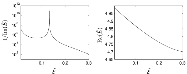
Figure 1: Presents the dependence of the lifetime $\tau=-1/\text{Im}(\tilde{E})$ and the real part of $\tilde{E}$ on the scaled electric field $\tilde{\mathcal{E}}$ for an impurity which supports one bound state of energy $\tilde{E}_{B}=-6.4$. For $\tilde{\mathcal{E}}=0.132$ we observe the stabilization of a resonance state located just below the third Landau level.

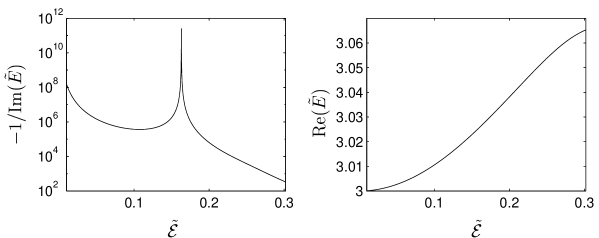
Figure 2: The same as in Fig. 1 but for $\tilde{E}_{B}=-2.8$. The stabilization occurs for $\tilde{\mathcal{E}}=0.163$ for a resonance state located just above the second Landau level.

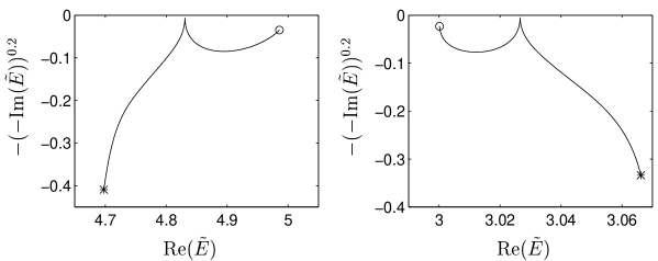
Figure 3: Shows the trajectories of two resonances considered in Figs. 1 and 2 in the complex energy plane. For the visual purpose the imaginary part is raised to the power $1/5$. The left frame corresponds to the binding energy $\tilde{E}_{B}=-6.4$ and the right one to $\tilde{E}_{B}=-2.8$. The circle marks the minimum value $\tilde{\mathcal{E}}=0.01$, whereas the asterisk indicates the maximum value $\tilde{\mathcal{E}}=3.1$. The stabilization occurs for $\tilde{\mathcal{E}}=0.132$, $\text{Re}(\tilde{E})=4.83$, $\text{Im}(\tilde{E})=-0.111\times 10^{-10}$ and $\tilde{\mathcal{E}}=0.163$, $\text{Re}(\tilde{E})=3.0266$, $\text{Im}(\tilde{E})=-0.398\times 10^{-11}$, respectively.

The existence of a bound state for a zero-range interaction, irrespectively of the sign of a renormalized coupling constant, can only happen for $d=2$. In order to show this let us consider the case of $d=3$. Now we do not need to introduce $t_{0}$ and end up with

$$D(E)=\lambda_{R}^{-1}+\frac{m^{*}}{2\pi}\sqrt{-2m^{*}E},$$ (13)

where the renormalized coupling constant is equal to

$$\lambda_{R}^{-1}=\lim_{\sigma\rightarrow 0}\Bigl{(}\lambda_{\sigma}^{-1}+\frac{m^{*}}{2\pi^{3/2}\sigma}\Bigr{)}.$$ (14)

Hence, it is clearly seen that again the renormalization procedure can be only performed for a negative bare coupling constant. Nevertheless, contrary to the two-dimensional case, a bound state exists only for a negative renormalized coupling constant $\lambda_{R}$. A similar situation occurs for the one-dimensional $\delta$-function potential supporting one bound state just for negative coupling constants (renormalized and bare coupling constants are equal here and amount to $-\sqrt{2|E_{B}|/m^{*}}$).

Summarizing, for the two-dimensional zero-range interaction the renormalizability is followed by the existence of a bound state, irrespectively of the sign of the renormalized coupling constant. In our further discussion we shall limit ourselves to the two-dimensional renormalizable zero-range interaction. Let us also note in closing this section that the zero-range potential for an arbitrary dimensional space has been studied by Wódkiewicz W90 who also emphasized the difference between odd and even dimensions.

III Quasi-bound states in crossed magnetic and electric fields

We can now include into our two-dimensional model external magnetic and electric fields. For this we need the exact form of the retarded Green’s function for the hamiltonian

$$H_{0}=\frac{1}{2m^{*}}\Bigl{(}-\text{i}\bm{\nabla}-e\bm{A}(\bm{r})\Bigr{)}^{2}-e\bm{\mathcal{E}}\cdot\bm{r}.$$ (15)

Let us assume that electrons move in the $xy$-plane, the magnetic field $\bm{\mathcal{B}}$ is perpendicular to this plane and the electric field $\bm{\mathcal{E}}$ points into the $x$-direction. For such a geometry and for the vector potential in the symmetric gauge, i.e. $\bm{A}=\frac{1}{2}\bm{\mathcal{B}}\times\bm{r}$,

$$H_{0}=\frac{1}{2m^{*}}\Bigl{[}\Bigl{(}-\text{i}\partial_{x}+\frac{e{\mathcal{B}}}{2}y\Bigr{)}^{2}+\Bigl{(}-\text{i}\partial_{y}-\frac{e{\mathcal{B}}}{2}x\Bigr{)}^{2}\Bigr{]}-e{\mathcal{E}}x,$$ (16)

and the Green’s function adopts the form

$$G_{0}^{(+)}(\bm{r},\bm{r}^{\prime};E)=-\frac{m^{*}\omega}{4\pi}\int_{0}^{\infty}\text{d}t\frac{\text{e}^{\text{i}(E+\text{i}\varepsilon)t}}{\sin\frac{\omega t}{2}}\exp\biggl{[}\frac{\text{i}m^{*}\omega}{4}\bigl{(}(x-x^{\prime})^{2}+(y-y^{\prime})^{2}\bigr{)}\cot\frac{\omega t}{2}$$

$$+\frac{\text{i}m^{*}\omega}{2}(xy^{\prime}-x^{\prime}y)+\frac{\text{i}e\mathcal{E}t}{2}(x+x^{\prime})+\frac{\text{i}e{\mathcal{E}}}{\omega}\Bigl{(}\frac{\omega t}{2}\cot\frac{\omega t}{2}-1\Bigr{)}\Bigl{(}-y+y^{\prime}+\frac{e{\mathcal{E}}t}{2m^{*}\omega}\Bigr{)}\biggr{]},$$ (17)

with $\omega=|e|{\mathcal{B}}/m^{*}$ being the cyclotron frequency. Since lifetimes of quasi-bound states are determined by poles of the Green’s function, therefore, we shall concentrate in our further discussion on the denominator in eq. (4). One can find that in this particular case $D(E)$ can be expressed as follows,

$$D(E)=\lambda_{\sigma}^{-1}+\frac{m^{*}\omega}{4\pi}\int_{0}^{\infty}\text{d}t\frac{\text{e}^{\text{i}(E+\text{i}\varepsilon)t}}{\sin\frac{\omega t}{2}-\text{i}m^{*}\omega{\sigma}^{2}\cos\frac{\omega t}{2}}\exp\Biggl{[}\frac{\text{i}t}{2m^{*}}\Bigl{(}\frac{e{\mathcal{E}}}{\omega}\Bigr{)}^{2}\Bigl{(}\frac{\omega t}{2}\cot\frac{\omega t}{2}-1\Bigr{)}$$

$$-{\sigma}^{2}\Bigl{(}\frac{e{\mathcal{E}}}{\omega}\Bigr{)}^{2}\frac{\bigl{(}\frac{\omega t}{2}\bigr{)}^{2}+\bigl{(}\frac{\omega t}{2}\cot\frac{\omega t}{2}-1\bigr{)}^{2}}{1-\text{i}m^{*}\omega{\sigma}^{2}\cot\frac{\omega t}{2}}\Biggl{]},$$ (18)

where the integral above diverges logarithmically for small values of $t$ in the zero-range limit. However, as we have proved it in the previous section, this singularity can be removed by combining the divergent term with the bare coupling constant $\lambda_{\sigma}$.

For our further analysis it is convenient to introduce dimensionless variables, in which the length is measure in the units of $1/\sqrt{m^{*}\omega}$, whereas the electric field and the energy are scaled as $\tilde{\mathcal{E}}=|e|{\mathcal{E}}/\sqrt{m^{*}\omega^{3}}$ and $\tilde{E}=2E/\omega$, respectively. Changing the integration variable to $s=\omega t/2$ we obtain finally for $\sigma\rightarrow 0$,

$$D(E)=\frac{m^{*}}{2\pi}\biggl{[}\ln\biggl{(}\frac{\tilde{E}_{B}}{\tilde{E}}\biggr{)}+\int_{0}^{\infty}\text{d}s\text{e}^{\text{i}(\tilde{E}+\text{i}\varepsilon)s}\Biggl{(}\frac{\exp\bigl{(}\text{i}{\tilde{\mathcal{E}}}^{2}s(s\cot s-1)\bigr{)}}{\sin s}-\frac{1}{s}\Biggr{)}\biggr{]}.$$ (19)

We shall demonstrate now that even in strong electric fields one can observe long living quasi-bound states. This nonperturbative result follows from the numerical determination of zeros of $D(E)$. It appears that for some particular values of the electric field and the binding energy there exist zeros of (19) with very small imaginary parts, although real parts remain positive. This phenomenon, which we call the stabilization, is presented in Figs. 1, 2 and 3. In Figs. 1 and 2 we draw the dependence of lifetimes, $\tau=-(2\text{Im}(E))^{-1}=-(\omega\text{Im}(\tilde{E}))^{-1}$, and real parts of $E$, $\text{Re}(E)=\frac{\omega}{2}\text{Re}(\tilde{E})$, in units of $\omega^{-1}$ and $\omega/2$, respectively. We see that with the increasing electric field the lifetime initially decreases, which is a commonly accepted result. We observe, however, that at a particular value for the electric field the lifetime starts increasing, approaches its maximum, and then monotonically decreases. In both presented cases the real part of $E$ remains positive and is just below the third Landau level of energy $5\omega/2$ or above the second one of energy $3\omega/2$. In Fig. 3 we show the position of these poles of the Green’s function in the complex energy plane. Only for the visual purpose the imaginary part is raised to the power $1/5$. We see that with an increasing electric field the poles in the beginning depart from the real axis, but afterward start approaching it, reach minimum for the absolute value of the imaginary part of $E$ (which appears to be almost equal to zero within the accuracy of our numerical calculation) and then again migrate downward. Such an unexpected non-monotonic behavior happens for some particular values of the binding energies as well as the applied fields. At this point let us only mention that estimations of magnetic and electric fields show that they can be generated easily in experimental setups.

What we have checked in our numerical investigations is that the stabilization occurs only for states which are close to the excited Landau levels and does not appear for states near the first Landau level. Indeed, for very small electric fields resonances considered in this paper approach the second and the third Landau levels, i.e., the excited ones. This appears to be a general rule that the electric field generates new resonance states in a close vicinity of excited Landau levels. These states differ from the ones considered by Prange P81 and reinvestigated by Cavalcanti and de Carvalho CC98 . In their case, when the electric field is switched off, the point interaction modifies only Landau states with the vanishing angular momentum, because only for these states the wavefunction does not vanish at the origin. The states with a non-zero angular momentum, i.e., the vortex Landau states, for which the wavefunctions explicitly depend on the polar angle $\varphi$ and vanish at the origin, are not affected by a point interaction. The situation changes if a small electric field is applied. Then the vortex Landau states acquire small contributions which do not vanish at the origin, as follows for instance from perturbation theory. Hence, the interaction with a contact potential does not vanish, and apart from the well-known states considered previously P81 ; CC98 new resonance states emerge close to the excited Landau levels. These are the states for which the stabilization takes place. Since the wavefunction of them for small electric fields is predominantly composed of the vortex Landau states of non-zero angular momentum, therefore, one can call them the vortex resonance states. This fact suggests that the stabilization presented in this paper is due to the angular motion of electrons around the impurity, as it also happens in the classical considerations for a repulsive potential BHHP96 . The analysis presented above can be applied to weak electric fields. For strong nonperturbative electric fields we can rather rely on the exact numerical analysis of this problem with the hope that the picture above still remains valid. However, the almost total suppression of ionization rates for some particular values of the electric field hardly can be explained only in terms of classical physics and we expect that its origin is due to complicated quantum interference effects which can only be studied numerically.

- (1) K. von Klitzing, G. Dorda, and M. Pepper, Phys. Rev. Lett. 45, 494 (1980).
- (2) D. C. Tsui, H. L. Stormer, and A. C. Gossard, Phys. Rev. Lett. 48, 1559 (1982).
- (3) R. E. Prange and S. M. Girvin (eds.), The Quantum Hall Effect, (Springer, New York, 1987).
- (4) S. Das Sarma and A. Pinczuk (eds.), Perspectives in Quantum Hall Effects, (John Wiley & Sons, New York, 1997).
- (5) T. Chakraborty and P. Pietiläinen, The Quantum Hall Effects. Fractional and Integral, (Springer, Berlin Heidelberg, 1995), 2nd Ed.
- (6) Z. F. Ezawa, Quantum Hall Effects. Field Theoretical Approach and Related Topics, (World Scientific, Singapore, 2000).
- (7) R. E. Prange, Phys. Rev. B 23, 4802 (1981).
- (8) R. E. Prange and R. Joynt, Phys. Rev. B 25, 2943 (1982).
- (9) R. Joynt and R. E. Prange, Phys. Rev. B 29, 3303 (1984).
- (10) F. Perez and F. A. B. Coutinho, Am. J. Phys. 59, 52 (1991).
- (11) R. M. Cavalcanti and C. A. A. de Carvalho, J. Phys. A 31, 2391 (1998).
- (12) E. H. Hauge and J. M. J. van Leeuwen, Physica A 268, 525 (1999).
- (13) N. Berglund, A. Hansen, E. H. Hauge, and J. Piasecki, Phys. Rev. Lett. 77, 2149 (1996).
- (14) S. Gyger and P. A. Martin, J. Math. Phys. 40, 3275 (1999).
- (15) K. Wódkiewicz, Phys. Rev. A 43, 68 (1991).