Geometric Quantum Computation on Solid-State Qubits

Abstract

Geometric quantum computation is a scheme to use non-Abelian Holonomic operations rather than the conventional dynamic operations to manipulate quantum states for quantum information processing. Here we propose a geometric quantum computation scheme which can be realized with current technology on nanoscale Josephson-junction networks, known as a promising candidate for solid-state quantum computer.

I Introduction

The elementary units of quantum information processing are quantum two-state systems, called quantum bits or “qubits”. Unlike a classical bit, a qubit can be in any superposition $\alpha|\bar{0}\rangle+\beta|\bar{1}\rangle$ (with $\alpha$ and $\beta$ arbitrary complex numbers satisfying the normalization condition $|\alpha|^{2}+|\beta|^{2}=1$) of the computational basis states $|\bar{0}\rangle$ and $|\bar{1}\rangle$. A qubit needs not only to preserve quantum coherence for a sufficiently long time but also to allow an adequate degree of controllability. Among a number of ideas proposed so far to realize qubits, the ones based on solid-state devices have attracted interest due to the scalability for massive information processing, which can make a quantum computer of practical value Averin01a .

Another crucial element of quantum information processing is the ability to perform quantum operations on qubits in a controllable way and with sufficient accuracy. In most proposed schemes such quantum operations are unitary, and conventionally have been achieved based on quantum dynamics governed by the Schrödinger equation.

Recently, it has been proposed that controllable quantum operations can be achieved by a novel geometric principle as well Zanardi99a ; Pachos00a . When a quantum system undergoes an adiabatic cyclic evolution, it acquires a non-trivial geometric operation called a holonomy. Holonomy is determined entirely by the geometry of the cyclic path in the parameter space, independent of any detail of the dynamics. If the eigenspace of the Hamiltonian in question is non-degenerate, the holonomy reduces to a simple phase factor, a Berry phase. Otherwise, it becomes a non-Abelian unitary operation, i.e., a non-trivial rotation in the eigenspace. It has been shown that universal quantum computation is possible by means of holonomies only Zanardi99a ; Pachos00a . Further, holonomic quantum computation schemes have intrinsic tolerance to certain types of computational errors Preskill99a ; Ellinas01a .

A critical requirements for holonomies is that the eigenspace should be preserved throughout the adiabatic change of parameters, which is typically fulfilled by symmetry Wilczek84a . It is non-trivial to devise a physical system with a proper eigenspace which will serve as a computational space. Recently a scheme for geometric quantum computation with nuclear magnetic resonance was proposed and demonstrated experimentally Jones00a . A similar scheme was proposed on superconducting nanocircuits Falci00a . In these schemes, however, geometrically available was only Abelian Berry phase, and additional dynamic manipulations were required for universal quantum computation. A scheme based solely on holonomies has been proposed for quantum optical systems Pachos00b . However, it relies on nonlinear optics, which may make this scheme less practical. More recently, another holonomic quantum computation scheme has been proposed for trapped ions DuanLM01a . Supposedly, it is the only experimentally feasible scheme proposed so far for holonomic computation. Here we propose a scheme for holonomic quantum computation on nanoscale Josephson networks, known as a promising candidate for solid-state quantum computer Makhlin99a ; Nakamura99a ; Mooij99a . It relies on tunable Josephson junction and capacitive coupling, which are already viable with current technology.

II Josephson Charge Qubits

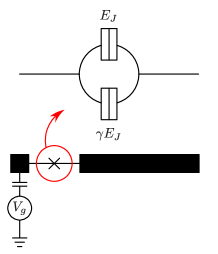
Figure 1: A schematic of a “Josephson charge qubit”. The cross denotes a tunable Josephson junction, which consists of two parallel tunnel junctions (upper panel). The strength of the effective Josephson coupling is tuned by flux threading the loop. The gate voltage $V_{g}$ controls the induced charge on the box.

A “Josephson (charge) qubit” Makhlin99a ; Nakamura99a can be realized by a small superconducting grain (a Cooper-pair box) of size $\sim 100\mathrm{nm}$, coupled to a large superconducting charge reservoir or another Cooper-pair box via a Josephson junction, see Fig. 1. The computational bases are encoded in two consecutive charge states $|\bar{0}\rangle\to|0\rangle$ and $|\bar{1}\rangle\to|1\rangle$ with $|n\rangle$ denoting a state with $n$ excess Cooper pairs on the box. States with more (or less) Cooper pairs are suppressed due to the strong Coulomb repulsion (the gate-induced charge $2en_{g}$ is tuned close to $1/2\mod 1$), characterized by the charging energy $E_{C}=(2e)^{2}/2C$ (with $C$ the total capacitance of the box). Excitation of quasiparticles is also ignored assuming sufficiently low temperature. The tunneling of Cooper pairs across the junction, characterized by the Josephson coupling energy $E_{J}$ ($\ll{}E_{C}$), allows coherent superposition of the charge states $|0\rangle$ and $|1\rangle$. A tunable junction is attained by two parallel junctions making up a SQUID (superconducting quantum interference device) with a magnetic flux $\Phi$ threading through the loop, see upper panel of Fig. 1 Tinkham96a . Namely, in the two-state approximation, the Hamiltonian is written in terms of the Pauli matrices $\sigma^{z}$ and $\sigma^{\pm}=\frac{1}{2}\left(\sigma^{x}\pm i\,\sigma^{y}\right)$ as Falci00a ; Makhlin99a

$$H=-\frac{1}{2}h(n_{g})\sigma^{z}-\frac{1}{2}\left[J(\phi)\sigma^{+}+J^{*}(\phi)\sigma^{-}\right]$$ (1)

where $h(n_{g})=E_{C}(2n_{g}-1)$, $J(\phi)$ is the effective Josephson coupling of the tunable junction (i.e. SQUID), and $\phi=\pi\Phi/\Phi_{0}$ (we assume that $|\phi|\leq\pi/2$) with $\Phi_{0}=hc/2e$ the superconducting flux quantum. Given Josephson energies $E_{J}$ and $\gamma{}E_{J}$ ($\gamma>0$) of the two parallel junctions on a SQUID loop, the magnetic flux gives rise to a phase shift $\alpha(\phi)$ as well as an amplitude modulation $A(\phi)$ of the effective Josephson coupling $J(\phi)=2E_{J}\,A(\phi)e^{-i\alpha(\phi)}$. $A(\phi)$ and $\alpha(\phi)$ are given by Falci00a

$$A(\phi)=\sqrt{(1-\gamma)^{2}/4+\gamma\cos^{2}\phi}$$ (2)

and

$$\tan\alpha(\phi)=\frac{1-\gamma}{1+\gamma}\tan\phi\,,$$ (3)

respectively. It is worth noticing that for identical junctions ($\gamma=1$), (i) there is no phase modulation [$\alpha(\phi)=0$] and (ii) the effective Josephson coupling can be turned off completely [$J(\phi)=0$] at $\phi=\pi/2$. In what follows, some tunable junctions have $\gamma=1$ and others $\gamma\neq 1$ depending on their roles for the system.

Below we will demonstrate that one can obtain the three unitary operations, $U_{Z}(\varphi)=\exp\left(i\varphi|\bar{1}\rangle\langle\bar{1}|\right)$ (phase shift), $U_{X}(\varphi)=\exp\left(i\varphi\sigma^{x}\right)$ (rotation around $x$ axis), and $U_{CZ}(\varphi)=\exp\left(+i\varphi|\bar{1}\bar{0}\rangle\langle\bar{1}\bar{0}|\right)$ (controlled phase shift), on an arbitrary qubit or pair of qubits, using geometric manipulations only. It is known that these unitary operations form a universal set of gate operations for quantum computation Lloyd95a ; DuanLM01a . Since the charge degrees of freedom is used in the present scheme, the state preparation and the state readout, which are another important procedures required for quantum computation, can be achieved using the same methods used in dynamical schemes Makhlin99a .

III Elementary Gates

Before demonstrating the geometric implementation of elementary gates, we suggest a prototype Hamiltonian which reveals the proper symmetry for geometric manipulations in question. All the Hamiltonians considered in this paper share the following common structure:

$$H=\epsilon|\hat{0}\rangle\langle\hat{0}|-\frac{1}{2}\sum_{i=1}^{N}\left(\Omega_{i}|\hat{i}\rangle\langle\hat{0}|+\Omega_{i}^{*}|\hat{0}\rangle\langle\hat{i}|\right)\,.$$ (4)

Here $\Omega_{i}$ is the transition amplitude from the state $|\hat{0}\rangle$ to $|\hat{i}\rangle$ and $\epsilon$ is the energy of the state $|\hat{0}\rangle$ measured from the degenerate energy of the states $|\hat{i}\rangle$ ($i=1,\ldots,N$). For our consideration below, one may regard the state vector $|\hat{i}\rangle$ ($i=0,1,\ldots,N$) represent, e.g., an excess Cooper pair on the $i$th superconducting box, see Fig. 2 (a). $|\hat{i}\rangle$ may also represent electronic levels in atoms such as discussed in Ref. DuanLM01a, .

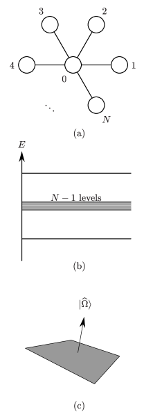
Figure 2: (a) A schematic representation of the prototype model, Eq. (4), which has a proper degenerate eigenspace for geometric quantum computation. (b) The degenerate level structure of the model. (c) The structure of the corresponding Hilbert space, in which the degenerate subspace is always perpendicular to $|\Omega\rangle$.

As one changes the parameters $\Omega_{i}$, the Hamiltonian in Eq. (4) preserves the $(N{-}1)$-dimensional degenerate subspace. This can be clearly seen by defining $|\widehat{\Omega}\rangle\equiv\Omega^{-1}\sum_{i=1}^{N}\Omega_{i}|\hat{i}\rangle$ with $\Omega^{2}\equiv\sqrt{|\Omega_{1}|^{2}+\cdots+|\Omega_{N}|^{2}}$, and rewriting $H$ as

$$H=\epsilon|\hat{0}\rangle\langle\hat{0}|-\frac{1}{2}\Omega\left(|\widehat{\Omega}\rangle\langle\hat{0}|+|\hat{0}\rangle|\widehat{\Omega}\rangle\right)\,.$$ (5)

The Hamiltonian in Eq. (5) corresponds to a particle in a (biased) double-well potential in the tight-binding approximation. Therefore, it has two eigenstates $|\lambda_{\pm}\rangle=\frac{1}{\sqrt{2}}(|\widehat{\Omega}\rangle\mp|\hat{0}\rangle)$ with energies $\lambda_{\pm}=\frac{1}{2}(\epsilon\pm\sqrt{\Omega^{2}+\epsilon^{2}})$. The other $N-1$ levels out of $N+1$ form a degenerate subspace $\mathcal{E}_{N-1}$ with energy $0$, which we will use later for a computational subspace, see Fig. 2 (b). Notice that the degenerate eigenspace $\mathcal{E}_{N-1}$ is always perpendicular both to $|\hat{0}\rangle$ and $|\widehat{\Omega}\rangle$; as the parameters $\Omega_{i}$ change, $|\widehat{\Omega}\rangle$ rotates in the Hilbert space, and the eigenspace $\mathcal{E}_{N-1}$ is attached rigidly, perpendicular to $|\widehat{\Omega}\rangle$, see Fig. 2 (c).

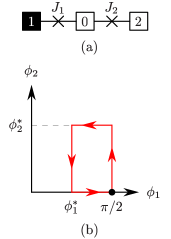
Figure 3: Configuration for the phase-shift operation $U_{Z}$. Throughout the work, computational bases are encoded in the solid boxes and empty boxes serve as ancilla qubits.

We first show how to get the unitary operation $U_{Z}$ geometrically. We consider three Cooper-pair boxes coupled in series as shown in Fig. 3. The first (solid) box encodes the computational bases while the second and third (empty) boxes serve as “ancilla” qubits. The Hamiltonian is given by [see Eq. (1)]

$$H=-\frac{1}{2}\sum_{n=1}^{2}\left(J_{n}\sigma_{n}^{+}\sigma_{0}^{-}+h.c.\right)-\frac{1}{2}h\,\sigma_{0}^{z}$$ (6)

with $h.c.$ meaning the Hermitian conjugate. Comparing Eq. ((6)) with the prototype Hamiltonian in Eq. (4), noticed are following correspondences: $|\hat{0}\rangle\to|100\rangle_{012}$ ($|100\rangle_{123}$ is short for $|1\rangle_{0}|0\rangle_{1}|0\rangle_{2}$), $|\hat{1}\rangle\to|010\rangle_{012}$, $|\hat{2}\rangle\to|001\rangle_{012}$, $|\hat{3}\rangle\to|000\rangle_{012}$, $\Omega_{1}\to J_{1}$, $\Omega_{2}\to J_{2}$, and $\Omega_{3}=0$. From this [or direct diagonalization of the Hamiltonian Eq. (6), of course], one can see that the two states

$$|\lambda_{1}\rangle=J_{2}^{*}|010\rangle_{012}-J_{1}^{*}|001\rangle_{012}$$ (7)

(not normalized) and

$$|\lambda_{2}\rangle=|000\rangle_{012}$$ (8)

form a degenerate subspace with energy $-h/2$, which is preserved during the change of $J_{1}$ and $J_{2}$ (equivalently $\phi_{1}$ and $\phi_{2}$). Since the computational basis is only encoded in the “true” qubit (box 1), the total wave function $|\Psi\rangle$ of the logical block should be initially prepared in a separable state with respect to the true qubit and the ancilla qubits, $|\Psi\rangle=|\psi\rangle_{1}\otimes|\psi^{\prime}\rangle_{02}$. In other words, one should be able to turn off at will the tunable junction 1, which should therefore be made of identical parallel junctions ($\gamma_{1}=1$), see Eqs. (2) and (3). After a cyclic evolution of the parameters $\phi_{1}$ and $\phi_{2}$ along a closed loop starting and ending at the point with $\phi_{1}=\pi/2$ (i.e., $J_{1}=0$), the state $|\lambda_{1}\rangle$ acquires the Berry phase Berry84a . For example, along the loop depicted in Fig. 3 (b), the Berry phase is given by

$$\varphi_{B}=\frac{1-\gamma_{2}^{2}}{4}\int_{0}^{\phi_{2}^{*}}{d\phi_{2}}\;\left[\frac{1}{\cos^{2}\phi_{1}^{*}+A_{2}^{2}(\phi_{2})}-\frac{1}{A_{2}^{2}(\phi_{2})}\right]\,.$$ (9)

(The Berry phase vanishes if $\gamma_{2}=1$ as expected Berry84a .) The state $|\lambda_{2}\rangle$ remains unchanged. Therefore, the cyclic evolution amounts to $U_{Z}(\varphi_{B})$.

Here it should be emphasized that although used is the Abelian Berry phase, the degenerate structure is crucial. The dynamic phases acquired by $|\lambda_{1}\rangle$ and $|\lambda_{2}\rangle$ are the same and result in a trivial global phase. In recently proposed schemes Jones00a ; Falci00a , which have no degenerate structure, at least one dynamic manipulation was unavoidable to remove the dynamically accumulated phases. Another point to be stressed is that the phase shift $\alpha_{2}(\phi_{2})$ in the effective Josephson coupling $J_{2}(\phi_{2})$ is indispensable for the Berry phase.

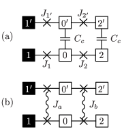
Figure 4: (a) Configuration for the two-qubit gate $U_{CZ}$. (b) Effective “joint-tunnel” coupling (crossed wiggly lines) resulting from the capacitive coupling in (a).

The two-qubit gate operation $U_{CZ}$ can be realized geometrically using capacitive coupling. As shown in Fig. 4 (a), the ancilla qubits on different three-box systems are coupled in parallel via capacitors with capacitance $C_{c}$. It is known ChoiMS98f ; Shimada00a ; Averin91a ; Matters97a that for $C_{c}$ sufficiently larger than the self-capacitance $C$ of each box, the states $|01\rangle_{00^{\prime}}$ and $|10\rangle_{00^{\prime}}$ are strongly favored over the states $|00\rangle_{00^{\prime}}$ and $|11\rangle_{00^{\prime}}$, and the same for boxes $2$ and $2^{\prime}$ (recall that $n_{g}\approx{}1/2$ for each box). This effectively leads to a “joint tunneling”, see Fig. 4 (b): Tunneling of a charge from box $1$ to $0$ should be accompanied by tunneling of another charge from $0^{\prime}$ to $1^{\prime}$. The joint-tunneling amplitudes are given by $J_{a}\approx{}4J_{1}J_{1^{\prime}}^{*}/E_{C}$ and $J_{b}\approx{}4J_{2}J_{2^{\prime}}^{*}/E_{C}$ ChoiMS98f . Then the total Hamiltonian has the form

$$H=-\frac{1}{2}\left[J_{a}\left(\sigma_{1}^{+}\sigma_{0}^{-}\right)\left(\sigma_{1^{\prime}}^{-}\sigma_{0^{\prime}}^{+}\right)+h.c.\right]\\ -\frac{1}{2}\left[J_{b}\left(\sigma_{2}^{+}\sigma_{0}^{-}\right)\left(\sigma_{2^{\prime}}^{-}\sigma_{0^{\prime}}^{+}\right)+h.c.\right]-\frac{1}{2}h\left[\sigma_{0}^{z}-\sigma_{0^{\prime}}^{z}\right]\,.$$ (10)

In analogy with Eqs. (4) and (6), the above Hamiltonian has an eigenspace containing the four degenerate states

$$|\lambda_{00}\rangle=|00\rangle_{11^{\prime}}\otimes|0101\rangle_{00^{\prime}22^{\prime}}\,,$$ (11)

$$|\lambda_{01}\rangle=|01\rangle_{11^{\prime}}\otimes|0101\rangle_{00^{\prime}22^{\prime}}\,,$$ (12)

$$|\lambda_{11}\rangle=|11\rangle_{11^{\prime}}\otimes|0101\rangle_{00^{\prime}22^{\prime}}\,,$$ (13)

and

$$|\lambda_{10}\rangle=J_{b}^{*}|{10}\rangle_{11^{\prime}}\otimes|0101\rangle_{00^{\prime}22^{\prime}}-J_{a}^{*}|01\rangle_{11^{\prime}}\otimes|0110\rangle_{00^{\prime}22^{\prime}}$$ (14)

(not normalized) with energy $-h$. As in the previous case [see discussions below Eq. (8)], it is assumed that the tunable junctions $J_{1}$ and $J_{1^{\prime}}$ are composed of identical parallel junctions ($\gamma_{1}=\gamma_{1^{\prime}}=1$), while $\gamma_{2}\neq 1$ and $\gamma_{2^{\prime}}\neq 1$. One can fix $\phi_{1^{\prime}}=\phi_{2^{\prime}}=0$ and change the parameters $\phi_{1}$ and $\phi_{2}$ along a closed loop starting from the point with $\phi_{1}=\pi/2$ ($J_{1}=J_{a}=0$). Upon this cyclic evolution, the state $|\lambda_{10}\rangle$ acquires the Berry phase in Eq. (9) while the other three states remain unchanged, leading to the two-qubit gate operation $U_{CZ}(\varphi_{B})$. We mention that in this implementation of $U_{CZ}$, the capacitive coupling is merely an example and can be replaced by any other coupling that effectively results in a sufficiently strong Ising-type interaction of the form $J_{ij}\sigma_{i}^{z}\sigma_{j}^{z}$.

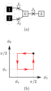
Figure 5: (a) Configuration for a rotation around $x$ axis, $U_{X}$. The computational bases is encoded over the two (solid) boxes, not in a single box. (b) An adiabatic path in the parameter space to achieve $U_{X}$ ($\phi_{3}$ is kept constant all along the path).

In the demonstrations of implementing $U_{Z}$ and $U_{CZ}$ above, we have encoded the bases $|\bar{0}\rangle$ and $|\bar{1}\rangle$ in a single Cooper-pair box for simplicity. To realize $U_{X}$, we need to encode the basis states over two Cooper-pair boxes, e.g., box $1$ and $2$ in Fig. 5 (a): $|\bar{0}\rangle\to|01\rangle_{12}$ and $|\bar{1}\rangle\to|10\rangle_{12}$. It is straightforward to generalize the above implementations of $U_{Z}$ and $U_{CZ}$ in this two-box encoding scheme. Now we turn to the remaining single-qubit gate operation $U_{X}$. The Hamiltonian is given by

$$H=-\frac{1}{2}\sum_{n=1,2,3}\left(J_{n}\,\sigma_{n}^{+}\sigma_{0}^{-}+h.c.\right)-\frac{1}{2}h\sigma_{0}^{z}\,.$$ (15)

The degenerate subspace is defined by the two eigenstates

$$|\lambda_{1}\rangle=\left(J_{2}^{*}\,|{10}\rangle_{12}-J_{1}^{*}\,|{01}\rangle_{12}\right)\otimes|00\rangle_{03}$$ (16)

(not normalized) and

$$|\lambda_{2}\rangle=\frac{J_{3}^{*}}{|J_{1}|^{2}+|J_{2}|^{2}}\left(J_{1}|{10}\rangle_{12}+J_{2}|{01}\rangle_{12}\right)\otimes|00\rangle_{03}\\ -|00\rangle_{12}\otimes|01\rangle_{03}$$ (17)

(not normalized) both with energy $-h/2$. In this case, it is required that $\gamma_{1}=\gamma_{2}=1$ but $\gamma_{3}\neq 1$ [see discussions below Eq. (8)]. As an example, we take a closed loop shown in Fig. 5 (b) (one may choose any path starting and ending at $\phi_{1}=\phi_{2}=\pi/2$, i.e., $J_{1}=J_{2}=0$) with $\phi_{3}$ fixed. The adiabatic theory of holonomies Wilczek84a ensures that from this adiabatic cycle, a state $|\psi\rangle$ initially belonging to the eigenspace undergoes a change to $|\psi^{\prime}\rangle=U|\psi\rangle$. The unitary operator $U$ is given by $U=U_{Z}^{\dagger}(\varphi^{\prime})U_{X}(\varphi)U_{Z}(\varphi^{\prime})$ with $\varphi^{\prime}=\alpha_{3}(\phi_{3})/2-\pi/4$ and

$$\varphi=2\int_{\cos\phi_{*}}^{1}\frac{dx\;\cos\phi_{*}}{(x^{2}+\cos^{2}\phi_{*})\sqrt{1+(x^{2}+\cos^{2}\phi_{*})/A_{3}^{2}(\phi_{3})}}\,.$$ (18)

Removing the first and last factors of $U_{Z}$ (if necessary) with additional phase-shift operations, one can achieve $U_{X}$.

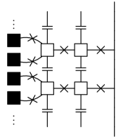
Figure 6: A computational network for universal holonomic quantum computation.

Finally, a quantum network can be constructed as in Fig. 6 to perform all the unitary operations discussed above (and hence universal quantum computation) geometrically. It is noted that the coupling capacitance $C_{c}$ is not tunable, but it suffices to have a control over each tunable junction (i.e. SQUID) and gate voltage.

IV Discussion

So far we have discussed fundamental requirements for geometric manipulations in idealized systems. In this section, we discuss several situations one may come up with when attempting an experimental realization of the present scheme.

First of all, the present scheme is based on the adiabatic theorem Messiah61b . Ideally the change in the control parameters should be infinitely slow. At a finite rate of change, there can be a transition out of the computational subspace. However, typically such a Landau-Zener-type transition occurs with an exponentially small probability $P\sim\exp(-\pi\Delta/\eta)$, where $\hbar\Delta$ is the smallest energy gap between the computational subspace and the nearby energy levels and $\eta$ is the adiabaticity parameter (i.e., $\frac{\partial}{\partial t}H(t)\sim\eta\hbar\Delta$) ZenerComment ; Berry90a ; HwangJT77a ; Dykhne61a ; Zener32a . In Josephson networks the level distance is of order of the Josephson coupling energy, $\Delta\sim E_{J}/\hbar\sim(80\,\mathrm{ps})^{-1}$. For an operation time $\tau_{\mathrm{op}}=1/\eta\gtrsim 3/\Delta$, $P\lesssim 10^{-4}$. (For comparison, in a recent experiment concerning dynamic quantum computation on Josephson qubits Nakamura99a , the switching time was no shorter than $0.25\hbar/E_{J}\sim 20\,\mathrm{ps}$.)

In the previous section, on each superconducting box we neglected higher charge states other than the two lowest. In dynamic quantum computation schemes, the existence of those higher levels may cause the quantum leakage errors, i.e., it leads to a nonzero probability of leakage out of the computational space, and more severely to renormalization of the energy levels in the computational space (which therefore reduces the gate fidelity) Fazio99b . In Josephson qubits, however, the coupling to the higher charge states are only through the Josephson tunneling of Cooper pairs, which can be easily included in our considerations [see Eqs. (4), (6), (10), and (15)]. Those higher charge states form well-separated energy levels, and do not alter the degenerate structure of the subspace in question, at least up to the order of $(E_{J}/E_{C})^{2}$ [in the dynamic scheme the quantum leakage error occurs already in the order of $(E_{J}/E_{C})^{2}$, see Ref. Fazio99b, ]. The leakage to the higher charge states out of the computational subspace can therefore be considered within the framework of Landau-Zener tunneling, which has already been discussed above. The renormalization of (degenerate) energy of the computational space is irrelevant in our geometric scheme since it does not rely on the dynamical time-evolution operator but only on the purely geometric means.

In reality there are fluctuations of the (reduced) flux $\phi$ (tuning the junctions) and the gate-induced charge $2en_{g}$ (resulting from the fluctuations of random charges in the substrate or gate voltage itself). One consequence of these fluctuations is the Landau-Zener-type transitions out of the computational subspace. A recent experiment on Josephson charge qubits Nakamura01z suggests that fluctuations of $n_{g}$ as well as $\phi$ are dominated by low frequency fluctuations. Therefore, the Landau-Zener-type transitions might be small. The fluctuations of $n_{g}$ can cause another type of errors: While the eigenspace is by construction robust against the low-frequency fluctuations of $\phi$, the random charge fluctuations lift the degeneracy of the computational subspace. The wave function of the system then acquires dynamically accumulated phase factors $\exp(-i\delta{E}\tau_{\mathrm{op}}/\hbar)$, where $\delta{E}$ is the small level spacing caused by the fluctuations of $n_{g}$. Such dynamical phases can be ignored for sufficiently small fluctuations and sufficiently short – yet long enough for adiabaticity – operation time ($1/\Delta\ll\tau_{\mathrm{op}}\ll 1/\delta{E}$).

Another common source of decoherence in Josephson charge qubits is the quasi-particle tunneling Schon90a . In particular, since the computational eigenspace is not the lowest energy states [Eq. (4) and Fig. 2 (b)], it gives rise to the relaxation out of the eigenspace to lower energy states (this effect cannot be described by the Landau-Zener-type transitions). At sufficiently low temperatures compared with the superconducting gap $\Delta_{S}$, the quasi-particle tunneling rate $\Gamma_{\mathrm{qp}}$ is exponentially small Schon90a , $\Gamma_{\mathrm{qp}}\sim\exp[-(2\Delta_{S}+E_{C})/k_{B}T]$. For example, in the experiment on Cooper-pair box Nakamura99a , $\Gamma_{\mathrm{qp}}\sim(6\,\mathrm{ns})^{-1}\sim 10^{-2}E_{J}/\hbar$ at temperature $30\,\mathrm{mK}$ even through the probe junction which was biased by a voltage $eV\sim 2\Delta_{S}+E_{C}$ (without the voltage bias $\Gamma_{\mathrm{qp}}$ should be even smaller). In such a situation, one can therefore conclude that the effect of quasi-particles is negligible.

For a brief comparison of the present scheme with the conventional Josephson charge qubit Makhlin99a ; Nakamura99a , we estimate the fidelity for a single phase-shift operation $U_{Z}$. The fidelity in this case is given by

$$\mathrm{fidelity}\simeq\sqrt{(1-P)[1-\sin^{4}(\delta\phi/2)]}\,,$$ (19)

where $P$ is the probability for Lanau-Zener-type transitions or quasiparticle tunnelings to occur and $\delta\phi$ is the error in phase shift due to the background charge fluctuations, i.e., $\delta\phi=\delta{E}\tau_{\mathrm{op}}/\hbar$ (see above). Taking $\Delta=(80\,\mathrm{ps})^{-1}$, $\tau_{\mathrm{op}}=3/\Delta$, $\Delta_{S}=5\Delta$, $k_{B}T=\Delta/10$, and $\delta{E}/\hbar=\Delta/10$ (see Ref. Nakamura99a, ), one estimates $\mathrm{fidelity}\simeq 0.998$. In the dynamic scheme the fidelity is also given by the same form as Eq. (19). The differences are that $P$ is mainly responsible for the quasiparticle tunnelings and that the phase error $\delta\phi$ comes from the finite ramping time of the gate pulse. Taking the parameters from the recent experiment Nakamura99a , we see that the fidelity takes the same value (up to three digits below decimal point).

Lastly, in ideal case some tunable junctions [e.g., $J_{1}$ in Eq. (6), see discussions below Eq. (8)] need to be turned off completely. In reality, the Josephson energies of the two parallel junctions on a SQUID loop (Fig. 1) may not be identical [i.e., $\gamma\neq 1$ in Eq. (1) and Fig. 1]. Then, a tunable junction (i.e. SQUID) cannot be turned off completely Falci00a . This makes it nontrivial to prepare an initial state which should be a product state of the “true” qubit and the ancilla qubits in a logical block [see, e.g., $|\lambda_{1}\rangle$ below Eq. (6)]. In practice, such a difficulty can be overcome by means of fast relaxation processes with the gate voltages of the ancilla qubits adjusted far off the resonance in the initial state-preparation stage. This process also allows for preparation of the “true” qubit in a definite initial state Makhlin99a .

V Conclusion

We have proposed a scheme based on geometric means to implement quantum computation on solid-state devices. The main advantage of a geometric computation scheme is its intrinsically fault-tolerant feature Preskill99a ; Ellinas01a . However, it is usually non-trivial to find a physical system whose Hamiltonian has a particular degenerate structure for geometric computation. The scheme discussed in this work provides a generic way to construct such a system from arbitrary quantum two-state systems as long as couplings satisfy certain requirements specified above. Such requirements are rather easy to fulfill on solid-state devices. A drawback of this scheme is that it requires more resources (four Cooper-pair boxes per each qubit). Considering quantum error correcting codes, however, it may not be a major disadvantage. Moreover, since the current scheme is based on adiabatic evolution, it does not require sharp pulses of flux and gate voltage. With current technology, it is still challenging to obtain a sufficiently sharp pulses of flux and gate voltages (in Ref. Nakamura99a, , the raising and falling times were of order of $\hbar/E_{J}$). Finite raising and falling times of pulses can result in a significant error in dynamic computation schemes ChoiMS01a .

- (1) Macroscopic Quantum Coherence and Quantum Computing, edited by D. V. Averin, B. Ruggiero, and P. Silvestrini (Kluwer Academic/Plenum Publishers, New York, 2001).
- (2) P. Zanardi and M. Rasetti, Phys. Lett. A 264, 94 (1999).
- (3) J. Pachos, P. Zanardi, and M. Rasetti, Phys. Rev. A 61, 010 305(R) (2000); J. Pachos and P. Zanardi, Int. J. Mod. Phys. B 15, 1257 (2001).
- (4) J. Preskill, in Introduction to Quantum Computation and Information, edited by H.-K. Lo, S. Popescu, and T. Spiller (World Scientific, Singapore, 1999), p. 154.
- (5) D. Ellinas and J. Pachos, Phys. Rev. A 64, 022 310 (2001).
- (6) F. Wilczek and A. Zee, Phys. Rev. Lett. 52, 2111 (1984).
- (7) J. A. Jones, V. Vedral, A. Ekert, and G. Castagnoli, Nature 403, 869 (2000).
- (8) G. Falci, R. Fazio, G. Massimo Palma, J. Siewert, and V. Vedral, Nature 407, 355 (2000).
- (9) J. Pachos and S. Chountasis, Phys. Rev. A 62, 052 318 (2000).
- (10) L.-M. Duan, J. I. Cirac, and P. Zoller, Science 292, 1695 (2001).
- (11) Y. Makhlin, G. Schön, and A. Shnirman, Nature 398, 305 (1999).
- (12) Y. Nakamura, Y. A. Pashkin, and J. S. Tsai, Nature 398, 786 (1999).
- (13) In this paper, we consider only Josephson charge qubits. There are literatures which discuss Josephson phase qubits; see, e.g., J. E. Mooij, T. P. Orlando, L. Levitov, L. Tian, C. H. van der Wal, and S. Lloyd, Science 285, 1036 (1999); D. Vion, A. Aassime, A. Cottet, P. Joyez, H. Pothier, C. Urbina, D. Esteve, and M. H. Devoret, Science 296, 886 (2002); F. W. Strauch, P. R. Johnson, A. J. Dragt, C. J. Lobb, J. R. Anderson, and F. C. Wellstood, quant-ph/0303002.
- (14) M. Tinkham, Introduction to Superconductivity, 2 ed. (McGraw-Hill, New York, 1996).
- (15) S. Lloyd, Phys. Rev. Lett. 75, 346 (1995).
- (16) M. V. Berry, Proc. R. Soc. London A 392, 45 (1984).
- (17) M.-S. Choi, M. Y. Choi, T. Choi, and S.-I. Lee, Phys. Rev. Lett. 81, 4240 (1998).
- (18) H. Shimada and P. Delsing, Phys. Rev. Lett. 85, 3253 (2000).
- (19) D. V. Averin, A. N. Korotkov, and Y. V. Nazarov, Phys. Rev. Lett. 66, 2818 (1991).
- (20) M. Matters, J. J. Versluys, and J. E. Mooij, Phys. Rev. Lett. 78, 2469 (1997).
- (21) A. Messiah, Quantum Mechanics (North-Holland Publishing Co., Amsterdam, 1961), Vol. 2.
- (22) Precisely, the estimation is valid for Landau-Zener tunneling between non-degerate levels. In many cases, however, this gives a good estimates also for degenerate levels. See, e.g., Yu. N. Demkov and V. N. Ostrovsky, J. Phys. B 34, 2419 (2001), and references therein.
- (23) M. V. Berry, Proc. R. Soc. London A 430, 405 (1990).
- (24) J.-T. Hwang and P. Pechukas, J. Chem. Phys. 67, 4640 (1977).
- (25) A. M. Dykhne, Zh. Eksp. Teor. Fiz. 41, 1324 (1961), [Sov. Phys.-JETP 14, 941 (1962)].
- (26) C. Zener, Proc. R. Soc. London 137, 696 (1932).
- (27) R. Fazio, G. M. Palma, and J. Siewert, Phys. Rev. Lett. 83, 5385 (1999).
- (28) G. Schön and A. D. Zaikin, Phys. Rep. 198, 237 (1990).
- (29) M.-S. Choi, R. Fazio, J. Siewert, and C. Bruder, Europhys. Lett. 53, 251 (2001).
- (30) Y. Nakamura, Yu. A. Pashkin, T. Yamamoto, and J. S. Tsai, Phys. Rev. Lett. 88, 47901 (2002).