Destabilization of dark states and optical spectroscopy in Zeeman-degenerate atomic systems

Abstract

We present a general discussion of the techniques of destabilizing dark states in laser-driven atoms with either a magnetic field or modulated laser polarization. We show that the photon scattering rate is maximized at a particular evolution rate of the dark state. We also find that the atomic resonance curve is significantly broadened when the evolution rate is far from this optimum value. These results are illustrated with detailed examples of destabilizing dark states in some commonly-trapped ions and supported by insights derived from numerical calculations and simple theoretical models.

I Introduction

Under certain conditions a laser-driven atom will optically pump into a dark state, in which the atom cannot fluoresce because the coupling to every excited state vanishes Orriols:1979 ; Arimondo:1976 . When the dark state is an angular momentum eigenstate, this phenomenon is called optical pumping. In the more general case in which the dark state is a coherent superposition of angular momentum eigenstates and the matrix elements vanish through quantum interference, it is usually called “coherent population trapping” Gray:1978 . Dark states are the basis of the STIRAP For:1998 method for adiabatic manipulation of atomic states and the VSCPT Aspect:1988 sub-recoil laser cooling scheme, and they are closely related to the quantum interference-based mechanism of lasing without inversion Harris:1989 . However, sometimes population trapping in dark states is detrimental rather than beneficial, such as when fluorescence is used to determine the state of an atom obald:1989 or when atoms are laser-cooled by scattering photons Wineland:1975 ; Hansch:1975 . Trapped ions illustrate this point very well, because their superb isolation from external perturbations can make the lifetime of coherent dark states extremely long. In such systems, laser cooling rates will be drastically reduced when the atom pumps into a dark state. One also finds that the laser cooling transition can be significantly broadened when there is significant accumulation of population in dark states, thereby reducing the cooling rate. Although some methods for restoring atomic fluorescence have been briefly discussed in the context of specific atoms, a general prescription for destabilizing dark states does not seem to exist. The aim of this paper is to provide this information, supported by insights derived from numerical calculations and simple theoretical models.

The paper is laid out as follows. In Sec. II we review the physics of dark states Arimondo:1996 ; Bruce:1990 . In Sec. III we discuss in general terms some methods of destabilizing dark states. These techniques involve either splitting the atomic energy levels (most commonly with a magnetic field Janik:1985 ; Janik:1984 ), or modulating the laser polarization Jon:1994 ; Barwood:1998 ; Berkeland:1998 . In Sec. IV we consider the application of these methods to the level systems encountered in some commonly-trapped ions. There we solve the equations of motion for the atomic density matrix to find the excited state population as a function of the various experimental parameters. We also discuss destabilizing dark states in generic two-level atoms. We conclude in Sec. V with a brief discussion of the implications of these calculations and a summary of the general prescription for destabilizing dark states.

II Dark states

We will mostly consider a two-level atom in which the total angular momenta of the lower and upper levels are $J_{i}$ and $J_{f}$ respectively, with corresponding magnetic quantum numbers $m_{i}$ and $m_{f}$. In many cases of interest the atomic levels are further split by the hyperfine interaction, which introduces the possibility of optical pumping into other lower state hyperfine levels. We will address this complication briefly in Sec. IV.3. Since we will be primarily interested in scattering photons at a high rate we consider only electric dipole transitions.

The atom is driven by a laser field

$$\textsf{{E}}(t)=\frac{1}{2}\textbf{E}(t)e^{-i\omega_{L}t}+c.c.~{},$$ (1)

where $c.c.$ denotes the complex conjugate and $\omega_{L}$ is the laser frequency. It is convenient to expand the slowly-varying amplitude $\textbf{E}(t)$ in terms of its irreducible spherical components. These are related to the Cartesian components by Weissbluth:1978 , Edmonds:1960

$$E_{\pm 1} = \mp\frac{1}{\sqrt{2}}(E_{x}\pm iE_{y})$$ (2a)

$$E_{0} = E_{z}.$$ (2b)

The advantage of this decomposition is that the components $E_{+1}$, $E_{0}$, and $E_{-1}$ (corresponding to $\sigma^{-}$, $\pi$, and $\sigma^{+}$ polarizations) drive pure $\Delta m=-1,0,\text{~{}and~{}}+1$ transitions respectively. In the the rotating wave interaction picture Bruce:1990 , the electric dipole interaction operator $-e\textbf{r}\cdot\textsf{{E}}(t)$ is then

$$-\frac{1}{2}e\textbf{r}\cdot\textbf{E}=\frac{1}{2}er\left(E_{+1}C_{-1}^{(1)}-E_{0}C_{0}^{(1)}+E_{-1}C_{+1}^{(1)}\right),$$ (3)

where $C_{q}^{(1)}\equiv\sqrt{4\pi}Y_{1q}$ are the components of the reduced spherical harmonic of rank 1. The non-zero matrix elements of this operator are given by the Wigner-Eckart theorem as

$$\left\langle J_{i},m_{i}\left|-\frac{1}{2}e\textbf{r}\cdot\textbf{E}\right|J_{f},m_{f}\right\rangle$$ (6)

$$= -\frac{1}{2}(-)^{J_{i}-m_{i}}$$

$$\times\sum_{q=-1}^{1}{(-)^{q}E_{-q}\left(\begin{array}[]{ccc}J_{i}&1&J_{f}\\ -m_{i}&q&m_{f}\\ \end{array}\right)\left\langle J_{i}\left\|er\right\|J_{f}\right\rangle}.$$

The transition Rabi frequency $\Omega_{m_{i}m_{f}}$ is defined, as usual, so that the matrix element (6) is equal to $-\frac{1}{2}\hbar\Omega_{m_{i}m_{f}}$. We will also make frequent use of the rms Rabi frequency $\Omega$ Bruce:1990 , defined by the relationship

$$\Omega^{2}=\sum_{m_{i},m_{f}}\left|\Omega_{m_{i}m_{f}}\right|^{2}$$ (7)

Now, a general superposition of lower level states

$$\left|d\right\rangle=\sum_{m_{i}}{c_{m_{i}}\left|J_{i},m_{i}\right\rangle}$$ (8)

will be dark if the electric dipole matrix element

$$\left\langle d\left|-e\textbf{r}\cdot\textbf{E}\right|f\right\rangle=0$$ (9)

vanishes for every excited state $|f\rangle$. For example, in the simple ${J_{i}=1}\leftrightarrow{J_{f}=0}~{}$system, Eqs. (8) and (9) give a single equation for the dark state

$$c_{-1}E_{+1}+c_{0}E_{0}+c_{+1}E_{-1}=0.$$ (10)

This equation has a non-trivial solution for any static laser field E, which has the important consequence that an atom driven on a ${J_{i}=1}\leftrightarrow{J_{f}=0}~{}$transition by light of constant polarization will always be pumped into a dark state. For this transition, Eq. (10) has a two-dimensional solution space spanned by the states

$$\left[\begin{array}[]{c}c_{-1}\\ c_{0}\\ c_{+1}\\ \end{array}\right]=\frac{1}{\sqrt{E_{-1}^{2}+E_{+1}^{2}}}\left[\begin{array}[]{c}-E_{-1}\\ 0\\ E_{+1}\\ \end{array}\right]$$ (11a)

and

$$\left[\begin{array}[]{c}c_{-1}\\ c_{0}\\ c_{+1}\\ \end{array}\right]=\frac{1}{\sqrt{(E_{-1}^{2}+E_{+1}^{2})(E_{-1}^{2}+E_{0}^{2}+E_{+1}^{2})}}$$ (11e)

$$\times\left[\begin{array}[]{c}-E_{0}E_{+1}\\ E_{-1}^{2}+E_{+1}^{2}\\ E_{0}E_{-1}\\ \end{array}\right],$$ (11i)

except when the laser light is $$\pi$$-polarized, in which case the space of dark states is spanned by

$${\left[\begin{array}[]{c}c_{-1}\\ c_{0}\\ c_{+1}\\ \end{array}\right]=\left[\begin{array}[]{c}1\\ 0\\ 0\\ \end{array}\right]}\textrm{~{}and~{}}{\left[\begin{array}[]{c}c_{-1}\\ c_{0}\\ c_{+1}\\ \end{array}\right]=\left[\begin{array}[]{c}0\\ 0\\ 1\\ \end{array}\right]}$$ (11j)

Table 1 summarizes the conditions under which Zeeman degenerate systems can have dark states. It shows that there is always at least one dark state if $J_{f}=J_{i}-1$, or if $J_{f}=J_{i}$ and $J_{f}$ is an integer. These are the cases which we address in this paper. The dark states for the simplest of these systems, found by solving Eq. (9), are listed in Table 2.

Table 1: Existence of dark states for arbitrary atomic systems and laser polarization in zero magnetic field.

Upper level	Lower level
$J_{f}$	Integer $J_{i}$	Half-integer $J_{i}$
$J_{i}$ + 1	No dark state	No dark state
$J_{i}$	One dark state for any polarization	One dark state for circular polarization only
$J_{i}-1$	Two dark states for any polarization	Two dark states for any polarization

Table 2: Unnormalized dark states for several atomic systems when laser light is not $\pi$-polarized. For $\pi$-polarized light, the dark states are $|J_{i},m_{i}=0\rangle$ for integer $J_{i}\leftrightarrow J_{i}$ transitions and $|J_{i},m_{i}=\pm J_{i}\rangle$ for $J_{i}\leftrightarrow J_{i}-1$ transitions

$J_{i}$	$J_{f}$	dark states(s) $\left[\begin{array}[]{c}c_{-J_{i}}\\ \vdots\\ c_{+J_{i}}\end{array}\right]$
1	0	${\left[\begin{array}[]{c}{E_{-1}}\\ {0}\\ {E_{+1}}\end{array}\right]}$ and ${\left[\begin{array}[]{c}{E_{0}E_{+1}}\\ {-\left({E_{-1}^{2}+E_{+1}^{2}}\right)}\\ {E_{0}E_{-1}}\\ \end{array}\right]}$
1	1	${\left[{{\begin{array}[]{c}{E_{-1}}\\ {-E_{0}}\\ {E_{+1}}\\ \end{array}}}\right]}$
$\frac{3}{2}$	$\frac{1}{2}$	${\left[{{\begin{array}[]{c}{\sqrt{2}E_{-1}E_{0}}\\ {-\sqrt{3}E_{-1}E_{+1}}\\ {0}\\ {E_{+1}^{2}}\\ \end{array}}}\right]}$ and ${\left[{{\begin{array}[]{c}{E_{+1}\left({3E_{-1}^{2}+E_{-1}E_{+1}^{2}-2E_{0}^{2}E_{+1}}\right)}\\ {\sqrt{6}E_{0}\left({E_{-1}^{3}+E_{+1}^{3}}\right)}\\ {-\sqrt{3}\left({E_{+1}^{4}+E_{-1}^{2}\left({2E_{0}^{2}+3E_{+1}^{2}}\right)}\right)}\\ {-\sqrt{2}E_{-1}E_{0}\left({E_{+1}\left({E_{-1}-3E_{+1}}\right)-2E_{0}^{2}}\right)}\\ \end{array}}}\right]}$
2	1	${\left[{{\begin{array}[]{c}{E_{-1}\left({E_{-1}E_{+1}-2E_{0}^{2}}\right)}\\ {\sqrt{8}E_{-1}E_{0}E_{+1}}\\ {-\sqrt{6}E_{-1}E_{+1}^{2}}\\ {0}\\ {E_{+1}^{3}}\\ \end{array}}}\right]}$ and ${\left[{{\begin{array}[]{c}{-\sqrt{2}E_{0}E_{+1}\left({2E_{0}^{2}+3E_{-1}^{3}E_{+1}+E_{-1}E_{+1}^{3}-E_{0}^{2}E_{+1}^{2}}\right)}\\ {E_{-1}E_{+1}\left({E_{-1}^{4}+6E_{-1}^{2}E_{+1}^{2}+E_{+1}^{4}}\right)-2E_{0}^{2}\left({E_{-1}^{4}+E_{+1}^{4}}\right)}\\ {-\sqrt{3}E_{0}\left({-E_{-1}^{4}E_{+1}+E_{+1}^{5}+2E_{-1}^{3}\left({2E_{+1}^{2}+E_{0}^{2}}\right)}\right)}\\ {-E_{+1}^{2}\left({E_{-1}^{4}+6E_{-1}^{2}E_{+1}^{2}+E_{+1}^{4}}\right)+4E_{-1}^{2}E_{0}^{2}E_{+1}\left({E_{-1}-2E_{+1}}\right)-4E_{-1}^{2}E_{0}^{4}}\\ {\sqrt{2}E_{-1}E_{0}\left({E_{+1}^{2}\left({E_{-1}^{2}-2E_{-1}E_{+1}+3E_{+1}^{2}}\right)+E_{0}^{2}E_{+1}\left({-3E_{-1}+4E_{+1}}\right)+2E_{0}^{4}}\right)}\\ \end{array}}}\right]}$
2	2	${\left[{{\begin{array}[]{c}{E_{-1}^{2}}\\ {-\sqrt{2}E_{-1}E_{0}}\\ {-\sqrt{\frac{2}{3}}\left({E_{-1}E_{+1}+E_{0}^{2}}\right)}\\ {-\sqrt{2}E_{0}E_{+1}}\\ {E_{+1}^{2}}\\ \end{array}}}\right]}$

III Destabilizing dark states: general principles

To decrease population accumulation in dark states by making them time-dependent, one can either shift the energies $\varepsilon_{m_{i}}$ of the states $|m_{i}\rangle$ by unequal amounts with an external field, or modulate the polarization of the laser field $\textbf{E}(t)$. The general instantaneous dark state (8) then evolves in time as

$$\left|d(t)\right\rangle=\sum_{m_{i}}{c_{m_{i}}\left(\textbf{E}(t)\right)\left|J_{i},m_{i}\right\rangle e^{-i\varepsilon_{m_{i}}t/\hbar}},$$ (12)

where we have made explicit the dependence of the dark state components $c_{m_{i}}$ on the laser field (Table 2). The application of a magnetic field is probably the simplest and most widely used method of destabilizing dark states. But there are systems (for example, trapped-ion frequency standards Alan:2001 ; Peter:1997 ) in which external fields cannot be tolerated. In these cases the laser field must be modulated instead.

We will evaluate the effectiveness of a destabilization technique by calculating the excited state population (proportional, of course, to the fluorescence rate) as a function of experimental parameters. This is done computing the evolution of the atomic density matrix $\rho$ using the Liouville equation of motion

$$\frac{\partial\rho}{\partial t}=\frac{1}{i\hbar}\left[H,\rho\right]+\frac{\partial\rho_{relax}}{\partial t},$$ (13)

where $H$ includes both the rotating wave interaction picture Hamiltonian for the coupling to the laser Bruce:1990 and the Zeeman interaction with the external magnetic field. The last term in Eq. (13) accounts for the spontaneous decay of the excited states and its effect on the ground states, including the decay of coherences between the excited states into coherences between ground states Cardimona:1982 ,

$$\frac{\partial\rho_{m_{i}m_{i}^{\prime}}}{\partial t}$$ (18)

$$= (-)^{m_{i}-m_{i}^{\prime}}(2J_{f}+1)\gamma$$

$$\times \sum\limits_{m_{f}m_{f}^{\prime}}{}{\left({\begin{array}[]{ccc}{J_{f}}&{J_{i}}&1\\ {-m_{f}}&{m_{i}}&q\\ \end{array}}\right)\left({\begin{array}[]{ccc}{J_{f}}&{J_{i}}&1\\ {-m_{f}^{\prime}}&{m_{i}^{\prime}}&q\\ \end{array}}\right)\rho_{m_{f}m_{f}^{\prime}}}$$

where $q$ has the value which causes the 3-$j$ symbols to be non-zero. Equation (13) results in a system of $4(J_{i}+J_{f}+1)^{2}$ coupled differential equations which can be solved numerically and, in some simple cases, analytically Many:1 . When the laser polarization is static, the steady state solution is easily found by solving Eq. (13) with ${\partial\rho}/{\partial t}=0$. When the laser field is modulated (with period $T$), the density matrix will, in general, evolve towards a quasi-steady-state solution in which $\rho(t)=\rho(t+T)$. In these cases we compute the excited state population by averaging the quasi-steady state solution over a modulation period.

At this point, the main result of this paper can already be summarized qualitatively. There are always three relevant time scales in the problem, with three corresponding frequencies: the excited state decay rate $\gamma$, the resonant Rabi frequency $\Omega$, and the laser polarization modulation frequency or energy level shift $\delta$. The parameter $\delta$ characterizes the evolution rate of the dark state (12) (if necessary, the exact time evolution of the dark state can be found by substituting the shifted energies or the time-dependent laser field and the appropriate dark state from Table 2 into Eq. (12)). We find from our simulations that the evolution rate which maximizes the excited state population is $\delta\sim\Omega/2$. The excited state population is never large when $\Omega$ and $\delta$ are significantly different: it is small if $\Omega$ is too large because then the strongly-driven atom is able to follow the evolving dark state adiabatically, and also if $\delta$ is too large because then the atom and the laser become detuned. We find also that the transition line shape is broadened in both of these limits ($\Omega/\delta\gg 1$ and $\Omega/\delta\ll 1$). This can be a practical concern when laser cooling an ion, because the Doppler-limited temperature of a Doppler-cooled atom is proportional to the resonance width Wayne:1982 . The ultimate temperature of the ion can therefore be substantially increased if $\delta$ is not optimum, both because the scattering rate is decreased and also because the width of the transition is increased. Fortunately, the conditions that maximize the excited state population also minimize the transition linewidth, and we find that making both $\Omega$ and $\delta$ about a fifth of the decay rate $\gamma$ leads to appreciable excited state population without significantly broadening the transition.

IV Destabilizing dark states in specific atomic systems

We now consider the application of the techniques discussed above to some commonly used atomic systems. We begin in Sec. IV.1 with the ${J_{i}=1}\leftrightarrow{J_{f}=0}~{}$system, which illustrates the basic properties of the destabilization methods in two-level systems. Then, in Sec. IV.2, we discuss the bichromatic $\Lambda$-system of ${J_{i1}=\frac{1}{2}}\leftrightarrow{J_{f}=\frac{1}{2}}\leftrightarrow{J_{i2}=\frac{3}{2}}$. This complex system illustrates several important consequences of dark states for some commonly-trapped ions. Finally, in Sec. IV.3 we generalize these results to two-level systems with higher values of the total angular momentum (the specific case of the $J=5\leftrightarrow J=5$ system has already been discussed elsewhere by one of us Boshier:2000 ).

When a magnetic field B is applied to the atom, we will choose the quantization axis to be parallel to B, and we will assume that the laser light is linearly polarized at an angle $\theta_{\text{BE}}$ to B. This choice of polarization makes the calculations somewhat simpler, and it is generally more straightforward to implement in the laboratory than solutions using circularly or elliptically polarized light. Also, if a transition has a dark state, we find that driving it with circularly or elliptically polarized light does not significantly change the optimum efficiency of the techniques discussed here. We will measure the strength of the magnetic field in terms of the Zeeman shift frequency $\delta_{B}=\mu_{B}|\textbf{B}|/\hbar$, where $\mu_{B}$ is the Bohr magneton. The detuning of the laser frequency $\omega_{L}$ from the unperturbed atomic resonance frequency $\omega_{0}$ is $\Delta=\omega_{L}-\omega_{0}$, and the total decay rate of the excited level is $\gamma$. Finally, we will usually assume that laser linewidths are negligible compared to the relevant decay rates.

IV.1 ${J_{i}=1}\leftrightarrow{J_{f}=0}~{}$

The simple ${{}^{2}S_{1}}\leftrightarrow{{}^{2}P_{0}}$, ${J_{i}=1}\leftrightarrow{J_{f}=0}~{}$transition is well-suited to discussing in detail the main methods of destabilizing dark states. Also, the closely-related nuclear spin $I=\frac{1}{2}$, $F_{i}=1\leftrightarrow F_{f}=0$ transition is used in laser cooling and fluorescence detection in both ${}^{199}\text{Hg}^{+}$ Berkeland:1998 and ${}^{171}\text{Yb}^{+}$ Roberts:1999 ; Enders:1993 ; Fisk:1997 ; Tamm:1995 ($F$ denotes as usual the total angular momentum in atoms with non-zero nuclear spin). Decays to the $F_{i}=0$ state in these systems are infrequent, occurring only through off-resonance excitation of the $F_{f}=1$ level. The atom can be pumped out of the $F_{i}=0$ state by a microwave field driving the ${|F_{i}=0,m_{i}=0\rangle}\leftrightarrow{|F_{i}=1,m_{i}=0\rangle}$ transition Roberts:1999 ; Enders:1993 , or by a laser field driving a ${|F_{i}=0,m_{i}=0\rangle}\leftrightarrow{|F_{f}=1\rangle}$ transition Berkeland:1998 . As long as this pumping mostly keeps the population within the $F_{i}=1$ and $F_{f}=0$ levels, the results for these real systems are nearly identical to those for the $I=0$, ${{}^{2}S_{1}}\leftrightarrow{{}^{2}P_{0}}$ transition we discuss here.

The next two sections discuss destabilizing dark states in this system, firstly with a magnetic field, and then with polarization modulation.

IV.1.1 Destabilization with a magnetic field

The steady-state solution of Eq. (13) for the ${J_{i}=1}\leftrightarrow{J_{f}=0}~{}$system in a magnetic field can be found analytically. The resulting expression for the excited state population is

$$P_{f}=\frac{3}{4}\frac{\Omega^{2}\cos^{2}\theta_{\text{BE}}\sin^{2}\theta_{\text{BE}}}{1+3\cos^{2}\theta_{\text{BE}}}\frac{1}{(\gamma^{\prime}/2)^{2}+\Delta^{2}},$$ (20)

where

$$\left(\frac{\gamma^{\prime}}{2}\right)^{2}=\left(\frac{\gamma}{2}\right)^{2}+\Omega^{2}\cos^{2}\theta_{\text{BE}}\frac{1-3\cos^{2}\theta_{\text{BE}}}{1+3\cos^{2}\theta_{\text{BE}}}$$

$$+\frac{\cos^{2}\theta_{\text{BE}}}{1+3\cos^{2}\theta_{\text{BE}}}\left(\frac{\Omega^{4}}{16\delta_{B}^{2}}+16\delta_{B}^{2}\right),$$ (21)

and $\Omega$ is the rms Rabi frequency defined in Eq. (7). In our normalized units, the Zeeman shifts of the $m_{i}=\pm 1$ ground states are $\pm 2\delta_{B}$ respectively, so the dark state evolution rate is $\delta=2\delta_{B}$.

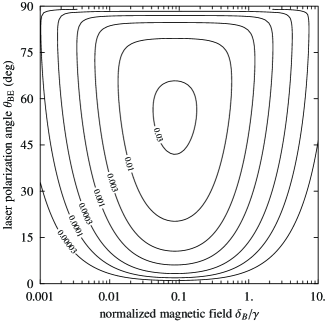
Figure 1: Excited state population $P_{f}$ in the ${J_{i}=1}\leftrightarrow{J_{f}=0}~{}$transition as a function of normalized magnetic field $\delta_{B}/\gamma$ and laser polarization angle $\theta_{\text{BE}}$. The rms Rabi frequency $\Omega=\frac{\sqrt{3}}{5}\gamma$ and the laser detuning $\Delta=0$.

Figure 1 is a graph of the excited state population $P_{f}$ as a function of magnetic field strength and polarization angle for a convenient value of Rabi frequency. It shows that there is both an optimum magnetic field strength and an optimum polarization angle for the laser field. $P_{f}$ vanishes when $\theta_{\text{BE}}=0^{\circ}$ or $90^{\circ}$ because the atom then optically pumps into the $m_{i}=\pm 1$ states or the $m_{i}=0$ state respectively. One finds from Eq. (20) that the excited state population is maximized for a given Rabi frequency by choosing the magnetic field strength so that $\delta_{B}=\Omega/4$ and the laser polarization angle so that $\theta_{\text{BE}}=\arccos\frac{1}{\sqrt{3}}$ (the angle which makes the three transition Rabi frequencies equal). Figure 2(a) shows $P_{f}$ as a function of Rabi frequency and magnetic field for this optimum angle. The excited state population is, as expected, small in both the low intensity regime $\Omega<\gamma$ and in the large-detuning regime $\delta_{B}>\gamma$. However, it is also small even at high intensity ($\Omega>\gamma$) if $\delta_{B}\ll\Omega$. Our simulations show that this occurs because under these conditions the atom adiabatically follows the evolving instantaneous dark state. On the other hand, near the optimum condition $\delta_{B}=\Omega/4$ the dark state evolves quickly enough that the atom never entirely pumps into it, and so the excited state population can be substantial.

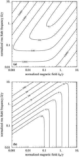
Figure 2: (a) Excited state population, and (b) resonance width (in units of $\gamma$) as a function of normalized magnetic field and normalized rms Rabi frequency for the ${J_{i}=1}\leftrightarrow{J_{f}=0}~{}$transition with $\theta_{\text{BE}}=\arccos\frac{1}{\sqrt{3}}$ and $\Delta=0$.

In many applications the linewidth of the transition is also an important quantity. Fig. 2(b) shows the dependence of the resonance width $\gamma^{\prime}$ on the Rabi frequency and the magnetic field. We see that the linewidth is large when $\delta_{B}>\gamma$ because of Zeeman broadening, when $\Omega>\gamma$ because of ordinary power broadening (the second term in Eq. (IV.1.1)), and also when $\delta_{B}\ll\Omega$, a less obvious regime which will be discussed below. Figures 2(a) and 2(b) illustrate the useful result (easily obtained from Eqs. (20) and (IV.1.1)) that maximizing the excited state population for a particular Rabi frequency also minimizes the resonance line width. These plots show that the choice $\Omega\sim\gamma/3$ gives substantial excited state population without significantly increasing the linewidth. If the linewidth is not important, then the laser intensity can be chosen to saturate the transition ($\Omega\gg\gamma$) and the magnetic field strength then adjusted so that $\delta_{B}=\Omega/4$.

The broadening of the resonance when $\delta_{B}\ll\Omega$ is apparent in Eq. (IV.1.1), which contains the terms

$$\frac{\cos^{2}\theta_{\text{BE}}}{1+3\cos^{2}\theta_{\text{BE}}}\left(\frac{\Omega^{4}}{16\delta_{B}^{2}}+16\delta_{B}^{2}\right).$$ (22)

The term proportional to $\delta_{B}^{2}$ is simple Zeeman broadening, but the term proportional to $1/\delta_{B}^{2}$ does not have an obvious physical interpretation. We find that such a broadening term is present whenever the atom contains a $\Lambda$-system, regardless of the method of destabilizing the dark state. To understand this behavior in simple physical terms, consider Fig. 3(a), which shows a generic $\Lambda$-system in which the laser field drives only one arm of the system, with Rabi frequency $\Omega$. $|i\rangle$ and $|d\rangle$ represent light and dark ground states respectively. The excited state decays to the two ground states with branching ratio $(1-\alpha):\alpha$. All of the systems discussed in this paper can be described similarly (although with higher multiplicity of states) after a change in basis states. For example, in the ${J_{i}=1}\leftrightarrow{J_{f}=0}~{}$transition driven by $\pi$-polarized light, $|d\rangle$ corresponds to either the $m_{i}=1$ or $m_{i}=-1$ state, $|i\rangle$ corresponds to the $m_{i}=0$ ground state and $|f\rangle$ corresponds to the excited state. For simplicity, in this generic case the coupling between the light and dark ground states is represented by an incoherent rate $R$, rather than the coherent magnetic field. When the steady-state density matrix equations are solved for this system, the population of the excited state $|f\rangle$ is found to be

$$P_{f}=\frac{\frac{1}{8}\Omega_{\text{if}}^{2}}{\frac{1}{4}\gamma^{2}+\frac{3}{8}\Omega_{\text{if}}^{2}+\frac{1}{8}\alpha\gamma\Omega_{\text{if}}^{2}/R+\Delta_{\text{if}}^{2}},$$ (23)

where $\Delta_{\text{if}}$ is the detuning of the laser frequency from resonance with the atomic transition. The term $\frac{1}{8}\alpha\gamma\Omega_{\text{if}}^{2}/R$ is analogous to the broadening term $\Omega^{4}/16\delta_{B}^{2}$ in Eq. (IV.1.1). In both cases the linewidth becomes large as the dark ground state is coupled less strongly to the light ground state.

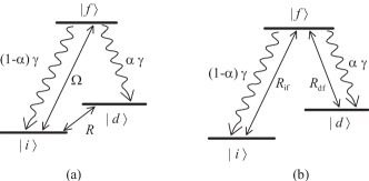
Figure 3: Generic three-level $\Lambda$-systems with (a) incoherent coupling between ground states, and (b) laser coupling of both transitions.

For trapped ions this behavior has a simple physical explanation in terms of quantum jumps. Suppose that $\alpha\ll 1$, so most of the decays are to state $|i\rangle$, and also that the pump rate $R$ out of the dark state $|d\rangle$ is very small. Then, as long as the atom is not in state $|d\rangle$, it behaves like a two-level atom and we can use the well-known results for this system. It follows that, on average, an atom initially in state $|i\rangle$ will for a time $\Delta t=\frac{1-\alpha}{\alpha}(\frac{1}{4}\gamma^{2}+\Delta_{\text{if}}^{2})/\frac{1}{2}\Omega_{\text{if}}^{2}\gamma$ scatter $(1-\alpha)/\alpha$ photons before decaying into state $|d\rangle$. The atom will then not fluoresce for an average time $1/R$, so that on average the number of fluorescent photons emitted per unit time is

$$\bar{n} = \frac{1-\alpha}{\alpha}\left(\frac{1}{R}+\Delta t\right)^{-1}$$ (24)

$$\approx \frac{1}{\alpha}\left(\frac{1}{R}+\frac{1}{\alpha}\frac{\frac{1}{4}\gamma^{2}+\Delta_{\text{if}}^{2}}{\frac{1}{2}\Omega_{\text{if}}^{2}\gamma}\right)^{-1},$$

which agrees with the average photon emission rate $\gamma P_{f}\sim R/\alpha$ obtained from Eq. (23) in the limit of small $R$. Now the source of the broadening can be seen: if $R\ll\alpha\Omega_{\text{if}}^{2}/\gamma$ and $\Delta_{\text{if}}\lesssim\gamma$, then the time during which the atom scatters photons is very short compared to the time that it spends not fluorescing at all. The average rate of photon scattering is therefore very small and does not change much with detuning until $\Delta_{\text{if}}$ becomes much larger than $\gamma$, because then the time it takes to pump into the dark state is no longer less than the time the atom spends in the dark state. When only the average photon scattering rate is measured, the line shape as a function of laser frequency is therefore very broad. We will also consider below in Sec. IV.2.1 an explanation of the broad line shape at low incoherent pump rates in terms of rate equations Janik:1985 .

IV.1.2 Destabilization with polarization modulation

We turn now to the second category of techniques for destabilizing dark states, modulating the polarization state of the laser field. In order to destabilize dark states in a ${J_{i}=1}\leftrightarrow{J_{f}=0}~{}$system in zero magnetic field, the three spherical components of the field $E_{-1}$, $E_{0}$, and $E_{+1}$ must be non-zero and they must have linearly-independent time dependences because otherwise Eq. (10) will have a nontrivial solution. Physically this is because only one excited state is coupled to three ground states, forming two conjoined $\Lambda$-systems that must be independently destabilized. Imposing different time dependences on all three polarization components requires two non-collinear laser beams Berkeland:1998 . This makes the ${J_{i}=1}\leftrightarrow{J_{f}=0}~{}$system experimentally more complicated than every other two-level system, since Table 2 shows that their dark states can still be destabilized if one polarization component is zero and the other two have different time dependences, which requires but a single laser beam.

One obvious way of producing a suitable polarization modulation is giving the three polarization components different frequencies. This can be done, for example, by passing three linearly polarized beams through separate acousto-optic modulators (AOM’s), followed by appropriately oriented waveplates. If right- and left-handed circularly polarized light are separately shifted and copropagate along the quantization axis, while a second beam is polarized along the quantization axis, the resulting field can be written as

$$\left(\begin{array}[]{c}E_{-1}\\ E_{0}\\ E_{+1}\\ \end{array}\right)=\left(\begin{array}[]{c}E_{\sigma^{+}}e^{-i\delta_{\text{AOM-}}t}\\ 0\\ E_{\sigma^{-}}e^{-i\delta_{\text{AOM+}}t}\\ \end{array}\right)+\left(\begin{array}[]{c}0\\ E_{\pi}\\ 0\\ \end{array}\right),$$ (25)

where $\delta_{\text{AOM+}}$ and $\delta_{\text{AOM-}}$ are the relative frequency shifts due to the AOM’s, and $E_{\sigma^{+}}$, $E_{\sigma^{-}}$, and $E_{\pi}$ are the amplitudes of the three laser fields. The symmetrical conditions $\delta_{\text{AOM+}}=-\delta_{\text{AOM-}}$ and $E_{\sigma^{+}}=E_{\sigma^{-}}$ are most efficient at destabilizing dark states. In this case, the analytical solution to the density matrix equation of motion (13) is identical to that obtained when a magnetic field with $2\delta_{B}=\delta_{\text{AOM+}}$ is applied at an angle $\theta_{\text{BE}}=\arctan(\sqrt{2}E_{\pi}/E_{\sigma^{+}})$, and so the discussion accompanying Figs. 1 and 2 applies here also. The optimum parameters are therefore $|E_{+1}|=|E_{0}|=|E_{-1}|$ and $\delta_{\text{AOM+}}=-\delta_{\text{AOM-}}=\Omega/2$ and $\Omega\sim\gamma/3$. Experimentally, this is perhaps the simplest technique to destabilize dark states in this system, because AOM’s are simple, inexpensive devices.

An alternative technique for continuously altering the polarization state of the field is modulating, with different phases, the amplitudes of the polarization components of the field. In atomic beam experiments, this can be done by sending the atoms through two or more laser-atom interaction regions of different laser polarization Jon:1994 . With trapped ions, it has been demonstrated in several systems by smoothly varying the intensity ratios or relative phases of the polarization components of the light driving the stationary atoms Barwood:1998 ; Berkeland:1998 . For example Berkeland:1998 , overlapping at right angles a $\pi$-polarized laser beam with a second beam that has passed through a photo-elastic modulator (PEM) in which the fast axis is compressed while the slow axis is expanded produces the field

$$\left(\begin{array}[]{c}E_{-1}\\ E_{0}\\ E_{+1}\\ \end{array}\right)=\frac{E_{PEM}}{\sqrt{2}}\left(\begin{array}[]{c}e^{+i\varphi(t)}+ie^{-i\varphi(t)}\\ 0\\ e^{+i\varphi(t)}-ie^{-i\varphi(t)}\\ \end{array}\right)+\left(\begin{array}[]{c}0\\ E_{\pi}\\ 0\\ \end{array}\right)$$ (26)

where

$$\varphi(t)=\frac{1}{2}\Phi\left[{1-\cos\left({\delta_{PEM}t}\right)}\right],$$ (27)

$\Phi$ is the phase modulation amplitude, and $\delta_{\text{PEM}}$ is the modulation rate of the PEM indices of refraction. As above, we have defined the quantization axis to be parallel to the propagation direction of the modulated beam. If $\Phi\geq\pi$, then the polarization of the modulated beam continuously cycles between linear and right- or left-hand circular polarizations. When $\Phi>\pi$, Fourier analysis of the modulated field reveals a flat spectrum of harmonics of $\delta_{\text{PEM}}$ up to a maximum harmonic number of $\sim 2\Phi/\pi$, so that the effective dark state evolution rate in this high modulation index regime is $\delta\sim\Phi\delta_{\text{PEM}}$.

In this case the system never reaches a steady state. This can be seen in Fig. 4, which shows the numerically calculated populations of each level of the ${J_{i}=1}\leftrightarrow{J_{f}=0}~{}$system as a function of time when the field is modulated as in Eqs. (26) and (27). The field has been applied for a time of about $1000/\gamma$, sufficient in this case to reach the quasi-steady state in which the atomic state evolution is periodic. The settling time depends on the initial state of the atom, on the laser intensity, and on the modulation rate. The time evolution of the state populations seen in Figure 4 displays oscillations at the harmonics of $\delta_{\text{PEM}}$ imposed on the field by the modulation.

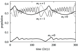
Figure 4: Populations of individual states in the ${J_{i}=1}\leftrightarrow{J_{f}=0}~{}$transition when the laser field is modulated according to Eq. (26) and the quasi-steady state has been reached. The laser detuning $\Delta=0$, phase modulation amplitude $\Phi=10\pi$, modulation frequency $\delta_{\text{PEM}}=\gamma/50$, and Rabi frequencies $\Omega_{-1,0}=\Omega_{0,0}=-\Omega_{+1,0}=\gamma/5$, so that the rms Rabi frequency $\Omega=\frac{\sqrt{3}}{5}\gamma$, as in Fig.  1.

Figure 5 shows the numerically calculated population $P_{f}$ of the excited state (averaged over time $2\pi/\delta_{\text{PEM}}$ in the quasi-steady state regime) as a function of $\delta_{\text{PEM}}/\gamma$ and the phase modulation amplitude $\Phi$. The Rabi frequencies and detunings are the same as for Fig. 1, in which the dark states were destabilized with a magnetic field. A comparison of the two graphs shows that the two techniques can be similarly efficient at destabilizing dark states. Figure 5 shows that the optimum modulation frequency is $\delta_{\text{PEM}}\sim 0.1\gamma$ for small modulation amplitudes $\Phi\lesssim\pi$, moving to lower values as $\Phi$ increases above $\pi$ and the amplitude of the sidebands increases. The excited state population is small when $\Phi\delta_{\text{PEM}}\ll\Omega$, because the atom then adiabatically follows the slowly evolving dark state. It is also small when $\Phi\delta_{\text{PEM}}\gg\gamma$ because then much of the power of the modulated field is at frequencies that are far from resonance.

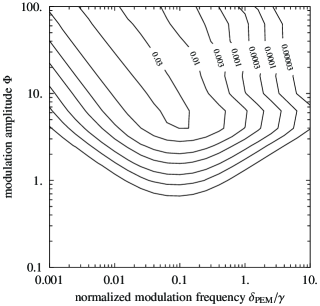
Figure 5: Excited state population $P_{f}$ in the ${J_{i}=1}\leftrightarrow{J_{f}=0}~{}$transition as a function of normalized modulation frequency $\delta_{\text{PEM}}/\gamma$ and modulation amplitude $\Phi$ for the field given by Eqs. (26) and (27). Laser intensity and detuning as for Fig. 4.

In many experimental situations it may not be possible to propagate the modulated and static linearly-polarized beams at right angles Berkeland:1998 . We have therefore repeated the calculation of Fig. 5 with the unmodulated beam polarized at angle $\arccos\frac{1}{\sqrt{3}}\sim 63^{\circ}$ to the propagation direction of the modulated beam. The time evolution of the three polarization components of the field is no longer completely orthogonal, and so the excited state population is reduced for all modulation frequencies, in this case by about a factor of three. However, the modulation frequency at which the excited state population is maximized does not change appreciably, nor does the frequency bandwidth of the atomic response to the modulation.

In correspondence with the magnetic field case discussed in the previous section, we find from our simulations that the linewidth is large when the laser intensity is high ($\Omega>\gamma$), when the modulation significantly broadens the laser frequency spectrum ($\Phi\delta_{\text{PEM}}>\gamma$) and when the evolution rate of the dark state is low ($\Phi\delta_{\text{PEM}}\ll\Omega$).

Finally, we remark that although this second polarization modulation scheme may not be the best approach for the ${J_{i}=1}\leftrightarrow{J_{f}=0}~{}$system because it needs a relatively expensive PEM, a variation of it is probably the most appealing method for destabilizing dark states in every other two-level system in zero magnetic field. In these systems, it is sufficient to use a field having only two polarization components with different time dependences. This can be accomplished very simply by passing a single beam through an electro-optic modulator (EOM), as we will discuss in the next section.

IV.2 ${{}^{2}S_{1/2}}\leftrightarrow{{}^{2}P_{1/2}}\leftrightarrow{{}^{2}D_{3/2}}~{}$

In this section we consider the ${{}^{2}S_{1/2}}\leftrightarrow{{}^{2}P_{1/2}}\leftrightarrow{{}^{2}D_{3/2}}~{}$$\Lambda$-system, which occurs in ${}^{40}\text{Ca}^{+}$ Knoop:1999 ; Urabe:1998 ; Nagerl:1999 ; Hughes:1998 ; Block:1999 , ${}^{88}\text{Sr}^{+}$ Barwood:1998 ; Bernard:1999 ; Berkeland:1 , and ${}^{138}\text{Ba}^{+}$DeVoe:1996 ; Raab:1998 ; Nagourney:1997 ; Huesmann:1999 ions. Figure 6 shows a partial energy level diagram of these atoms. The ${}^{2}P_{1/2}$ states decay to both the ${}^{2}S_{1/2}$ and the metastable ${}^{2}D_{3/2}$ levels with a branching ratio that favors the ${{}^{2}P_{1/2}}\to{{}^{2}S_{1/2}}$ decay (1:12 for Ca⁺, 1:13 for Sr⁺ and 1:2.7 for Ba⁺). Because driving the ${{}^{2}S_{1/2}}\leftrightarrow{{}^{2}P_{1/2}}~{}$laser cooling transition optically pumps the atom into the metastable ${}^{2}D_{3/2}$ level, a second ”repumping” laser is tuned near resonance with the ${{}^{2}D_{3/2}}\leftrightarrow{{}^{2}P_{1/2}}~{}$transition to pump the ion out of the ${}^{2}D_{3/2}$ states. For simplicity we assume that the ${}^{2}D_{3/2}$ state is stable, which is reasonable because the lifetime of this state is far greater than any other time scale of the system. The rms Rabi frequencies and detunings of the cooling and repumping lasers are denoted by $\Omega_{\text{SP}}$, $\Delta_{\text{SP}}$, $\Omega_{\text{DP}}$, and $\Delta_{\text{DP}}$ respectively.

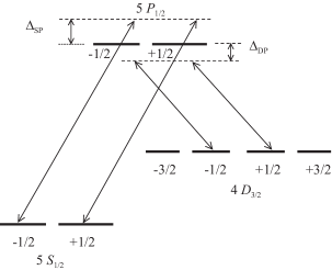
Figure 6: Partial level diagram of ${}^{88}\text{Sr}^{+}$ showing transitions driven by $\pi$-polarized laser light. This level diagram also applies to ${}^{40}\text{Ca}^{+}$ and ${}^{138}\text{Ba}^{+}$ after respectively decrementing and incrementing the principal quantum numbers by one.

Although the $J_{i}=\frac{1}{2}\leftrightarrow J_{f}=\frac{1}{2}$ cooling transition does not have a dark state, the $J_{i}=\frac{3}{2}\leftrightarrow J_{f}=\frac{1}{2}$ repumping transition does (Table 2). In the following sections we discuss methods for destabilizing this dark state. As above, we consider first destabilizion with a magnetic field, followed by a discussion of the polarization modulation technique. We will also show how coherent population trapping in dark states affects the lineshape of the cooling transition.

Convenient analytic solutions of the equation of motion for the density matrix in this complex system are not possible, and so all results presented for the ${{}^{2}S_{1/2}}\leftrightarrow{{}^{2}P_{1/2}}\leftrightarrow{{}^{2}D_{3/2}}~{}$system are based on numerical solutions.

IV.2.1 Destabilization with a magnetic field

When a magnetic field is applied to destabilize dark states in this eight-state system, the transition lineshapes develop rich structure. This can be seen in Fig. 7, which shows the cooling transition lineshape for different values of magnetic field strength, laser polarization angle, and repumping laser intensity. The structure seen around $\Delta_{\text{SP}}=+\gamma/2$ in each graph in the figure is due to coherent population trapping in superpositions of ${}^{2}S_{1/2}$ and ${}^{2}D_{3/2}$ states. These dark resonances have already been studied in several experiments with trapped ions Janik:1985 ; Siemers:1992 .

Figure 7 shows that the cooling transition lineshape is sensitive to the magnetic field, to the polarization angle, and to the intensity of the repumping laser. In cases where the evolution rate of the dark state is low, either because the the magnetic field is small (curve $E$) or the polarization angle is small (curve $D$), the resonance is broadened, for the reasons discussed above in Sec. IV.1.1. If the repumping laser intensity is high (curve $C$), then the dark resonances are power-broadened and the ${{}^{2}S_{1/2}}\leftrightarrow{{}^{2}P_{1/2}}~{}$transition displays a substantial ac Stark shift. On the other hand, when the repumping laser intensity is low (curve $B$), the resonance is again broadened.

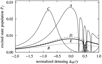
Figure 7: Population of the ${}^{2}P_{1/2}$ level of the ${}^{88}\text{Sr}^{+}$ ${{}^{2}S_{1/2}}\leftrightarrow{{}^{2}P_{1/2}}\leftrightarrow{{}^{2}D_{3/2}}~{}$system in a magnetic field as a function of normalized laser detuning $\Delta_{\text{SP}}/\gamma$. Both lasers are linearly polarized at angle $\theta_{\text{BE}}$ to the magnetic field direction, $\Omega_{\text{SP}}=\frac{\sqrt{2}}{5}\gamma$, and $\Delta_{\text{DP}}=+\gamma/2$. Curve A, and all other curves unless noted otherwise: $\theta_{\text{BE}}=90^{\circ}$, $\Omega_{\text{DP}}=\frac{\sqrt{2}}{5}\gamma$, $\delta_{B}=0.1\gamma$. Curve B: $\Omega_{\text{DP}}=\frac{\sqrt{2}}{20}\gamma$. Curve C: $\Omega_{\text{DP}}=2\sqrt{2}\gamma$. Curve D: $\theta_{\text{BE}}=10^{\circ}$. Curve E: $\delta_{B}=0.003\gamma$.

The broadening seen in curve $B$ is closely related to the broadening already encountered Sec. IV.1.1 in the regime where the dark state evolves too slowly. Its origin can be understood here most simply in terms of rate equations Janik:1985 . Figure 3(b) shows a simplified version of the system, in which two lasers drive a simple $\Lambda$-system in which the excited state $|f\rangle$ decays to the ground states $|i\rangle$ and $|d\rangle$ with branching ratio $(1-\alpha):\alpha$. The $|i\rangle\leftrightarrow|f\rangle$ transition has excitation rate $R_{\text{if}}$ and the $|d\rangle\leftrightarrow|f\rangle$ transition has rate $R_{\text{df}}$. The steady-state rate equations for this system are easily solved to give the following expression for the excited state population $P_{f}$:

$$\frac{1}{P_{f}}=3+\frac{(1-\alpha)\gamma}{R_{\text{if}}}+\frac{\alpha\gamma}{R_{\text{df}}}.$$ (28)

When the rate on the $|d\rangle\leftrightarrow|f\rangle$ transition is low, the last term in this equation dominates, so that the excited state population is insensitive to changes in the rate of the $|i\rangle\leftrightarrow|f\rangle$ transition, which in turn means that this transition is broadened. Physically, the insensitivity arises because under these conditions most of the population in the system is in state $|d\rangle$. Increasing the rate on the $|i\rangle\leftrightarrow|f\rangle$ transition then has only a very small effect on the excited state population because almost all of the population removed from state $|i\rangle$ ends up in state $|d\rangle$. There is an obvious connection here to the picture for the broadening given above in terms of quantum jumps. It follows from Eq. (28) that to avoid broadening the cooling transition, the transition rates must be such that $\alpha(1-\alpha)R_{d}>R_{i}$. In terms of the Rabi frequencies for the ${{}^{2}S_{1/2}}\leftrightarrow{{}^{2}P_{1/2}}\leftrightarrow{{}^{2}D_{3/2}}~{}$system, this condition becomes $\Omega_{\text{DP}}^{2}>\alpha\Omega_{\text{SP}}^{2}$ in the limit $\alpha\ll 1$. Another constraint on the intensities arises from the need to avoid excessive power-broadening of the dark resonances by the repumping laser, which translates into the restriction $\Omega_{\text{DP}}<\gamma/2$.

While the structure seen in Fig. 7 makes it difficult to produce meaningful graphs of the linewidth (as in Fig. 2(b)), it is still straightforward to plot the excited state population as a function of the polarization angle $\theta_{\text{BE}}$ and magnetic field strength (Fig. 8). The laser frequencies and intensities used here have been chosen to keep the dark resonances on the blue side of the laser cooling transition and to avoid power broadening. The graph is similar to the ${J_{i}=1}\leftrightarrow{J_{f}=0}~{}$case (Fig. 1), with two important differences. First, the peak is broader in both angle and in magnetic field strength. The reduced sensitivity to the magnetic field arises because this system does not pump into dark states as quickly as the ${J_{i}=1}\leftrightarrow{J_{f}=0}~{}$system, since most excited state decays are to the ${}^{2}S_{1/2}$ states and the repumping laser is detuned from resonance. It follows that the system can tolerate slower dark state evolution rates without adversely affecting the excited state population. The second difference is the set of narrow vertical dips, which are due to coherent population trapping in dark states. These dips can be seen more clearly in the thin curve in Figure 9, which shows the excited state population as a function of the magnetic field for the same conditions as those of Fig. 8 and with $\theta_{\text{BE}}=90^{\circ}$ (a convenient choice). The excited state population vanishes for two magnetic fields. First, when $\delta_{B}=\frac{5}{22}\gamma\approx 0.23\gamma$ the $|^{2}S_{1/2},m_{i}=+1/2\rangle$ and $|^{2}D_{3/2}$,$m_{i}=-3/2\rangle$ states are Zeeman shifted into Raman resonance, which forms a stable dark superposition of these two states. The same is true at $\delta_{B}=\frac{5}{6}\gamma\approx 0.83\gamma$, where the dark state is composed of the $|^{2}S_{1/2},m_{i}=+1/2\rangle$ and $|^{2}D_{3/2},m_{i}=+1/2\rangle$ states. We note that for the realistic Rabi frequencies used here, the optimum field strength, corresponding to $\delta_{B}\sim 0.05\gamma$, is well removed from the dark resonances.

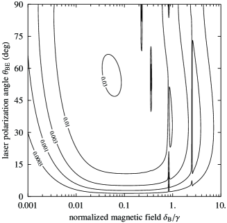
Figure 8: Population of the ${}^{2}P_{1/2}$ level of the ${}^{88}\text{Sr}^{+}$ ${{}^{2}S_{1/2}}\leftrightarrow{{}^{2}P_{1/2}}\leftrightarrow{{}^{2}D_{3/2}}~{}$system as a function of magnetic field strength and of the angle between the magnetic field and the polarization vectors of the two laser fields. The rms Rabi frequencies are $\Omega_{\text{SP}}=\Omega_{\text{DP}}=\frac{\sqrt{2}}{5}\gamma$, and the detunings are $\Delta_{\text{DP}}=+\gamma/2$ and $\Delta_{\text{SP}}=0$. The narrow vertical features are dips due to dark resonances (see also the thin curve in Fig. 9.)

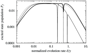
Figure 9: Excited state population as a function of dark state evolution rate $\delta$ for the ${}^{88}\text{Sr}^{+}$ ${{}^{2}S_{1/2}}\leftrightarrow{{}^{2}P_{1/2}}\leftrightarrow{{}^{2}D_{3/2}}~{}$system. Thin curve: magnetic field applied at $\theta_{\text{BE}}=90^{\circ}$, and $\delta=\delta_{B}$. Thick curve: EOM polarization modulation as in Eqs. (29) and (30) with $\Phi=\pi$, and $\delta=\delta_{\text{EOM}}$. Dashed curve: AOM polarization modulation as in Eq. (31) with $\delta_{\text{AOM+}}=-\delta_{\text{AOM-}}$, and $\delta=\delta_{\text{AOM+}}$. Laser intensities and detunings are as for Fig. 8

We conclude this section with a discussion of the optimum parameter values for destabilizing dark states with a magnetic field without excessively broadening the transition. The intensity of the cooling laser should be set to drive the cooling transition as hard as possible without power broadening it, which will be the case if $\Omega_{\text{SP}}\sim\gamma/3$. Setting the repumping laser intensity so that $\Omega_{\text{DP}}\sim\gamma/3$, will make the repumping efficient without excessively power-broadening the overall transition or the dark resonances. Since the branching ratio $\alpha\ll 1$, this choice also avoids excess broadening of the cooling transition from the mechanism discussed after Eq. (28). The detuning of the repumping laser used in Fig. 7, $\Delta_{\text{DP}}=+\gamma/2$, was chosen because it ensures that the laser still drives the repumping transition efficiently while keeping the dark resonances far from the red side of the cooling transition, where the cooling laser is tuned during Doppler cooling. The magnetic field strength should be chosen so that $0.01\gamma<\delta_{B}<0.1\gamma$ (the upper limit is less than the value of $~{}\gamma$ implied by Fig. 8 because we also wish to confine the dark resonances to a region of width $<\gamma$ to keep them all on the red side of the resonance.) Finally, although we have performed the calculations for light which is linearly polarized perpendicular to the magnetic field, Fig. 8 shows that any polarization angle greater than $15^{\circ}$ works well. In fact, our simulations show that the resonance curve is not changed significantly even if the laser polarizations are perpendicular to each other or if the repumping laser is circularly polarized.

IV.2.2 Destabilization with polarization modulation

We now consider destabilizing dark states in the ${}^{2}D_{3/2}$ level by modulating the repumping laser polarization. In this system, as in every other except the ${J_{i}=1}\leftrightarrow{J_{f}=0}~{}$system, it is sufficient to use a field having only two polarization components with different time dependences. Perhaps the simplest method of achieving this is to pass a single laser beam through an electro-optic modulator (EOM) acting as a variable waveplate to produce the field

$$\left(\begin{array}[]{c}E_{-1}\\ E_{0}\\ E_{+1}\\ \end{array}\right)=\frac{E_{EOM}}{\sqrt{2}}\left(\begin{array}[]{c}1+ie^{-i\varphi(t)}\\ 0\\ 1-ie^{-i\varphi(t)}\\ \end{array}\right),$$ (29)

where we have again defined the quantization axis to be parallel to the propagation direction of the beam. The retardation $\varphi(t)$ is similar to that of Eq. (27),

$$\varphi(t)=\frac{1}{2}\Phi\left[1-\cos(\delta_{EOM}t)\right],$$ (30)

with $\delta_{\text{EOM}}$ being the EOM drive frequency. The thick curve in Figure 9 shows the time-averaged excited state population when the polarization of the repumping laser is modulated in this way. We see that the excited state population is reduced for certain values of $\delta_{\text{EOM}}$. This is because the Fourier transform of the field of Eq. (29), like that of Eq. (26), contains harmonics of $\delta_{\text{EOM}}$ up to harmonic number $\sim 2\pi/\Phi$ when the modulation index exceeds one (so that the effective dark state evolution rate in this high modulation index regime is $\delta\sim\Phi\delta_{\text{EOM}}$). The excited state population will be reduced when one of these sidebands connects the ${}^{2}D_{3/2}$ and ${}^{2}S_{1/2}$ states in Raman resonance. In this case, where the modulation index is $\sim 1$, two such dips are visible. The excited state population does not vanish completely in these dips because the other frequency components present in the field still act to destabilize the dark state.

Another easily-realized modulation scheme gives the $\sigma^{+}$ and $\sigma^{-}$ polarization components different frequencies. The beam can be split into right- and left-hand circular polarization components separately shifted in frequency with two AOM’s, to create the field

$$\left(\begin{array}[]{c}E_{-1}\\ E_{0}\\ E_{+1}\\ \end{array}\right)=\left(\begin{array}[]{c}E_{\sigma^{+}}e^{-i\delta_{\text{AOM-}}t}\\ 0\\ E_{\sigma^{-}}e^{-i\delta_{\text{AOM+}}t}\\ \end{array}\right).$$ (31)

Although it is not necessary that $\delta_{\text{AOM+}}=-\delta_{\text{AOM-}}$, this symmetrical modulation most effectively destabilizes the dark state. The dashed curve in Figure 9 shows the excited state population for this type of modulation. The result is similar to the magnetic field and EOM methods, except that there is only a single dark resonance, at $\delta_{\text{AOM}}=-\Delta_{\text{DP}}$.

The similarity of the three curves in Figs. 9 means that the discussion in the previous section of optimum parameter values for the magnetic field method applies also to the polarization modulation case, with the appropriate dark state evolution rate ($\Phi\delta_{\text{EOM}}$ or $\delta_{\text{AOM}}$) replacing $\delta_{B}$.

IV.2.3 Non-zero laser bandwidth

In this section we consider what happens when the short-term linewidth $\delta\omega_{L}$ of either laser is larger than the decay rate $\gamma$. This situation can be incorporated into the simulation by selectively increasing the decay rate of the optical coherences on the relevant transitions. The dark superpositions of ${}^{2}S_{1/2}$ and ${}^{2}D_{3/2}$ states are then unstable, so that the depth of the dark resonances is reduced, which in turn simplifies the destabilization problem. This point is of some practical importance because the repumping transition in ${}^{88}\text{Sr}^{+}$ is often driven with a multi-mode fiber laser whose linewidth is many times $\gamma$. We find in this case that the line shapes of both transitions remain symmetric and structureless as long as $\Omega_{\text{DP}}\ll\delta\omega_{L}$ (where here $\Omega_{\text{DP}}$ is the Rabi frequency for a single-mode repumping laser of the same intensity). The intensity of the broadband repumping laser intensity should then simply be increased, subject to this limit, to maximize the excited state population. The rate at which the atom is pumped into the ${}^{2}D_{3/2}$ dark states is then determined by the intensity of the cooling laser, and so the other parameters should be set as discussed above: the magnetic field or polarization modulation frequency should make the state evolution rate $\delta$ less than the linewidth $\gamma$ and comparable to the cooling transition Rabi frequency $\Omega_{\text{SP}}$.

The multi-mode nature of the fibre laser also makes possible a particularly convenient form of polarization modulation on the ${{}^{2}D_{3/2}}\leftrightarrow{{}^{2}P_{1/2}}~{}$transition Sinclair:2001 . A superposition of two fiber laser beams having different polarization vectors produces a field whose direction changes on the time scale corresponding to the laser mode spacing. This interval can be comparable to $\gamma$, with the result that the simple two-beam arrangement can effectively destabilize the ${}^{2}D_{3/2}$ dark states (see Fig. 9) without magnetic fields or modulators.

IV.3 Large angular momentum systems

The responses of the ${J_{i}=1}\leftrightarrow{J_{f}=0}~{}$and ${{}^{2}S_{1/2}}\leftrightarrow{{}^{2}P_{1/2}}\leftrightarrow{{}^{2}D_{3/2}}~{}$systems to the destabilization techniques discussed above are strikingly similar. This observation leads us in this section to consider atoms with higher angular momentum, to demonstrate that the behavior seen in those systems is for the most part quite general. For reasons of computational simplicity, we consider only the destabilization of dark states with a magnetic field, noting that we have seen in the previous sections that the response to polarization modulation is expected to be similar. We consider here a two-level atom with an $S_{J_{i}}$ ground state and a $P_{J_{f}}$ excited state. We assume the nuclear spin is zero and vary the electronic spin $S$ to increase the total angular momentum, so these generic atoms have no hyperfine structure.

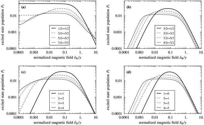
Figure 10: Excited state populations as a function of magnetic field for $J_{i}\leftrightarrow J_{i}-1$ and $J_{i}\leftrightarrow J_{i}-1$ transitions. In all cases, the rms Rabi frequency is $\Omega=\frac{\sqrt{3}}{5}\gamma$, the polarization angle $\theta_{\text{BE}}=\arccos\frac{1}{\sqrt{3}}$, and the laser detuning $\Delta=0$.

Figure 10 shows the numerically calculated total population $P_{f}$ of the $P_{J_{f}}$ levels as a function of magnetic field, with linear laser polarization and polarization angle $\theta_{\text{BE}}=\arccos\frac{1}{\sqrt{3}}$. The laser is tuned to resonance, and its intensity gives an rms Rabi frequency $\Omega=\frac{\sqrt{3}}{5}\gamma$, as in Fig. 1. The graphs in this figure all show that the excited state population is large when $\delta_{B}\sim\Omega/4$. In graph (a) of Fig. 10, the excited state populations do not vanish when $\delta_{B}$ approaches zero, since the half-integer $J_{i}\leftrightarrow J_{f}$ transitions have no dark state. However, in these transitions the excited state populations can still be increased by applying a magnetic field, especially when $J$ is large. Curves (b) – (d) display two simple scaling laws: the excited state population falls off like 1/$B^{2}$ when $\delta_{B}\gg\gamma$ because the atomic transition becomes Zeeman broadened, and it grows as $B^{2}$ in the regime $\delta_{B}\ll\gamma$ as the pumping out of the dark state(s) becomes more efficient. These three curves also show that as $J$ increases, the region in which the excited state population is large expands to include smaller values of $\delta_{B}$. This is because increasing the number of states in the system increases the time needed for optical pumping into a dark state, and so the dark state evolution rate $\delta$ can be smaller. Similarly, had the laser been detuned from resonance then the excited state population would be relatively constant over a range that includes smaller values of $\delta$, because the atom would pump into the dark states less rapidly. We find that the calculations resulting in Fig. 2 for the width and excited state population in the ${J_{i}=1}\leftrightarrow{J_{f}=0}~{}$transition give very similar results (not shown here) for these other two-level transitions.

In real atoms, large values of the total angular momentum are usually due to the presence of nuclear spin. In this case the $g$-factors of the atomic levels involved will be different than those used in Fig. 10, which mostly results in a simple shift along the $x$-axis of the appropriate curve. More importantly, when the nuclear spin is not zero the atom can be optically pumped into hyperfine levels which do not absorb light from the laser field. This leads to situations which are similar to those shown in Fig. 3, with a repumping mechanism being needed to return the atom to the light state. There are several ways of accomplishing this. Corresponding to Fig. 3(a), an rf or microwave field can drive transitions between the ground state hyperfine levels, or a second laser field can pump the atom out of the extra ground state hyperfine level through an auxiliary excited state. Corresponding to Fig. 3(b), a repumping laser field can couple the dark state to the same excited states as the main laser. For all of these cases the conclusions are the same as in the previous sections: the rate at which the atom is pumped out of the dark hyperfine level must be as large as possible without exaggerating coherence effects such as dark resonances. This means that the polarization of the radiation driving the transition out of the hyperfine states must be such that these hyperfine states do not have a stationary dark state, and that the intensity of this radiation must be great enough to drive the transition strongly. If these conditions are not met then the width of the primary transition will be broadened and the maximum scattering rate will be reduced.

It it also useful to consider the opposite limit in which optical pumping into dark hyperfine states has little effect on the scattering process because the decay rate into these states is sufficiently slow. In this case it may be possible to detect the scattered photons with a time resolution which is much smaller than the decay time to the dark hyperfine level. The dark periods following decay into the dark state can then be selectively neglected, with the result that the lineshape of the strong transition will not be broadened, in contrast to the situation discussed in Sec. IV.1.1 where only the average scattering rate was detected. Another consequence of weak coupling to a dark hyperfine state is that the Doppler-cooled atom may be able to reach equilibrium long before it decays into the dark state Berkeland:1998 . The ultimate temperature of the atom will then be the same as if the atom had only two levels (as long as the atom is not heated while it is in the dark state).

V Discussion and conclusion

In this paper we have discussed how the accumulation of atomic population in dark states can be prevented by either applying a static magnetic field or by modulating the polarization of the driving laser. We have also considered the effect of these destabilization techniques on transition lineshapes. The magnetic field technique is simple, but the more complex polarization modulation method has the important advantage of leaving the atomic energy levels unperturbed. Several different atomic systems were analyzed, and their responses to both techniques were found to be quite similar (compare Figs. 5, 9, and 10). This universal behavior arises because the evolution is always governed by the same fundamental parameters: the state evolution rate $\delta$ (given by the Zeeman shift, the AOM splitting, or the highest sideband frequency for the case of phase modulation), the Rabi frequency $\Omega$, and the excited state decay rate $\gamma$.

For a given laser intensity, the excited state population and the scattering rate are maximized by making $\delta$ comparable to $\Omega$ (typically $\delta\sim\Omega/2$). The excited state population will be small if $\Omega\gg\delta$ because the atom is then able to follow the evolving dark state adiabatically, and it will be small if $\Omega\ll\delta$, either because the laser intensity is low ($\Omega<\gamma$) or because the atom and the laser are detuned ($\delta>\gamma$). If the transition linewidth is not important, then the scattering rate can be maximized by making $\Omega$ (and $\delta$) larger than $\gamma$, so that the transition is saturated. If the linewidth is important (e.g., in laser cooling applications), then the choice $\Omega\sim\gamma/3$ gives substantial excited state population without excessive broadening. The two regimes which give small excited state population ($\Omega\gg\gamma$ and $\Omega\ll\gamma$) also result in broad lineshapes. Fortunately, the evolution rate which optimizes the excited state population also minimizes the linewidth.

If the system has more than two levels, then these rules apply to the extra transitions if they too are to remain narrow. However, often only one transition (for example, a laser cooling transition) must be narrow. In this case the extra transition should be driven as hard as possible if the system cannot form dark resonances. If the system can form dark superposition states (e.g. the ${{}^{2}S_{1/2}}\leftrightarrow{{}^{2}P_{1/2}}\leftrightarrow{{}^{2}D_{3/2}}~{}$system), then the intensities of the lasers should give Rabi frequencies such that $\Omega<\gamma/2$, to keep the dark resonances narrow. In addition, because the dark resonances occur when lasers are equally detuned from resonance, the laser frequencies can be set to keep them away from any region of interest.

- (1) G. Orriols, Nuovo Cimento 53, 1 (1979).
- (2) E Arimondo and G. Orriols, Lett. Nuovo Cimento 17, 333 (1976).
- (3) H. R. Gray, R. M. Whitley, and C. R. Stroud, Jr., Opt. Lett. 3, 218 (1978).
- (4) For a recent review, see K. Bergmann, H. Theuer, and B. W. Shore, Rev. Mod. Phys. 70, 1003 (1998).
- (5) A. Aspect, E. Arimondo, R. Kaiser, N. Vansteenkiste, and C. Cohen-Tannoudji, Phys. Rev. Lett. 61, 826 (1988).
- (6) S. E. Harris, Phys. Rev. Lett. 62, 1033 (1989).
- (7) G. Théobald, N. Dimarcq, V. Giordano and P. Cérez, Opt. Commun. 71, 256 (1989).
- (8) D. J. Wineland and H. Dehmelt, Bull. Am. Phys. Soc. 20, 637 (1975).
- (9) T. W. Hänsch and A. L. Schawlow, Opt. Commun. 13, 68 (1975).
- (10) E. Arimondo, in Progress in Optics XXXV, edited by E. Wolf (N. Holland Pub. Co, Amsterdam, 1996) p. 257.
- (11) Bruce W. Shore, The Theory of Coherent Atomic Excitation, (Wiley, New York, 1990).
- (12) G. Janik, W. Nagourney, and H. Dehmelt, J. Opt. Soc. Am. B 2, 1251-1257 (1985).
- (13) G. R. Janik, Ph.D. thesis, University of Washington – University Micro-films International, 1984.
- (14) Jon H. Shirley and R. E. Drullinger, in Conference on Precision Electromagnetic Measurements Digest, (IEEE, New York, 1994), p. 150.
- (15) G. P. Barwood, P. Gill, G. Huang, H. A. Klein, and W. R. C. Rowley, Opt. Commun. 151, 50 (1998).
- (16) D. J. Berkeland, J. D. Miller, J. C. Bergquist, W. M. Itano, and D. J. Wineland, Phys. Rev. Lett. 80, 2089 (1998).
- (17) M. Weissbluth, Atoms and Molecules (Academic Press, New York, 1978).
- (18) A. R. Edmonds, Angular Momentum in Quantum Mechanics (Princeton University Press, Princeton, NJ, 1960).
- (19) Alan A. Madej and John E. Bernard, in Frequency Measurement and Control: Advanced Techniques and Future Trends, and references therein, edited by A. Luitey (Springer-Verlag, New York, 2001).
- (20) Peter T. H. Fisk, Rep. Prog. Phys. 60, 761 (1997), and references therein.
- (21) D. A. Cardimona, M. G. Raymer, and C. R. Stroud, Jr., J. Phys. B 15, 55 (1982).
- (22) Many of the symbolic and numerical calculations presented in this paper were performed with MathematicaTM, a product of Wolfram Research, Inc., 100 Trade Center Drive, Champaign, IL, USA. Reference to this product does not imply an endorsement of the University of Sussex or Los Alamos National Laboratory.
- (23) Wayne M. Itano and D. J. Wineland, Phys. Rev. A 25, 35 (1982).
- (24) M. G. Boshier, G. P. Barwood, G. Huang, and H. A. Klein, Appl. Phys. B 71, 51 (2000).
- (25) M. Roberts, P. Taylor, S. V. Gateva-Kostova, R. B. M. Clarke, W. R. C. Rowley, and P. Gill, Phys. Rev. A 60, 2867 (1999).
- (26) V. Enders, Ph. Courteille, R. Huesmann, L. S. Ma, W. Neuhauser, R. Blatt, and P. E. Toschek, Europhysics Letters 24, 325 (1993).
- (27) P. T. H. Fisk, M. J. Sellars, M. A. Lawn and C. Coles, IEEE Trans. Ultras. Ferr. Freq. Control 44, 344 (1997).
- (28) C. Tamm, D. Schnier and A. Bauch, Appl. Phys. B 60, 19 (1995).
- (29) M. Knoop, M. Vedel, M. Houssin, T. Schweizer, T. Pawletko, and F. Vedel, in Trapped Charged Particles and Fundamental Physics, (AIP Conference Proceedings no. 457, 1999) p. 365.
- (30) S. Urabe, M. Watanabe, H. Imajo, K. Hayasaka, U. Tanaka, and R. Ohmukai, Appl. Phys. B 67, 223 (1998).
- (31) H. C. Nägerl, D. Leibfried, H. Rohde, G. Thalhammer, J. Eschner, F. Schmidt-Kaler, and R. Blatt, Phys. Rev. A 60, 145 (1999).
- (32) R. J. Hughes and D. F. W. James, Forsch. Phys. 46, 759 (1998).
- (33) M. Block, O. Rehm, P. Seibert, and G. Werth, Eur. Phys. J. D 7, 461 (1999).
- (34) J. E. Bernard, A. A. Madej, L. Marmet, B. G. Whitford, K. J. Siemsen, and S. Cundy, Phys. Rev. Lett. 82, 3228 (1999).
- (35) D. J. Berkeland “A simple linear Paul trap for Sr+” (in preparation).
- (36) R. G. DeVoe and R. G. Brewer, Phys. Rev. Lett. 76, 2049 (1996).
- (37) C. Raab, J. Bolle, H. Oberst, J. Eschner, F. Schmidt-Kaler, and R. Blatt, Appl. Phys. B 67, 683 (1998).
- (38) N. Yu, W. Nagourney, H. Dehmelt, Phys. Rev. Lett. 78, 4898 (1997).
- (39) R. Huesmann, C. Balzer, P. Courteille, W. Neuhauser, and P. E. Toschek, Phys. Rev. Lett. 82, 1611 (1999).
- (40) I. Siemers, M. Schubert, R. Blatt, W. Neuhauser, and P. E. Toschek, Europhys. Lett. 18, 139 (1992).
- (41) A. G. Sinclair, M. A. Wilson, and P. Gill, Opt. Commun. 190, 193 (2001).