Continuous quantum error correction via quantum feedback control

Abstract

We describe a protocol for continuously protecting unknown quantum states from decoherence that incorporates design principles from both quantum error correction and quantum feedback control. Our protocol uses continuous measurements and Hamiltonian operations, which are weaker control tools than are typically assumed for quantum error correction. We develop a cost function appropriate for unknown quantum states and use it to optimize our state-estimate feedback. Using Monte Carlo simulations, we study our protocol for the three-qubit bit-flip code in detail and demonstrate that it can improve the fidelity of quantum states beyond what is achievable using quantum error correction when the time between quantum error correction cycles is limited.

I Introduction

Long-lived coherent quantum states are essential for many quantum information science applications including quantum cryptography [1], quantum computation [2, 3], and quantum teleportation [4]. Unfortunately, coherent quantum states have extremely short lifetimes in realistic open quantum systems due to strong decohering interactions with the environment. Overcoming this decoherence is the chief hurdle faced by experimenters studying quantum-limited systems.

Quantum error correction is a “software solution” to this problem [5, 6]. It works by redundantly encoding quantum information across many quantum systems. The key to this approach is the use of measurements which reveal information about which errors have occurred and not about the encoded data. This feature is particularly useful for protecting the unknown quantum states that appear frequently in the course of quantum computations. The physical tools used in this approach are projective von Neumman measurements that discretize errors onto a finite set and fast unitary gates that restore corrupted data. When combined with fault-tolerant techniques, and when all noise sources are below a critical value known as the accuracy threshold, quantum error correction enables quantum computations of arbitrary length with arbitrarily small output error, or so-called fault-tolerant quantum computation [7, 8].

Quantum feedback control is also sometimes used to combat decoherence [9, 10, 11]. This approach has the advantage of working well even when control tools are limited. The information about the quantum state fed into the controller typically comes from continuous measurements and the operations the controller applies in response are typically bounded-strength Hamiltonians. The performance of the feedback may also be optimized relative to the resources that are available. For example, one can design a quantum feedback control scheme which minimizes the distance between a quantum state and its target subject to the constraint that all available controlling manipulations have bounded strengths [12].

The availability of quantum error correction, which can protect unknown quantum states, and quantum feedback control, which uses weak measurements and slow controls, suggests that there might be a way to merge these approaches into a single technique with all of these features. Previous work to account for continuous time using quantum error correction has focused on “automatic” recovery and has neglected the role of continuous measurement [13, 14, 15, 16]. On the other hand, previous work on quantum state protection using quantum feedback control has focused on protocols for known states and has not addressed the issue of protecting unknown quantum states [17, 18], however see [19] for related work.

The paper is organized as follows. In Sec. II we review quantum feedback control and introduce the formalism of stochastic master equations. In Sec. III we present the three-qubit bit-flip code as a simple example of a quantum error-correcting code and sketch the general theory using the stabilizer formalism. In Sec. IV we present our protocol for quantum error feedback control and derive an optimal non-Markovian feedback strategy for it. In Sec. V we use Monte Carlo simulations to demonstrate this strategy’s efficacy for the bit-flip code and compare it to discrete quantum error correction when the time between quantum error correction cycles is finite. Section VI concludes.

II Quantum Feedback Control

A Open quantum systems

To describe quantum feedback control, we first need to describe uncontrolled open quantum system dynamics. Let $\cal S$ be an open quantum system weakly coupled to a reservoir $\cal R$ whose self-correlation time is much shorter than both the time scale of the system’s dynamics and the time scale of the system-reservoir interaction. The Born-Markov approximation applies in this case and enables us to write down a master equation [20] describing the induced dynamics in $\cal S$:

$$\dot{\rho}=-i\left[H,\,\rho\right]+\sum_{\mu=1}^{m}{\cal{D}}[c_{\mu}]\,\rho.$$ (1)

Here $\rho$ denotes the reduced density matrix for $\cal S$, $H$ its Hamiltonian, and $\cal{D}$ a decohering Lindblad superoperator that takes a system-reservoir coupling operator (or jump operator) as an argument and acts on density matrices as

$${\cal D}[c]\rho=c\rho c^{\dagger}-{1\over 2}c^{\dagger}c\rho-{1\over 2}\rho c^{\dagger}c.$$ (2)

One way to derive this master equation is to imagine that the reservoir continuously measures the system but quickly forgets the outcomes because of rapid thermalization. The induced dynamics on $\cal S$ therefore appear as an average over all possible quantum trajectories that could have been recorded by the reservoir.

What kinds of measurements can the reservoir continuously perform? The most general measurement quantum mechanics allows is a positive operator-valued measure (POVM) $\{E_{j}\}$ acting on $\cal S$. According to a theorem by Kraus [21], the POVM $\{E_{j}\}$ can always be decomposed as

$$\sum_{i}\Omega_{ij}^{\dagger}\Omega_{ij}=E_{j},$$ (3)

such that its stochastic action is $\rho\to\rho_{j}$ with probability $p_{j}={\rm tr\thinspace}(\rho E_{j})$, where

$$\rho_{j}={1\over{\rm tr\thinspace}(\rho E_{j})}\sum_{i}\Omega_{ij}\rho\Omega_{ij}^{\dagger}.$$ (4)

This POVM is called a strong measurement when it can generate finite state changes and a weak measurement when it cannot [22]. POVMs that generate the master equation (1) involve infinitesimal changes of state, and therefore are weak measurements.

One reservoir POVM that results in the master equation (1) is the continuous weak measurement with Kraus operators

$$\Omega_{0}(dt) = 1-\left(iH+{1\over 2}\sum_{\mu=1}^{m}c_{\mu}^{\dagger}c_{\mu}\right)\,dt$$ (5)

$$\Omega_{\mu}(dt) = \sqrt{dt}\,c_{\mu},\qquad\mu=1,\ldots,m.$$ (6)

Moreover, any POVM related to the one above via the unitary rotation

$$\Omega^{\prime}_{\alpha}=\sum_{\beta}U_{\alpha\beta}\Omega_{\beta}$$ (7)

will generate the same master equation. We call each distinct POVM that generates the master equation when averaged over quantum trajectories an unravelling [23] of the master equation.

B Quantum feedback control

The previous discussion of the master equation suggests a route for feedback control. If we replace the reservoir with a device that records the measurement current, then we could feed the measurement record back into the system’s dynamics by way of a controller. For example, the master equation (1) with $m=1$ can be unravelled into the stochastic master equation (SME) [20, 24]

$$d\rho_{c}(t) = -i\left[H,\,\rho_{c}(t)\right]dt$$ (9)

$$+{\cal D}[c]\rho_{c}(t)dt+{\cal H}[c]\rho_{c}(t)dW(t)$$

$$dQ(t) = \langle{c+c^{\dagger}}\rangle^{\phantom{\dagger}}_{\!c}dt+dW(t),$$ (10)

where $\rho_{c}$ is the conditioned density matrix, conditioned on the outcomes of the measurement record $Q(t)$, the expectation $\langle{a}\rangle^{\phantom{\dagger}}_{\!c}$ means ${\rm tr\thinspace}(\rho_{c}a)$, $dW$ is a normally distributed infinitesimal random variable with mean zero and variance $dt$ (a Wiener increment [25]), and ${\cal H}$ is a superoperator that takes a jump operator as an argument and acts on density matrices as

$${\cal H}[c]\rho = c\rho+\rho c^{\dagger}-\rho\,{\rm tr\thinspace}[{c\rho+\rho c^{\dagger}}].$$ (11)

This sort of unravelling occurs, for example, when one performs a continuous weak homodyne measurement of a field $c$ by first mixing it with a classical local oscillator in a beamsplitter and then measuring the output beams with photodetectors [24]. The stochastic model (9–10) is flexible enough to incorporate other noise sources such as detector inefficiency, dark counts, time delays, and finite measurement bandwidth [26].

We can add feedback control by introducing a $Q(t)$-dependent Hamiltonian to the dynamics of $\rho_{c}$. There are two well-studied ways of doing this. The first, and simplest, is to use Wiseman-Milburn feedback [9, 24], or current feedback, in which the feedback depends only on the instantaneous measurement current $I_{Q}(t)=dQ(t)/dt$. For example, adding the Hamiltonian $I_{Q}(t)F$ to the SME (9) using current feedback leads to the dynamics [9]

$$d\rho_{c}(t) = -i\left[H,\,\rho_{c}(t)\right]dt$$ (15)

$$+{\cal D}[c]\rho_{c}(t)dt+{\cal H}[c]\rho_{c}(t)dW(t)$$

$$-i\left[F,c\rho_{c}(t)+\rho_{c}(t)c^{\dagger}\right]dt$$

$$+{\cal D}[F]\rho_{c}(t)dt-i\left[F,\rho_{c}(t)\right]dW$$

$$dQ(t) = \langle{c+c^{\dagger}}\rangle^{\phantom{\dagger}}_{\!c}dt+dW(t).$$ (16)

The second, and more general, way to add feedback is to modulate the Hamiltonian by a functional of the entire measurement record. An important class of this kind of feedback is estimate feedback [12], in which feedback is a function of the current conditioned state estimate $\rho_{c}$. This kind of feedback is of especial interest because of the quantum Bellman theorem [27], which proves that the optimal feedback strategy will be a function only of conditioned state expectation values for a large class of physically reasonable cost functions. An example of such an estimate feedback control law analogous to the current feedback Hamiltonian used in (15) is to add the Hamiltonian $\langle{I_{Q}(t)}\rangle^{\phantom{\dagger}}_{\!c}F=\langle{c+c^{\dagger}}\rangle^{\phantom{\dagger}}_{\!c}F$, which depends on what we expect the current $I_{Q}(t)$ should be given the previous measurement history rather than its actual instantaneous value. Adding this feedback to the SME (9) leads to the dynamics

$$d\rho_{c}(t) = -i\left[H,\,\rho_{c}(t)\right]dt$$ (19)

$$+{\cal D}[c]\rho_{c}(t)dt+{\cal H}[c]\rho_{c}(t)dW(t)$$

$$-i\langle{I_{Q}}\rangle^{\phantom{\dagger}}_{\!c}\left[F,\rho_{c}(t)\right]dt$$

$$dQ(t) = \langle{c+c^{\dagger}}\rangle^{\phantom{\dagger}}_{\!c}dt+dW(t).$$ (20)

III Quantum Error Correction

Although quantum feedback control has many merits, it has not been used to protect unknown quantum states from noise. Quantum error correction, however, is specifically designed to protect unknown quantum states; for this reason it has been an essential ingredient in the design of quantum computers [28, 29, 30]. The salient aspects of quantum error correction can already be seen in the three-qubit bit-flip code, even though it is not a fully quantum error correcting code. For that reason, we shall introduce quantum error correction with this example and discuss its generalization using the stabilizer formalism.

A The bit-flip code

The bit-flip code protects a single two-state quantum system, or qubit, from bit-flipping errors by mapping it onto the state of three qubits:

$$|{0}\rangle \to |{000}\rangle\equiv|{\bar{0}}\rangle$$ (21)

$$|{1}\rangle \to |{111}\rangle\equiv|{\bar{1}}\rangle.$$ (22)

The states $|{\bar{0}}\rangle$ and $|{\bar{1}}\rangle$ are called the basis states for the code and the space spanned by them is called the codespace, whose elements are called codewords.

After the qubits are subjected to noise, quantum error correction proceeds in two steps. First, the parities of neighboring qubits are projectively measured. These are the observables

$$M_{0} = ZZI$$ (23)

$$M_{1} = IZZ.$$ (24)

The error syndrome is the pair of eigenvalues $(m_{0},m_{1})$ returned by this measurement.

Once the error syndrome is known, the second step is to apply one of the following unitary operations conditioned on the error syndrome:

$$(-1,+1) \to XII$$ (25)

$$(-1,-1) \to IXI$$ (26)

$$(+1,-1) \to IIX$$ (27)

$$(+1,+1) \to III.$$ (28)

This procedure has two particularly appealing characteristics: the error syndrome measurement does not distinguish between the codewords, and the projective nature of the measurement discretizes all possible quantum errors onto a finite set. These properties hold for general stabilizer codes as well.

If the bit-flipping errors arise from reservoir-induced decoherence, then prior to quantum error correction the qubits evolve via the master equation

$$d\rho_{\mathrm{n}oise}=\gamma({\cal D}[XII]+{\cal D}[IXI]+{\cal D}[IIX])\rho\,dt,$$ (29)

where $\gamma dt$ is the probability of a bit-flip error on each qubit per time interval $[t,t+dt]$. This master equation has the solution

$$\rho(t)=$$ (34)

$$\phantom{+}a\left(t\right)\rho_{0}$$

$$+b\left(t\right)\left(XII\rho_{0}XII+IXI\rho_{0}IXI+IIX\rho_{0}IIX\right)$$

$$+c\left(t\right)\left(XXI\rho_{0}XXI+XIX\rho_{0}XIX+IXX\rho_{0}IIX\right)$$

$$+d\left(t\right)XXX\rho_{0}XXX,$$

where

$$a(t) = \left(1+3e^{-2\gamma t}+3e^{-4\gamma t}+e^{-6\gamma t}\right)/8$$ (35)

$$b(t) = \left(1+\phantom{3}e^{-2\gamma t}-\phantom{3}e^{-4\gamma t}-e^{-6\gamma t}\right)/8$$ (36)

$$c(t) = \left(1-\phantom{3}e^{-2\gamma t}-\phantom{3}e^{-4\gamma t}+e^{-6\gamma t}\right)/8$$ (37)

$$d(t) = \left(1-3e^{-2\gamma t}+3e^{-4\gamma t}-e^{-6\gamma t}\right)/8.$$ (38)

The functions $a(t)$–$d(t)$ express the probability that the system is left in a state that can be reached by zero, one, two, or three bit-flips from the initial state, respectively. After quantum error correction is performed, single errors are identified correctly but double and triple errors are not. As a result, the recovered state, averaged over all possible measurement syndromes, is

$$\rho=\left(a\left(t\right)+b\left(t\right)\right)\rho_{0}+\left(c\left(t\right)+d\left(t\right)\right)XXX\rho_{0}XXX.$$ (39)

The overlap of this state with the initial state depends on the initial state, but is at least as large as when the initial state is $|{\bar{0}}\rangle$; namely, it is at least as large as

$$F_{\bar{3}} = \left(2+3e^{-2\gamma t}-e^{-6\gamma t}\right)/4$$ (40)

$$\simeq 1-3(\gamma t)^{2}.$$ (41)

Recalling that a single qubit subject to this decoherence has error probability $p=\gamma t$, we see that, when applied sufficiently often, the bit-flip code reduces the error probability on each qubit from ${\cal O}(p)$ to ${\cal O}(p^{2})$.

B Stabilizer formalism

The bit-flip code is one of many quantum error correcting codes that can be described by the stabilizer formalism [28]. Let $\cal C$ be a $2^{k}$-dimensional subspace of a $2^{n}$-dimensional $n$-qubit Hilbert space. Then the system can be thought of as encoding $k$ qubits in $n$, where the codewords are elements of $\cal C$. Let us further define the Pauli group to be $P_{n}=\{\pm 1,\pm i\}\otimes\{I,X,Y,Z\}^{\otimes n}$, and let the weight of an operator in $P_{n}$ be the number of non-identity components it has when written as a tensor product of operators in $P_{1}$. The stabilizer of $\cal C$, $S({\cal C})$, is the group of operators which fix all codewords in $\cal C$. We call $\cal C$ an $[[n,k,d]]$ stabilizer code when ($a$) the $n-k$ generators of $S({\cal C})$ form a subgroup of $P_{n}$ and ($b$) $d$ is the smallest weight of an element in $P_{n}\setminus S({\cal C})$ that commutes with every element in $S({\cal C})$.

In this general setting, quantum error correction proceeds in two steps. First, one projectively measures the stabilizer generators to infer the error syndrome. Second, one applies a unitary recovery operator conditioned on the error syndrome. The strong measurement used in this procedure guarantees that all errors, even unitary errors, are discretized onto a finite set. For this reason we will sometimes refer to this procedure as discrete quantum error correction. When the noise rate is low and when correction is applied sufficiently often, this procedure reduces the error probability from ${\cal O}(p)$ to ${\cal O}(p^{2})$.

IV Continuous quantum error correction via quantum feedback control

In this section, we present a method for continuously protecting an unknown quantum state using weak measurement, state estimation, and Hamiltonian correction. As in the previous section, we introduce this method via the bit-flip code and then generalize.

A Bit-flip code: Theoretical model

Suppose $\rho$ is subjected to bit-flipping decoherence as in (29); to protect against such decoherence, we have seen that we can encode $\rho$ using the bit-flip code (21–22). Here we shall define a similar protocol that operates continuously and uses only weak measurements and slow corrections.

The first part of our protocol is to weakly measure the stabilizer generators $ZZI$ and $IZZ$ for the bit-flip code, even though these measurements will not completely collapse the errors. To localize the errors even further, we also measure the remaining nontrivial stabilizer operator $ZIZ$. The second part of our protocol is to apply the slow Hamiltonian corrections $XII$, $IXI$, and $IIX$ corresponding to the unitary corrections $XII$, $IXI$, and $IIX$, with control parameters $\lambda_{k}$ that are to be determined. If we parameterize the measurement strength by $\kappa$ and perform the measurements using the unravelling (9–10), the SME describing our protocol is

$$d\rho_{c} = \phantom{+}\gamma({\cal D}[XII]+{\cal D}[IXI]+{\cal D}[IIX])\rho_{c}dt$$ (46)

$$+\kappa({\cal D}[ZZI]+{\cal D}[IZZ]+{\cal D}[ZIZ])\rho_{c}dt$$

$$+\sqrt{\kappa}({\cal H}[ZZI]dW_{1}+{\cal H}[IZZ]dW_{2}$$

$$\phantom{+\kappa(}+{\cal H}[ZIZ]dW_{3})\rho_{c}$$

$$-i[F,\rho_{c}]dt$$

$$dQ_{1} = 2\kappa\langle{ZZI}\rangle^{\phantom{\dagger}}_{\!c}dt+\sqrt{\kappa}dW_{1}$$ (47)

$$dQ_{2} = 2\kappa\langle{IZZ}\rangle^{\phantom{\dagger}}_{\!c}dt+\sqrt{\kappa}dW_{2}$$ (48)

$$dQ_{3} = 2\kappa\langle{ZIZ}\rangle^{\phantom{\dagger}}_{\!c}dt+\sqrt{\kappa}dW_{3},$$ (49)

where

$$F=\lambda_{1}XII+\lambda_{2}IXI+\lambda_{3}IIX$$ (50)

is the feedback Hamiltonian having control parameters $\lambda_{k}$.

Following the logic of quantum error correction, it is natural to choose the $\lambda_{k}$ to be functions of the error syndrome. For example, the choice

$$\lambda_{1} = {\lambda\over 8}(1-\langle{ZZI}\rangle^{\phantom{\dagger}}_{\!c})(1+\langle{IZZ}\rangle^{\phantom{\dagger}}_{\!c})(1-\langle{ZIZ}\rangle^{\phantom{\dagger}}_{\!c})$$ (51)

$$\lambda_{2} = {\lambda\over 8}(1-\langle{ZZI}\rangle^{\phantom{\dagger}}_{\!c})(1-\langle{IZZ}\rangle^{\phantom{\dagger}}_{\!c})(1+\langle{ZIZ}\rangle^{\phantom{\dagger}}_{\!c})$$ (52)

$$\lambda_{3} = {\lambda\over 8}(1+\langle{ZZI}\rangle^{\phantom{\dagger}}_{\!c})(1-\langle{IZZ}\rangle^{\phantom{\dagger}}_{\!c})(1-\langle{ZIZ}\rangle^{\phantom{\dagger}}_{\!c}),$$ (53)

where $\lambda$ is the maximum feedback strength that can be applied, is reasonable: it acts trivially when the state is in the codespace and applies a maximal correction when the state is orthogonal to the codespace. Unfortunately this feedback is sometimes harmful when it need not be. For example, when the controller receives no measurement inputs (i.e., $\kappa=0$), it still adds an extra coherent evolution which, on average, will drive the state of the system away from the state we wish to protect.

This weakness of the feedback strategy suggests that we should choose our feedback more carefully. To do this, we introduce a cost function describing how far away our state is from its target and choose a control which minimizes this cost. The difficulty is that our target is an unknown quantum state. However, we can choose the target to be the codespace, which we do know. We choose our cost function, therefore, to be the norm of the component of the state outside the codespace. Since the codespace projector is $\Pi_{\cal C}=\frac{1}{4}(III+ZZI+ZIZ+IZZ)$, the cost function is $1-f$, where $f(\rho)={\mathrm{t}r}(\rho\Pi_{\cal C})$. Under the SME (46), the time evolution of $f$ due to the feedback Hamiltonian $F$ is

$$\dot{f}_{fb} = \phantom{+}2\lambda_{1}\langle{YZI+YIZ}\rangle^{\phantom{\dagger}}_{\!c}$$ (56)

$$+2\lambda_{2}\langle{ZYI+IYZ}\rangle^{\phantom{\dagger}}_{\!c}$$

$$+2\lambda_{3}\langle{ZIY+IZY}\rangle^{\phantom{\dagger}}_{\!c}.$$

Maximizing $\dot{f}_{fb}$ minimizes the cost, yielding the optimal feedback coefficients

$$\lambda_{1} = \lambda\,{\mathrm{s}gn}\langle{YZI+YIZ}\rangle^{\phantom{\dagger}}_{\!c}$$ (57)

$$\lambda_{2} = \lambda\,{\mathrm{s}gn}\langle{ZYI+IYZ}\rangle^{\phantom{\dagger}}_{\!c}$$ (58)

$$\lambda_{3} = \lambda\,{\mathrm{s}gn}\langle{ZIY+IZY}\rangle^{\phantom{\dagger}}_{\!c},$$ (59)

where, again, $\lambda$ is the maximum feedback strength that can be applied.

This feedback scheme is a bang-bang control scheme, meaning that the control parameters $\lambda_{k}$ are always at the maximum or minimum value possible ($\lambda$ or $-\lambda$, respectively), which is a typical control solution both classically [31] and quantum mechanically [32]. In practice, the bang-bang optimal controls (57) can be approximated by a bandwidth-limited sigmoid, such as a hyperbolic tangent function.

The control solution (57) requires the controller to integrate the SME (46) using the measurement currents $Q_{i}(t)$ and the initial condition $\rho_{c}$. However, typically the initial state $\rho_{c}(0)$ will be unknown. Fortunately the calculation of the feedback (57) does not depend on where the initial condition is within the codespace, so the controller may assume the maximally mixed initial condition $\rho_{e}=\frac{1}{2}(|{\bar{0}}\rangle\langle{\bar{0}}|+|{\bar{1}}\rangle\langle{\bar{1}}|)$ for its calculations. This property generalizes for a wide class of stabilizer codes, as we prove in the appendix, and we conjecture that this property holds for all stabilizer codes.

B Intuitive one-qubit picture

Before generalizing our procedure, it is helpful to gain some intuition about how it works by considering an even simpler “code”: the spin-up state (i.e., $|{0}\rangle$) of a single qubit. The stabilizer is $M_{0}=Z$, the noise it protects against is bit flips $X$, and the correction Hamiltonian is proportional to $X$. The optimal feedback, by a similar analysis to that for the bit-flip code, is $F=\lambda\,{\mathrm{s}gn}\langle Y\rangle_{c}X$, and the resulting stochastic master equation can be rewritten as a set of Bloch sphere equations as follows:

$$d\langle{X}\rangle^{\phantom{\dagger}}_{\!c} = -2\kappa\langle{X}\rangle^{\phantom{\dagger}}_{\!c}dt-2\sqrt{\kappa}\langle{X}\rangle^{\phantom{\dagger}}_{\!c}\langle{Z}\rangle^{\phantom{\dagger}}_{\!c}dW$$ (60)

$$d\langle{Y}\rangle^{\phantom{\dagger}}_{\!c} = -2\gamma\langle{Y}\rangle^{\phantom{\dagger}}_{\!c}dt-2\kappa\langle{Y}\rangle^{\phantom{\dagger}}_{\!c}-2\sqrt{\kappa}\langle{Y}\rangle^{\phantom{\dagger}}_{\!c}\langle{Z}\rangle^{\phantom{\dagger}}_{\!c}dW$$ (62)

$$-2\lambda({\mathrm{s}gn}\langle{Y}\rangle^{\phantom{\dagger}}_{\!c})\langle{Z}\rangle^{\phantom{\dagger}}_{\!c}dt$$

$$d\langle{Z}\rangle^{\phantom{\dagger}}_{\!c} = -2\gamma\langle{Z}\rangle^{\phantom{\dagger}}_{\!c}dt+2\sqrt{\kappa}(1-\langle{Z}\rangle^{2}_{\!c})dW$$ (64)

$$+2\lambda({\mathrm{s}gn}\langle{Y}\rangle^{\phantom{\dagger}}_{\!c})\langle{Y}\rangle^{\phantom{\dagger}}_{\!c}dt.$$

The Bloch vector representation $(\langle{X}\rangle,\langle{Y}\rangle,\langle{Z}\rangle)$ [3] of the qubit provides a simple geometric picture of how it evolves. Decoherence (the $\gamma$ term) shrinks the Bloch vector, measurement (the $\kappa$ terms) lengthens the Bloch vector and moves it closer to the $z$-axis, and correction (the $\lambda$ term) rotates the Bloch vector in the $y$–$z$ plane. Fig. 1 depicts this evolution: depending on whether the Bloch vector is in the hemisphere with $\langle{Y}\rangle>0$ or $\langle{Y}\rangle<0$, the feedback will rotate the vector as quickly as possible in such a way that it is always moving towards the codespace (spin-up state). Note that if the Bloch vector lies exactly on the $z$-axis with $\langle{Z}\rangle<0$, rotating it either way will move it towards the spin-up state—the two directions are equivalent, and it suffices to choose one of them arbitrarily.

FIG. 1.: Bloch sphere showing the action of our feedback scheme on one qubit. Wherever the Bloch vector is in the $y$–$z$ plane, the feedback forces it back to the spin-up state, which is the codespace of this system. All the vectors shown lie, without loss of generality, in the $x=0$ plane.

C Feedback for a general code

Our approach generalizes for a full $[[n,k,d]]$ quantum error-correcting code, which can protect against depolarizing noise [3] acting on each qubit independently. This noise channel, unlike the bit-flip channel, generates a full range of quantum errors—it applies either $X$, $Y$, or $Z$ to each qubit equiprobably at a rate $\gamma$. We weakly measure the $n-k$ stabilizer generators $\{M_{l}\}$ with strength $\kappa$. For each syndrome $m$, we apply a slow Hamiltonian correction $F_{m}$ with control strength $\lambda_{m}$, the weight of each correction being $d$ or less. The SME describing this process is

$$d\rho_{c} = \phantom{+}\gamma\sum_{j=x,y,z}\sum_{i=1}^{n}({\cal D}[\sigma^{(i)}_{j}])\rho_{c}dt+\kappa\sum_{l=1}^{n-k}{\cal D}[M_{l}]\rho_{c}dt$$ (66)

$$+\sqrt{\kappa}\sum_{l=1}^{n-k}{\cal H}[M_{l}]dW_{j}\rho_{c}-i\sum_{r=1}^{R}\lambda_{r}[F_{r},\rho_{c}]dt.$$

The number of feedback terms $R$ needed will be less than or equal to the number of errors the code corrects against. The reason that this equality is not strict is that quantum error correcting codes can be degenerate, meaning that there can exist inequivalent errors that have the same effect on the state—a purely quantum mechanical property [28].

We optimize the $\lambda_{r}$ relative to a cost function equal to the state’s overlap with the codespace. For a general stabilizer code $\cal C$, the codespace projector is

$\displaystyle\Pi_{\cal C}=\frac{1}{2^{n-k}}\prod_{l=1}^{n-k}(I+M_{l})$

and the rate of change of the codespace overlap due to feedback is

$\displaystyle\dot{f}_{fb}=-i\,{\mathrm{t}r}\sum_{r=0}^{n-k}\lambda_{r}[\Pi_{\cal C},F_{r}]\rho.$

Maximizing this overlap subject to a maximum feedback strength $\lambda$ yields the feedback coefficients

$$\lambda_{r}=\lambda\,{\mathrm{s}gn}\langle{[\Pi_{\cal C},F_{r}]}\rangle^{\phantom{\dagger}}_{\!c}.$$ (67)

This control solution, as for the bit-flip code, requires a controller to compute the feedback (67). A natural question to ask is how the scaling of the classical computation behaves. In the appendix we show that the evolution of $(2^{n-k})^{2}$ parameters must be calculated in order to compute the feedback for an $[[n,k,d]]$ code, which at first does not seem promising. However, if one encodes $mk$ qubits using $m$ copies of an $[[n,k,d]]$ code, as might well be the case for a quantum memory, the SME (66) will not couple the dynamics of the $m$ logical qubits; and, as in the bit-flip case, the initial condition for the controller’s integration can still be the completely mixed state in the total codespace. Then the relevant scaling for this system, the dependence on $m$, is linear: the number of parameters is $m(2^{n-k})^{2}$.

V Simulation of the bit-flip code

In this section, we present the results of Monte Carlo simulations of the implementation of the protocol described in Section IV for the bit-flip code.

A Simulation details

Because the bit-flip code feedback control scheme (46–49) uses a nonlinear feedback Hamiltonian, numerical simulation is the most tractable route for its study. To obtain $\rho_{c}(t)$, we directly integrated these equations using a simple Euler integrator and a Gaussian random number generator. We found stable convergent solutions when we used a dimensionless time step $\gamma dt$ on the order of $10^{-6}$ and averaged over $10^{4}$ quantum trajectories. As a benchmark, a typical run using these parameters took 2–8 hours on a 400MHz Sun Ultra 2. We found that more sophisticated Milstein [33] integrators converged more quickly but required too steep a reduction in time step to achieve the same level of stability. All of our simulations began in the state $\rho_{c}(0)=|{\bar{0}}\rangle\langle{\bar{0}}|$ because it is maximally damaged by bit-flipping noise and therefore it yielded the most conservative results.

We used two measures to assess the behavior of our bit-flip code feedback control scheme. The first measure we used is the codeword fidelity $F_{cw}(t)={\mathrm{t}r}(\rho_{c}(0)\rho_{c}(t))$, the overlap of the state with the target codeword. This measure is appropriate when one cannot perform strong measurements and fast unitary operations, a realistic scenario for many physical systems. We compared $F_{cw}(t)$ to the fidelities of one unprotected qubit $F_{1}(t)=\frac{1}{2}(1+e^{-2\gamma t})$ and of three unprotected qubits $F_{3}(t)=\left(F_{1}(t)\right)^{3}$.

The second measure we used is the correctable overlap

$$F_{corr}(t)={\mathrm{t}r}(\rho_{c}(t)\Pi_{corr}),$$ (68)

where

$$\Pi_{corr} = \phantom{+}\rho_{0}+XII\rho_{0}XII$$ (70)

$$+IXI\rho_{0}IXI+IIX\rho_{0}IIX$$

is the projector onto the states that can be corrected back to the original codeword by discrete quantum error correction applied (once) at time $t$. This measure is appropriate when one can perform strong measurements and fast unitary operations, but only at discrete time intervals of length $t$. We compared $F_{corr}(t)$ to the fidelity $F_{\bar{3}}(t)$ obtained when, instead of using our protocol up to time $t$, no correction was performed until the final discrete quantum error correction at time $t$. As we showed in equation (40), the expression for $F_{\bar{3}}(t)$ may be calculated analytically; it is $F_{\bar{3}}(t)=\frac{1}{4}(2+3e^{-2\gamma t}-e^{-6\gamma t})\sim 1-3\gamma^{2}t^{2}$.

B Results

We find that both our optimized estimate feedback scheme (57) and our heuristically-motivated feedback scheme (51) effectively protect a qubit from bit-flip decoherence. In Figs. 2 and 3 we show how these schemes behave for the (scaled) measurement and feedback strengths $\kappa/\gamma=64$, $\lambda/\gamma=128$ when averaged over $10^{4}$ quantum trajectories. Using our first measure, we see that at very short times, both schemes have codeword fidelities $F_{cw}(t)$ that follow the three-qubit fidelity $F_{3}(t)$ closely. For both schemes, $F_{cw}(t)$ improves and surpasses the fidelity of a single unprotected qubit $F_{1}(t)$. Indeed, perhaps the most exciting feature of these figures is that eventually $F_{cw}(t)$ surpasses $F_{\bar{3}}(t)$, the fidelity achievable by discrete quantum error correction applied at time $t$. In other words, our scheme alone outperforms discrete quantum error correction alone if the time between corrections is sufficiently long.

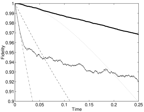
FIG. 2.: Behavior of our protocol with optimized feedback (57) for parameters $\kappa/\gamma=64$, $\lambda/\gamma=128$, averaged over $10^{4}$ quantum trajectories. The analytical curves shown are as follows: the dashed line is the fidelity of one decohering qubit, $F_{1}(t)$; the dashed-dotted line is the fidelity of three decohering qubits, $F_{3}(t)$; and the dotted line is the fidelity of an encoded qubit after one round of discrete error correction, $F_{\bar{3}}(t)$. Our simulation results are as follows: the solid line is the codeword fidelity $F_{cw}(t)$, and the thick solid line is the correctable overlap $F_{corr}(t)$.

Looking at our second measure in Figs. 2 and 3, we see that $F_{corr}(t)$ is as good as or surpasses $F_{\bar{3}}(t)$ almost everywhere. For times even as short as a tenth of a decoherence time, the effect of using our protocol between discrete quantum error correction cycles is quite noticeable. This improvement suggests that, even when one can approximate discrete quantum error correction but only apply it every so often, it pays to use our protocol in between corrections. Therefore, our protocol offers a means of improving the fidelity of a quantum memory even after the system has been isolated as well as possible and discrete quantum error correction is applied as frequently as possible.

There is a small time range from $t\cong 0.01$ to $t\cong 0.05$ for the parameters used in Fig. 2 in which using our protocol before discrete quantum error correction actually underperforms not doing anything before the correction. Our simulations suggest that the reason for this narrow window of deficiency is that, in the absence of our protocol, it is possible to have two errors on a qubit (e.g., two bit flips) that cancel each other out before discrete quantum error correction is performed. In contrast, our protocol will immediately start to correct for the first error before the second one happens, so we lose the advantage of this sort of cancellation. This view is supported by the fact that $F_{corr}(t)$ in our simulations always lies above the fidelity line obtained by subtracting such fortuitous cancellations from $F_{\bar{3}}(t)$. In any case, this window can be made arbitrarily small and pushed arbitrarily close to the beginning of our protocol by increasing the measurement strength $\kappa$ and the feedback strength $\lambda$.

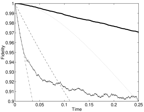
FIG. 3.: Behavior of our protocol with non-optimized feedback (51) for parameters $\kappa/\gamma=64$, $\lambda/\gamma=128$, averaged over $10^{4}$ quantum trajectories. As in Fig. 2, the dashed line is $F_{1}(t)$, the dashed-dotted line is $F_{3}(t)$, the dotted line is $F_{\bar{3}}(t)$, the solid line is $F_{cw}(t)$ and the thick solid line is $F_{cw}(t)$. Note that this feedback is qualitatively similar to that in Fig. 2 but does not perform as well.

In Figs. 2 and 3, the $F_{cw}(t)$ line is much more jagged than the $F_{corr}(t)$ line. The jaggedness in both of these lines is due to statistical noise in our simulation and is reduced when we average over more than $10^{4}$ trajectories. The reason for the reduced noise in the $F_{corr}(t)$ line has to do with the properties of discrete quantum error correction—on average, neighboring states get corrected back to the same state by discrete quantum error correction, so noise fluctuations become smoothed out.

The improvement our optimized estimate feedback protocol yields beyond our heuristically-motivated feedback protocol is more noticeable in $F_{cw}(t)$ than in $F_{corr}(t)$ as seen in Figs. 2 and 3. Our optimized protocol acts to minimize the distance between the current state and the codespace, not between the current state and the space of states correctable back to the original codeword, so this observation is perhaps not surprising. In fact, optimizing feedback relative to $F_{corr}(t)$ is not even possible without knowing the codeword being protected. Nevertheless, our optimized protocol does perform better, so henceforth we shall restrict our to discussion to it.

We investigated how our protocol behaved when the scaled measurement strength $\kappa/\gamma$ and feedback strength $\lambda/\gamma$ were varied using the two measures described in Sec. V A. Our first measure, the codeword fidelity $F_{cw}(t)$, crosses the unprotected qubit fidelity $F_{1}(t)$ at various times $\tau$ as depicted in Fig. 4. This time is of interest because it is the time after which our optimized protocol improves the fidelity of a qubit beyond what it would have been if it were left to itself. Increasing the scaled feedback strength $\lambda/\gamma$ improves our scheme and reduces $\tau$, but the dependence on the scaled measurement strength $\kappa/\gamma$ is not so obvious from Fig. 4.

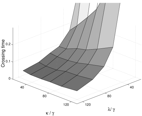
FIG. 4.: Time $\tau$ at which $F_{cw}(\tau)=F_{1}(\tau)$ as a function of measurement strength $\kappa/\gamma$ and feedback strength $\lambda/\gamma$. This crossing time is the time after which our optimized protocol improves the fidelity of a qubit beyond what it would have been if it were left to itself.

By looking at cross-sections of Fig. 4, such as at $\lambda/\gamma=80$ as in Fig. 5, we see that for a given scaled feedback strength $\lambda/\gamma$ there is a minimum crossing time $\tau$ as a function of measurement strength $\kappa/\gamma$. In other words, there is an optimal choice of measurement strength $\kappa/\gamma$. This optimal choice arises because syndrome measurements, which localize states near error subspaces, compete with Hamiltonian correction operations, which coherently rotate states between the nontrivial error subspaces to the trivial error subspace. This phenomenon is a feature of our continuous-time protocol that is not present in discrete quantum error correction; in the former, measurement and correction are simultaneous, while in the latter, measurement and correction are separate non-interfering processes.

FIG. 5.: Time $\tau$ at which $F_{cw}(\tau)=F_{1}(\tau)$ as a function of measurement strength $\kappa/\gamma$, keeping correction strength fixed at $\lambda/\gamma=80$.

In order to study how our second measure, the correctable overlap $F_{corr}(t)$, varies with $\kappa$ and $\lambda$, we found it instructive to examine its behavior at a particular time. In Fig. 6 we plot $F_{corr}(t)$, evaluated at the time $t=0.2/\gamma$, as a function of $\kappa$ and $\lambda$. As we found with the crossing time $\tau$, increasing $\lambda$ always improves performance, but increasing $\kappa$ does not because measurement can compete with correction. Since $F_{\bar{3}}(0.2/\gamma)\cong 0.927$, for all the $\kappa$ and $\lambda$ plotted in Fig. 6, using our protocol between discrete quantum error correction intervals of time $0.2/\gamma$ improves the reliability of the encoded data.

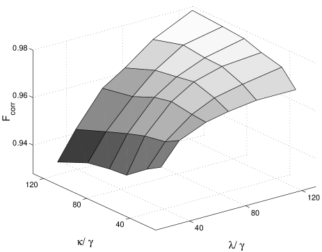
FIG. 6.: $F_{corr}$ at $\gamma t=0.2$ as a function of measurement strength $\kappa/\gamma$ and feedback strength $\lambda/\gamma$. This quantity corresponds to the fidelity of a state given continuous error-correction up to $\gamma t=0.2$, at which point discrete error-correction is performed.

VI Conclusion

In many realistic quantum computing architectures, weak measurements and Hamiltonian operations are likely to be the tools available to protect quantum states from decoherence. Moreover, even quantum systems in which strong measurements and fast operations are well-approximated, such as ion traps [34], it is likely that these operations will only be possible at some maximum rate. Our protocol is able to continuously protect unknown quantum states using only weak measurements and Hamiltonian corrections and can improve the fidelity of quantum states beyond rate-limited quantum error correction. In addition, because our protocol responds to the entire measurement record and not to instantaneous measurement results, it will not propagate errors badly and therefore has a limited inherent fault-tolerance that ordinary quantum error correction does not.

We expect that our protocol will be applicable to other continuous-time quantum information processes, such as reliable state preparation and fault-tolerant quantum computation. We also expect that our approach will work when different continuous-time measurement tools are available, such as direct photodetection. Finally, although current computing technology has limited our simulation investigation to few-qubit versions of our protocol, we are confident that many of the salient features we found in our three-qubit bit-flip code protocol will persist when our protocol is applied to larger codes.

VII Acknowledgements

We happily acknowledge helpful discussions with many colleagues, including Salman Habib, Kurt Jacobs, Hideo Mabuchi, Gerard Milburn, John Preskill, Benjamin Rahn, and Howard Wiseman. We are especially grateful to Howard Wiseman for discussions on optimizing our control scheme. This work was supported in part by the National Science Foundation under grant number EIA-0086038 and by the Department of Energy under grant number DE-FG03-92-ER40701. A. L. acknowledges support from an IBM faculty partnership award and C. A. acknowledges support from an NSF fellowship.

A Feedback based on the completely mixed state

Even though our quantum error correction feedback control scheme described in Section IV does not distinguish between codewords, it is not obvious that we do not need to know the initial codeword to integrate its SME and calculate the relevant expectation values. Since we are interested in protecting unknown quantum states, this property is crucial to our scheme’s success. Fortunately, for a large class of stabilizer codes, the computation of the feedback can be done by assuming the initial state is the completely mixed codespace state $\rho_{e}=\frac{1}{2^{n}}\prod_{l=1}^{n-k}(I+M_{l})$, which we prove here.

We begin by defining the set $G$ for the $[[n,k,d]]$ code $\cal C$ with stabilizer $S({\cal C})$ as

$$G=\left\{\alpha s\left|\,\alpha\in P_{n},s\in S({\cal C}),[s,\alpha]=0\ \mbox{iff}\ |\alpha|\ \mbox{is even}\right.\right\},$$ (A1)

where $|\alpha|$ denotes the weight of $\alpha$ as defined in section III B.

It is also useful to define the normalizer $N(S)$ for the code as the group of operators which commute with every element in $S({\cal C})$. The elements of $N(S)\setminus S$ can be thought of as the encoded operations for the code—they move one codeword to another.

We shall rewrite the conditions we require for the computation of the feedback to be insensitive to the initial codeword in terms of the Pauli basis coefficients $R_{g}(\rho)$ which we define as follows. Let $g=\sigma_{i_{1}}\otimes...\otimes\sigma_{i_{n}}$, where $i_{1}\ldots i_{n}$ take on the values $x,y,z,I$ and $\sigma_{I}=I$. Then

$$R_{g}(\rho)\equiv{\mathrm{t}r}(\rho g)/2^{n}=\langle g\rangle/2^{n},$$ (A2)

We can then formulate the problem in terms of proving conditions on $G$ as follows:

1. For every $R_{g}$ used in our feedback scheme, $g\in G$.

2. For every $g\in G$ and every $\rho_{1}$ and $\rho_{2}$ in $\cal C$, $R_{g}(\rho_{1})=R_{g}(\rho_{2})$.

3. Evolution under the SME couples members of the set $\{R_{g}|g\in G\}$ only to each other.

Theorem Let $\cal C$ be an $[[n,1,3]]$ stabilizer code whose stabilizer $S({\cal C})$ has generators of only even weight and whose encoded operations set $N(S)\setminus S$ has elements of only odd weight. Then the conditions 1–3 above are satisfied; consequently, our scheme does not require knowledge of where the initial codeword lies in $\cal C$.

Proof:

In this proof, any variable of the form $\alpha_{a}$ is an arbitrary element of $P_{n}$, and any variable of the form $s_{a}$ is an arbitrary element of $S({\cal C})$. We prove each of the conditions listed above separately.

Condition 1: By construction, $G$ contains all $M$ of the form $M=s_{i}\sigma_{j}^{(k)}$, where $[s_{i},\sigma_{j}^{(k)}]\neq 0$. These are precisely the operators used to compute the feedback in (67) for a code encoding one qubit.

Condition 2: Let $g=\alpha s\in G$ and let $\rho\in{\mathcal{C}}$. We know either $\alpha\in S$, $\alpha\in N(S)\setminus S$, or $\alpha\notin N(S)$. Suppose $\alpha\in S$. Then $g\in S$ acts trivially on all states in the codespace, so $R_{g}=1/2^{n}{\mathrm{t}r}(\rho g)=1/2^{n}$ for this case. Now suppose $\alpha\in N(S)\setminus S$. Then $[\alpha,s]=0$, and since $\alpha s\in G$, $|\alpha|$ is even. But every element of $N(S)\setminus S$ has odd weight by hypothesis, which is a contradiction. Hence $\alpha$ cannot be in $N(S)\setminus S$. Finally, suppose $\alpha\notin N(S)$. Then there exists some $s^{\prime}\in S$ such that $[\alpha,s^{\prime}]\neq 0$; let $s^{\prime}$ be such an element. Then for $|{\psi}\rangle,|{\phi}\rangle\in\cal C$,

$$\langle{\psi}|\alpha|{\phi}\rangle = \langle{\psi}|\alpha s^{\prime}|{\phi}\rangle=-\langle{\psi}|s^{\prime}\alpha|{\phi}\rangle$$ (A3)

$$= -\langle{\psi}|\alpha|{\phi}\rangle=0.$$ (A4)

Hence for this case $R_{g}=1/2^{n}{\mathrm{t}r}(\rho\alpha s)=0$. Note that these expressions for $R_{g}$ must be the same no matter where $\rho$ is in the codespace; therefore, for every $g\in G$ and $\rho_{1},\rho_{2}\in{\cal C}$, $R_{g}(\rho_{1})=R_{g}(\rho_{2})$.

Condition 3: We prove this by considering $dR_{M}$, where $M\in G$: we will show that $dR_{M}=f(\{R_{N}|N\in G\})$ for some real function $f$. Now, for any $M\in P_{n}$, $dR_{M}={\mathrm{T}r}(d\rho\ M)$, where $d\rho$ is given by the master equation (66), and we can show condition 3 for each term of the master equation separately. First, substituting in the master equation shows that any term of the form ${\cal D}[c]\rho dt$ contributes either 0 or the simple exponential damping term $-2R_{M}$ to $dR_{M}$ if $M$ and $c$ commute or anticommute, respectively.

As for the master equation term ${\cal H}[s_{j}]dW_{j}\rho$, by writing the master equation in the Pauli basis we can see that $R_{N}$ contributes to $dR_{M}$ through this term precisely when $Ns_{j}=M$ and $\{s_{j},N\}\neq 0$. Here we know that $M\in G$, so we may write $M=\alpha_{k}s_{l}$ (with the appropriate restriction on $[\alpha_{k},s_{l}]$ depending on the weight of $\alpha_{k}$) . $N=\alpha_{k}s_{l}s_{j}=\alpha_{k}s_{m}$, so the condition above that $[s_{j},N]=0$ becomes $[s_{j},\alpha_{k}s_{l}s_{j}]=(\alpha_{k}[s_{j},s_{l}s_{j}]+[s_{j},\alpha_{k}]s_{l}s_{j})$ $\Rightarrow[s_{j},\alpha_{k}]=0$. Therefore, $[\alpha_{k},s_{m}]=s_{l}[\alpha_{k},s_{j}]+[\alpha_{k},s_{l}]s_{j}=[\alpha_{k},s_{l}]s_{j}$ which is zero or not depending on the original weight of $\alpha_{k}$. So if $M=\alpha_{k}s_{l}$ is such that $M\in G$, $N=\alpha_{k}s_{m}$ must fulfill that same condition, implying that $N\in G$ also.

Similarly, $R_{N}$ contributes to $dR_{M}$ through the master equation term $[\sigma^{(k)}_{j},\rho]$ when $N\sigma_{j}^{(k)}=M$ and $[\sigma_{j}^{(k)},N]\neq 0$. Now, $M\in G$ so $M=\alpha_{l}s_{m}$, again with the appropriate restriction on $[\alpha_{l},s_{m}]$ depending on the weight of $\alpha_{l}$. Then $N=\sigma_{j}^{(k)}\alpha_{l}s_{m}\equiv\alpha_{n}s_{m}$, so the condition above that $\{\sigma_{j}^{(k)},N\}\neq 0$ becomes

$$\{\sigma_{j}^{(k)},\sigma_{j}^{(k)}\alpha_{l}s_{m}\} = \sigma_{j}^{(k)}[\sigma_{j}^{(k)},\alpha_{l}]s_{m}+\sigma_{j}^{(k)}\alpha_{l}\{\sigma_{j}^{(k)},s_{m}\}$$ (A5)

$$= \sigma_{j}^{(k)}\{\sigma_{j}^{(k)},\alpha_{l}\}s_{m}-\sigma_{j}^{(k)}\alpha_{l}[\sigma_{j}^{(k)},s_{m}]$$ (A6)

$$= 0.$$ (A7)

We can now divide the analysis of this term into two cases. Case 1 occurs when $\sigma_{j}^{(k)}\alpha_{l}$ has weight $|\alpha_{l}|$, implying that $\{\alpha_{l},\sigma_{j}^{(k)}\}=0$. Then $\{\sigma_{j}^{(k)},\sigma_{j}^{(k)}\alpha_{l}s_{m}\}=-\sigma_{j}^{(k)}\alpha_{l}[\sigma_{j}^{(k)},s_{m}]=0$, which implies that $[s_{m},\alpha_{n}]=[s_{m},\sigma_{j}^{(k)}]\alpha_{l}+\sigma_{j}^{(k)}[s_{m},\alpha_{l}]=\sigma_{j}^{(k)}[s_{m},\alpha_{l}]$. So $[s_{m},\alpha_{n}]=0$ just when $[s_{m},\alpha_{l}]=0$, which means that $N\in G$ since $|\alpha_{n}|=|\alpha_{l}|$.

In Case 2, $\sigma_{j}^{(k)}\alpha_{l}$ has weight $|\alpha_{l}\pm 1|\Rightarrow[\alpha_{l},\sigma_{j}^{(k)}]=0$. Then (A5) becomes $\{\sigma_{j}^{(k)},\sigma_{j}^{(k)}\alpha_{l}s_{m}\}=\sigma_{j}^{(k)}\alpha_{l}\{\sigma_{j}^{(k)},s_{m}\}=0$, which implies that $[s_{m},\alpha_{n}]=\{s_{m},\sigma_{j}^{(k)}\}\alpha_{l}+\sigma_{j}^{(k)}\{s_{m},\alpha_{l}\}=\sigma_{j}^{(k)}\{s_{m},\alpha_{l}\}$. So $[s_{m},\alpha_{n}]=0$ just when $\{s_{m},\alpha_{l}\}=0$, which means that $N\in G$ since $|\alpha_{n}|=|\alpha_{l}\pm 1|$. $\square$

Thus we have shown the three conditions that all the $R$’s used to compute the feedback are of the form $R_{N\in G}$; that for a given $M\in G$, $R_{M}$ will be the same for any state in the codespace; and that evolution via the master equation mixes the $R$’s of the form $R_{N\in G}$ only with each other. Therefore, we can conclude that taking the initial state to be any state in the codespace, including the true initial state and the entirely mixed state, produces the same expression for the feedback when the master equation is evolved conditioned on a measurement record, and so we do not have to know the true initial state to use our protocol.

Another consequence of using the completely mixed state for feedback arises from the fact that doing so corresponds to discarding information about the state of the system. Therefore, this procedure should reduce the number of parameters needed to compute the feedback. Unfortunately, this only leads to a modest reduction in the number of parameters, which can be found by using a simple counting argument. There are $2^{n}/2^{k}=2^{n-k}$ different error subspaces, including the no-error (code) space, and if we start with the completely mixed state in the codespace we do not need to worry at all about any movement within any of these spaces. We must only worry about which error space we are actually in, along with coherences between these spaces, so we find that $(2^{n-k})^{2}$ parameters are needed to describe the system.

REFERENCES

- [1] C. H. Bennett and G. Brassard, in Proceedings of IEEE International Conference on Computers, Systems and Signal Processing (IEEE Press, Bangalore, India, 1984), pp. 175–179, C. H. Bennett and G. Brassard, “Quantum public key distribution,” IBM Technical Disclosure Bulletin 28, 3153–3163 (1985).
- [2] M. A. Nielsen and I. L. Chuang, Quantum Computation and Quantum Information (Cambridge University Press, Cambridge, 2000).
-
[3]
J. Preskill, Lecture notes for Caltech course Ph 219: