Quantum tomography as a tool for the characterization of optical devices

Abstract

We describe a novel tool for the quantum characterization of optical devices. The experimental setup involves a stable reference state that undergoes an unknown quantum transformation and is then revealed by balanced homodyne detection. Through tomographic analysis on the homodyne data we are able to characterize the signal and to estimate parameters of the interaction, such as the loss of an optical component, or the gain of an amplifier. We present experimental results for coherent signals, with application to the estimation of losses introduced by simple optical components, and show how these results can be extended to the characterization of more general optical devices.

1 Introduction

Quantum homodyne tomography (QHT) is certainly the most successful technique for measuring the quantum state of radiation. It is based on homodyne detection, where the signal mode is amplified by the local oscillator. This means that there is no need for single-photon resolving photodetectors, whence it is possible to achieve quantum efficiency $\eta$ approaching the ideal unit value by using linear photodiodes [1]. Moreover, QHT is efficient and statistically reliable, such that it can be used on-line with the experiment. Indeed, among other proposed state reconstruction methods, QHT is the only one which has been implemented in quantum optical experiments [2, 3].

Possible applications of QHT range from the measurement of photon correlations on a sub-picosecond time-scale [2] to the characterization of squeezing properties [3, 4], photon statistics in parametric fluorescence [5], quantum correlations in down-conversion [1] and nonclassicality of states [6]. In general, the key point is that QHT provides information about the quantum state within a chosen sideband, thus allowing for a precise spectral characterization of the light beam under investigation.

In this paper we address QHT as a tool for the quantum characterization of optical devices, like the estimation of the coupling constant of an active medium or the quantum efficiency of a photodetector. The goal is to link the estimation of such parameters with the results from feasible measurement schemes, as homodyne detection, and to make the estimation procedure the most efficient. We present our experimental results about the reconstruction of the quantum state of coherent signals, together with application to the estimation of the losses introduced by simple optical components. Moreover, we show how these preliminary results can be extended to the characterization of more general optical devices.

In the next Section we review some basic elements of quantum tomography, whereas in Section 3 we describe the basic requirements needed to implement a quantum characterization tool based on tomographic measurements. In Section 4 the experimental apparatus is described with some details, and in Section 5 the experimental data are analyzed and discussed. Section 6 closes the paper by discussing the possible extensions of the present work.

2 Quantum Homodyne Tomography

Quantum tomography of a single-mode radiation field consists of a set of repeated measurements of the field-quadrature $x_{\phi}=\frac{1}{2}(ae^{-i\phi}+a^{{\dagger}}e^{i\phi})$ at different values of the reference phase $\phi$. The expectation value of a generic operator can be obtained by averaging a suitable kernel function $R[O](x,\phi)$ as follows [7]

$$\hbox{Tr}\left\{\varrho\>O\right\}=\int_{0}^{\pi}\!\!\frac{d\phi}{\pi}\int_{-\infty}^{\infty}\!\!dx\;p(x,\phi)\;R[O](x,\phi)\;,$$ (1)

where $p(x,\phi)$ denotes the probability distribution of the outcomes $x$ for the quadrature $x_{\phi}$, and $R[O](x,\phi)$ is given by

$$R[O](x,\phi)=\frac{1}{4}\int_{0}^{\infty}\!\!dr\>\hbox{Tr}\left\{O\>\cos\left[\sqrt{r}(x-{x}_{\phi})\right]\right\}\;.$$ (2)

Actually, the tomographic kernel $R[O](x,\phi)$ for a given operator $O$ is not unique, since a large class of null functions [9, 10] $F(x,\phi)$ exists that have zero tomographic average for arbitrary state. This degree of freedom can be exploited to adapt the kernel to data and achieve an optimized determination of the quantity of interest. For example, quantities like the photon number, the field amplitude and any normally ordered moment can be the tomographically estimated by averaging the following kernel

$$K[O](x,\phi)=R[O](x,\phi)+\sum_{k=0}^{M-1}\mu_{k}F_{k}(x,\phi)+\sum_{k=0}^{M-1}\mu_{k}^{*}F_{k}^{*}(x,\phi)\;,$$ (3)

where the kernels $R[O]$ for the moments are given by [11]

$$R[a^{{\dagger}}{}^{n}a^{m}](x;\phi)=e^{i(m-n)\phi}\frac{H_{n+m}(\sqrt{2}\>x)}{\sqrt{2^{n+m}}{{n+m}\choose n}}\;,$$ (4)

$H_{n}(x)$ being the Hermite polynomial of order $n$, and the null functions $F_{k}$ are expressed as $F_{k}(x,\phi)=x^{k}e^{i(k+2)\phi}\>,\>k=0,1,...$ The coefficients $\mu_{k}$ are obtained by minimizing the rms error for the given kernel on the given homodyne sample. A similar approach can be applied to optimize the reconstruction of the matrix elements $\varrho_{mn}=\langle m|\varrho|n\rangle$, thus achieving an effective quantum state characterization.

3 QHT as a tool to estimate parameters

The state reconstruction method provided by QHT is effective and reliable, such that it can be exploited to build a tool to characterize quantum devices. The general scheme for such a tool should be as follows. First, we need a stable source of quantum states, i.e. a source able to provide repeated preparations of a reference signal. The signal can be characterized by QHT, and then employed as input of a given device, which we want to characterize by the estimation of some relevant parameters. At the output, the transformed state can analyzed by QHT, such to characterize the input-output relations of the device.

In order to implement this kind of scheme two basic requirements should be satisfied: i) we need a stable source for the reference signal, and ii) an effective data processing for the tomographic samples should be devised, in order to minimize the number of measureements.

The first point can be satisfied by considering Gaussian signals, like coherent or squeezed states. Indeed, quantum signals that are most likely to be reliably generated in a lab are Gaussian states. The most general Gaussian state can be written as $\varrho=D(\mu)\,S(r)\,\nu\,S^{\dagger}(r)\,D^{\dagger}(\mu)\;,$ where $\nu$ denotes a thermal state $\nu=(n_{th}+1)^{-1}[n_{th}/(n_{th}+1)]^{a^{\dagger}a}$, $S(r)=\exp[r(a^{2}-a^{{\dagger}2})/2]$ the squeezing operator and $D(\mu)=\exp(\mu a^{\dagger}-\mu^{*}a)$ the displacement operator. However, thermal excitations can be neglected at optical frequencies, such that we may generally consider $\nu$ as the vacuum state. The homodyne distribution of the state $\varrho$ at phase $\phi$ with respect to the local oscillator is Gaussian and, remarkably, such Gaussian character is not altered by many transformations induced by optical devices, such as the loss of a component, the gain of an amplifier or the quantum efficiency of a detector. In this paper we consider the reference signal excited in a coherent state. More general signals will be considered elsewhere.

The need of an effective data processing lead to consider either adaptive or maximum-likelihood (ML) procedures on the tomographic data. In Section 5 we apply adaptive tomography for the estimation of losses induced by optical filters. Here, we illustrate the use of ML procedure to the characterization of a general (active or passive) optical media, which we plan to perform experimentally in the near future.

Let us start by reviewing the ML approach. Let $p(x|\lambda)$ the probability density of a random variable $x$, conditioned to the value of the parameter $\lambda$. The analytical form of $p$ is known, but the true value of the parameter $\lambda$ is unknown, and should be estimated from the result of a measurement of $x$. Let $x_{1},x_{2},...,x_{N}$ be a random sample of size $N$. The joint probability density of the independent random variable $x_{1},x_{2},...,x_{N}$ (the global probability of the sample) is given by

$${\cal L}(\lambda)=\Pi_{k=1}^{N}\>p(x_{k}|\lambda)\;,$$ (5)

and is called the likelihood function of the given data sample. The ML estimator of the parameter $\lambda$ is defined as the quantity $\lambda_{ML}$ that maximizes ${\cal L}(\lambda)$ for variations of $\lambda$. Since the likelihood is positive this is equivalent to maximize

$$L(\lambda)=\log{\cal L}(\lambda)=\sum_{k=1}^{N}\log p(x_{k}|\lambda)\;$$ (6)

which is the so-called log-likelihood function.

Let us consider a generic optical media: the propagation of a signal is governed, for negligible saturation effects, by the master equation

$$\dot{\varrho}=G_{1}\,L[a]\,\varrho+G_{2}\,L[a^{\dagger}]\,\varrho\;,$$ (7)

where $\varrho$ is the density matrix describing the quantum state of the signal mode $a$ and $L[O]$ denotes the Lindblad superoperator $L[O]A=O\,A\,O^{\dagger}-\frac{1}{2}O^{\dagger}O\,A-\frac{1}{2}\,A\,O^{\dagger}O$. If we model the propagation as the interaction of a traveling wave single-mode $a$ with a system of N identical two-level atoms, then the absorption $G_{1}=\gamma N_{1}$ and amplification $G_{2}=\gamma N_{2}$ parameters are related to the number $N_{1}$ and $N_{2}$ of atoms in the lower and upper level respectively. The quantity $\gamma$ is a rate of the order of the atomic linewidth [12], and the propagation gain (or deamplification) is given by ${\cal G}=\exp[(G_{2}-G_{1})\>t]$. A medium described by the master equation (7) represents a kind of phase-insensitive optical device, such that the parameters $G_{1}$ and $G_{2}$ can be estimated starting from random phase tomographic data. According to (7), the homodyne distribution of a coherent signal with initial amplitude $\alpha_{0}$ is given, after the propagation, by

$$p(x;\phi)=\frac{1}{\sqrt{\pi(\delta^{2}+g^{2}/2)}}\exp\left\{-\frac{1}{\delta^{2}+g^{2}/2}\left[x-g\hbox{Re}(\alpha_{0}\,e^{-i\phi})\right]^{2}\right\}\;.$$ (8)

with $g=e^{-Qt}$, $2Q=(G_{1}-G_{2})$, and $\delta^{2}=(G_{1}+G_{2})(1-g^{2})/4Q$ (for non-unit quantum efficiency $\eta<1$, $\delta^{2}+g^{2}/2\rightarrow\delta^{2}+g^{2}/2+(1-\eta)/2\eta)$. By ML estimation on homodyne data we may reconstruct the parameters $G_{1}$ and $G_{2}$. The resulting method has proven efficient by numerical simulations [13], and provides a precise determination of the absorption and amplification parameters of the master equation using small homodyne data sample. Notice that no advantage in using squeezed states should be expected, because of the phase-insensitive character of the device.

4 Experiment

A schematic of the experiment is presented in Fig. 1. The principal radiation source is provided by a monolithic Nd:YAG laser ($\approx$ 50 mW @1064 nm; Lightwave, model 142). The laser has a linewidth of less than 10 kHz/ms with a frequency jitter of less than 300 kHz/s, while its intensity spectrum is shot–noise limited above 2.5 MHz. The laser emits a linearly polarized beam in a TEM00 mode.

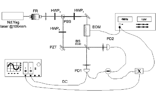
Figure 1: Schematic of the experimental set-up. A Nd:YAG laser beam is divided into two beam, one acts as the homodyne local oscillator, the other represent the signal beam. The signal is modulated at frequency $\Omega$ with a defined modulation depth to control the average photon number in the generated coherent state. The tomographic data are provided by an homodyne detector whose differece photocurrent is demodulated and then acquired by a digital oscilloscope (Tektronix TDS 520D).

The laser is protected from back reflection by a Faraday rotator (FR) whose output polarizing beam splitter can be adjusted to obtain an output beam of variable intensity. The beam outing the isolator, of $\approx$ 2.5 mW, is then split into two part of variable relative intensity by a combination of a halfwave plate (HWP₁) and a polarizing beam splitter (PBS, p–transmitted, s–reflected). The strongest part, is directly sent toward the homodyne beam–splitter (BS) where it acts as the local oscillator beam. One of the mirror in the local oscillator path is piezo mounted to obtain a variable phase difference between the two beam. The remaining part, typically less than 200 $\mu$W, is the homodyne signal. The optical paths traveled by the local oscillator and the signal beams are carefully adjusted to obtain a visibility typically above $75\%$ measured at one of the homodyne output port. The signal beam is modulated, by means of a phase electro–optic modulator (EOM, Linos Photonics PM0202), at 4MHz, and a halfwave plate (HWP₂, HWP₃) is mounted in each path to carefully match the polarization state at the homodyne input.

The basic property of the homodyne detector (described into details in Ref. [15]) is a narrow–band detection of the field fluctuations around 4MHz. The detector is composed by a 50$\div$50 beam splitter (BS), two amplified photodiodes (PD1, PD2), and a power combiner. The difference photocurrent is demodulated at 4MHz by means of an electrical mixer. In this way the detection occurs outside any technical noise and, more important, in a spectral region where the laser does not carry excess noise.

The phase modulation added to the signal beam move a certain number of photons, proportional to the square of the modulation depth, from the carrier optical frequency $\omega$ to the side bands at $\omega\pm\Omega$ so generating two few photons coherent state, with engineered average photon number, at frequencies $\omega\pm\Omega$. The sum sideband modes is then detected as a controlled perturbation attached to the signal beam [3]. The demodulated current is acquired by a digital oscilloscope (Tektronix TDS 520D) with 8 bit resolution and record length of 250000 points per run. The acquisition is triggered by a triangular shaped waveform applied to the PZT mounted on the local oscillator path. The piezo ramp is adjusted to obtain a $2\pi$ phase variation between the local oscillator and the signal beam in an acquisition window.

The homodyne data, to be used for tomographic reconstruction of the radiation state, have been calibrated according to the noise of the vacuum state. This is obtained by acquiring a set of data leaving the signal beam undisturbed while scanning the local oscillator phase. It is important to note that in case of the vacuum state no role is played by the visibility at the homodyne beam–splitter.

5 Data Analysis

Our tomographic samples consist of $N$ homodyne data $\{x_{j},\phi_{j}\}_{j=1,...,N}$ with phases $\phi_{j}$ equally spaced with respect to the local oscillator. Since the piezo ramp is active during the whole acquisition time, we have a single value $x_{j}$ for any phase $\phi_{j}$. From calibrated data we first reconstruct the quantum state of the homodyne signal. According to the experimental setup described in the previous section we expect a coherent signal with nominal amplitude that can be adjusted by varying the modulation depth of the optical mixer. However, since we do not compensate for the quantum efficiency of photodiodes in the homodyne detector ($\eta\simeq 90\%$) we expect to reveal coherent signals with reduced amplitude with respect to actual one. In addition, the amplitude is furtherly reduced by the non-maximum visibility (ranging from $75\%$ to $85\%$) at the homodyne beam–splitter.

In Fig. 2 we show a typical reconstruction, together with the reconstruction of the vacuum state used for calibration. For both states, we report the raw data, the photon number distribution, i.e. the diagonal elements $\varrho_{nn}\equiv\langle n|\varrho|n\rangle$ of the density matrix in the Fock representation, and a contour plot of the Wigner function. The matrix elements are obtained by sampling the corresponding kernel functions

$$R[\>|n\rangle\langle n+k|\>](x,\phi)=2\exp\left\{-ik\phi\right\}\sqrt{2^{k}n!(n+k)!}\>f_{nk}(x)\>,$$

where

$$f_{nk}(x)=\left\{\begin{array}[]{lr}\sum_{l=0}^{n}\frac{(-)^{l}2^{l}\Gamma(1+l+k/2)}{l!(n-l)!(l+k)!}\Phi(1+l+k/2,1/2;-2x^{2})&k\>\>\hbox{even}\\ &\\ \sum_{l=0}^{n}\frac{(-)^{l}2^{l+1/2}\Gamma(1+l+(k+1)/2)}{l!(n-l)!(l+k)!}2xe^{-2x^{2}}\Phi(-l-k/2,3/2;2x^{2})&k\>\>\hbox{odd}\end{array}\right.\>,$$

and $\Phi(a,b;x)$ denotes a confluent hypergeometric function. The tomographic determination of the matrix elements is given by the averages

$$\varrho_{nk}=\overline{R[\>|n\rangle\langle k|\>]}=\frac{1}{N}\sum_{j}R[\>|n\rangle\langle k|\>](x_{j},\phi_{j})\;,$$ (9)

whereas the corresponding confidence intervals are given (for diagonal elements) by $\delta\varrho_{nn}=\Delta\varrho/\sqrt{N}$, $\Delta\varrho$ being the rms deviation of the kernel $R$ over data (for off-diagonal elements the confidence intervals are evaluated for the real and imaginary part separately).

In order to see the quantum state as a whole, we also report the reconstruction of the Wigner function of the field, which is defined as follows

$$W(z)=\frac{2}{\pi}\hbox{Tr}\left\{\varrho\>D(2z)\>(-)^{a^{\dagger}a}\right\}\;,$$ (10)

and can be expressed in terms of the matrix elements as

$$W(z)=\mbox{Re}\sum_{d=0}^{\infty}e^{id\phi}\sum_{n=0}^{\infty}\Lambda(n,d;|z|^{2})\rho_{n,n+d}\;$$ (11)

where

$$\Lambda(n,d;|z|^{2})=(-)^{n}2(2-\delta_{d0})|2z|^{d}\sqrt{\frac{n!}{(n+d)!}}e^{-2|z|^{2}}L_{n}^{d}(|2z|^{2})\;,$$ (12)

and $L_{n}^{d}(x)$ denotes the Laguerre polynomials. Of course, the series in Eq. (11) should be truncated at some point, and therefore the Wigner function can be reconstructed only at some finite resolution.

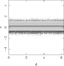
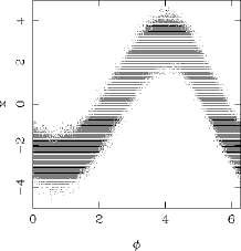
Figure 2: Reconstruction of the quantum state of the signal, and of the vacuum state used for calibration. For both states, from left to right, we report the raw data, a histogram of the photon number distribution, and a contour plot of the Wigner function. Reconstruction has been performed by a sample of $N=242250$ homodyne data. The coherent signal has an estimated average photon number equal to $\langle a^{\dagger}a\rangle=8.4$. The solid line denotes the theoretical photon distribution of a coherent state with that number of photons. Statistical errors on matrix elements are about $2\%$ . The slight phase asymmetry in the Wigner distribution corresponds to a value of about the $2\%$ of the maximum.

Once the coherence of the signal has been established we may use QHT to estimate the loss imposed by a passive optical component like an optical filter. The procedure may be outlined as follows. We first estimate the initial mean photon number $\bar{n}_{0}=|\alpha_{0}|^{2}$ of the signal beam, and then the same quantity inserting an optical neutral density filter in the signal path. If $\Gamma$ is the loss parameter, then the coherent amplitude is reduced to $\alpha_{\Gamma}=\alpha_{0}e^{-\Gamma}$, and the intensity to $\bar{n}_{\Gamma}=\bar{n}_{0}e^{-2\Gamma}$.

The estimation of the mean photon number can be performed adaptively on data by taking the average of the kernel

$$K[a^{{\dagger}}a](x)=2x^{2}-\frac{1}{2}+\mu e^{i2\phi}+\mu^{*}e^{-i2\phi}\;,$$ (13)

where $\mu$ is a parameter to be determined in order to minimize fluctuations. As proved in Ref. [10] $\mu=-1/2\langle a^{{\dagger}2}\rangle$, which itself can be obtained from homodyne data. In practice, one uses the data sample twice: first to evaluate $\mu$, then to obtain the estimate for the mean photon number.

In Fig. 3 the tomographic determinations of $\bar{n}_{\Gamma}$ are compared with the expected values for three set of experiments, corresponding to three different initial amplitudes. The expected values are given by $\bar{n}_{\Gamma}=\bar{n}_{0}e^{-2\Gamma}{\cal V}$, where $\Gamma$ is the value obtained by comparing the signal dc currents $I_{0}$ and $I_{\Gamma}$ at the homodyne photodiodes and ${\cal V=V}_{\Gamma}/{\cal V}_{0}$ is the relative visibility. The solid line in Fig. 3 denotes these values. The line is not continuos due to variations of visibility. As it is apparent from the plot the estimation is reliable in the whole range of values we could explore. It is worth noticing that the present estimation is absolute, i.e. it does not depends on the knowledge of the initial amplitude, and it is robust, since it may performed independently on the quantum efficiency of the photodiodes employed for the homodyne detector.

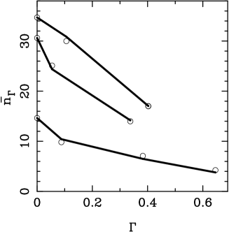
Figure 3: Estimation of the mean photon number of a coherent signal as a function of the loss imposed by an optical filter. Three set of experiments, corresponding to three different initial amplitudes are reported. Open circles are the tomographic determinations, whereas solid line denotes the expected values, as follow from nominal values of loss and visibility at the homodyne. Statistical errors are within the circles.

6 Conclusions and outlook

In this paper we addressed QHT as a tool for the characterization of quantum optical devices. We carried out the quantum state reconstruction of coherent signals, and show how QHT can be used to reliably estimate the loss imposed by an optical filter. We also show that the estimation procedure can be extended to the characterization of general (active or passive) optical devices, which we plan to perform experimentally in the near future. We also plan to extend our analysis to squeezed signals since it has been proved [14] that squeezing improves precision in the homodyne estimation of relevant parameters such the phase-shift or the quantum efficiency of a photodetector. In particular, our aim is to reproduce the described measurement scheme at the output of an OPO cavity [16] driven below threshold to generate vacuum squeezed radiation.

References

References

- [1] G. M. D’Ariano, M. Vasylìev, P. Kumar, Phys. Rev. A 58, 636 (1998).
- [2] D. F. McAlister, M. G. Raymer, Phys. Rev. A 55, R1609 (1997).
- [3] G. Breitenbach, S. Schiller, J. Mlynek, Nature 387 471 (1997); G. Breitenbach, and S. Schiller; J. Mod. Opt. 44, 2207 (1997).
- [4] M. Fiorentino, A. Conti, A. Zavatta, G. Giacomelli, F. Marin, J. of Opt. B 2, 184 (2000).
- [5] M. Vasylìev, S-K. Choi, P. Kumar, G. M. D’Ariano, Opt. Lett. 23, 1393 (1998).
- [6] G, M. D’Ariano, M. F. Sacchi, P. Kumar, Phys. Rev. A 59, 826 (1999).
- [7] G. M. D’Ariano in Quantum Communication, Computing, and Measurement, ed. by O. Hirota, A. S. Holevo, C. M. Caves (Plenum Publishing, New York 1997) p. 253.
- [8] G. M. D’Ariano, M. G. A. Paris, Phys. Rev. A, 60 518 (1999)
- [9] T. Opatrny, M. Dakna, D.-G. Welsch, Phys. Rev. A 57 2129 (1998).
- [10] G. M. D’Ariano, M. G. A. Paris, Acta Phys. Slov. 48 (1998).
- [11] Th. Richter, Phys. Lett. A 221 327 (1996).
- [12] L. Mandel and E. Wolf, Optical Coherence and Quantum Optics, (Cambridge Univ. Press, 1995).
- [13] G. M. D’Ariano, M. G. A. Paris, and M. F. Sacchi, in Quantum communication, computing, and measurements 3 p. 155, P. Tombesi and O. Hirota Eds., Kluwer/Plenum (Dordrecht, June 2001)
- [14] G. M. D’Ariano, M. G. A. Paris, M. F. Sacchi, Phys. Rev. A 62 023815 (2000).
- [15] A. Porzio, F. Sciarrino, A. Chiummo, and S. Solimeno, Opt. Comm., 194, 373 (2001).
- [16] A. Porzio, C. Altucci, M. Autiero, A. Chiummo, C. de Lisio, and S. Solimeno, ”Tunable twin beams generated by a type-I LNB OPO” in print on Appl. Phys. B.