Manifolds of interconvertible pure states

Abstract

Local orbits of a pure state of an $N\times N$ bi-partite quantum system are analyzed. We compute their dimensions which depends on the degeneracy of the vector of coefficients arising by the Schmidt decomposition. In particular, the generic orbit has $2N^{2}-N-1$ dimensions, the set of separable states is $4(N-1)$ dimensional, while the manifold of maximally entangled states has $N^{2}-1$ dimensions.
PACS numbers: 03.65.Ud; 03.67.-a

I Introduction

The existence of entangled states, i.e., roughly speaking, the states of a composite system which exhibit quantum correlations among the subsystems, appeared recently to be extremely important in rapidly developing field of quantum communication. It is due to non-classical properties of entangled states that various schemes of quantum computing, quantum cryptography and quantum teleportation can be thought of being practically realizable.

A pure state $|\psi\rangle$ in the Hilbert space ${\cal H}={\cal H}_{A}\otimes{\cal H}_{B}$ of a composite quantum system consisting of two subsystems $A$ and $B$ with Hilbert spaces ${\cal H}_{A}$ and ${\cal H}_{B}$ is separable, if it can be cast to the product form $|\psi\rangle=|\psi_{A}\rangle\otimes|\psi_{B}\rangle$, where $|\psi_{A}\rangle$ and $|\psi_{B}\rangle$ are some states of the subsystems. States which are not separable are called entangled. The situation is more complicated in the case of a mixed state (a density matrix $\rho$) [1]. It is separable if it is expressible as a convex sum of product states: $\rho=\sum_{i}p_{i}\rho_{i}^{(A)}\otimes\rho_{i}^{(B)}$, $p_{i}>0$, $\sum_{i}p_{i}=1$, where $\rho_{i}^{(A)}$ and $\rho_{i}^{(B)}$ are, in general mixed, states of the subsystems. A mixed state is called entangled if it is not separable. In what follows we consider only systems with finite-dimensional Hilbert spaces which seem to be more important in proposed applications of quantum information theory, the infinite-dimensional case needs some refinement of the above definition of separability.

It is relatively easy to check whether a given pure state is separable or entangled (e.g. by investigating its Schmidt coefficients - see below). The situation complicates for mixed states - we do not know how to check unambiguously separability of a given mixed states if the dimensionality of the Hilbert spaces of subsystems exceeds $3$ [2].

As a problem complementary to determining the separability properties of a given state one can pose the question of the relation between the set of the separable (entangled) states to the set of all states of the composite system. This can be understood as the question of a relative measure of the set of entangled states (i.e. ”how probable is that a given state is entangled?”) - the problem posed and partially solved in [3, 4], or about the geometrical and topological properties of this set. In this paper we concentrate on the latter problem in the following setting. Since we are interested in quantum correlations between two subsystems we should take into consideration only these properties which do not change under various quantum mechanical operations performed locally in each subsystem. Thus two states which are interconvertible one to another via local unitary transformations (i.e. purely quantum mechanical operations without decoherence) are equivalent from the point of their entanglement properties. This can lead to construction of appropriate measures of entanglement characterizing the classes of equivalent states. Our approach is in a sense complementary to the task of identifying the set of all invariants with respect to the local unitary transformations [5, 6, 7, 8, 9, 10, 11].

In this work we pose and solve the question of the dimensionality and topology of manifolds of states equivalent to a given one via local unitary transformations. Thus the present paper may be regarded as an extension of [12] (see also [13, 14, 15]), in which these questions were discussed for the simplest system of two qubits. In the case of pure states we find the explicit results for any $N\times N$ composite system by identifying explicitly the topology of the orbits as well as in a purely algebraic, algorithmic manner. The second approach which does not depend on the Schmidt decomposition (see below) is, in principle, applicable also to mixed states, this is illustrated by considering the generalized Werner states [1].

II Pure entangled states

A Schmidt decomposition

Consider a pure state $|\psi\rangle$ of a composite Hilbert space ${\cal H}={\cal H}_{A}\otimes{\cal H}_{B}$ of size $N^{2}$. Introducing an orthonormal basis $\{|n\rangle\}_{n=1}^{N}$ in each subsystem, we may represent the state as

$$|\psi\rangle=\sum_{n=1}^{N}\sum_{m=1}^{N}C_{mn}|n\rangle\otimes|m\rangle.$$ (1)

The complex matrix of coefficients $C$ of size $N$ needs not to be Hermitian nor normal. Its singular values (i.e. the square roots of eigenvalues $\lambda_{k}$ of the positive matrix $C^{\dagger}C$) determine the Schmidt decomposition [16, 17, 18]

$$|\psi\rangle=\sum_{k=1}^{N}\sqrt{\lambda_{k}}|k^{\prime}\rangle\otimes|k^{\prime\prime}\rangle,$$ (2)

where the basis in $\cal H$ is transformed by a local unitary transformation $W\otimes V$. Thus $|k^{\prime}\rangle=W|k\rangle$, and $|k^{\prime\prime}\rangle=V|k\rangle$, where $W$ and $V$ are the matrices of eigenvectors of $C^{\dagger}C$ and $CC^{\dagger}$, respectively. In the generic case of a non-degenerate vector $\Lambda$, the Schmidt decomposition is unique up to two unitary diagonal matrices, up to which the matrices of eigenvectors $W$ and $V$ are determined. The normalization condition $\langle\psi|\psi\rangle=1$ enforces $\sum_{k=1}^{N}\lambda_{k}=1$. Thus the vector ${\Lambda}=(\lambda_{1},...,\lambda_{N})$ lives in the ($N-1$) dimensional simplex ${\cal S}_{N}$. The Schmidt coefficients $\lambda_{k}$ do not depend on the initial basis $|n\rangle\otimes|m\rangle$, in which the analyzed state $|\psi\rangle$ is represented.

B Pure state entanglement

The Schmidt coefficient of a pure state $|\psi\rangle$ are equal to the eigenvalues of the reduced density operator, obtained by partial tracing, $\rho^{A}={\rm tr}_{B}(|\psi\rangle\langle\psi|)$. A pure state is called separable, if it can be represented in the product form $|\psi\rangle=|\psi_{A}\rangle\otimes|\psi_{B}\rangle$, where $|\psi_{A}\rangle\in{\cal H}_{A}$ and $|\psi_{B}\rangle\in{\cal H}_{B}$. This occurs if and only if there exists only one non-zero Schmidt coefficient, $\lambda_{1}=1$, i.e. the reduced state $\rho^{A}$ is pure. In the opposite case state $|\psi\rangle$ is called entangled. A pure state is called maximally entangled if all its Schmidt coefficients are equal, $\lambda_{1}=\lambda_{k}=1/N$. Note that the Schmidt coefficients are invariant with respect to any local operations $U_{L}=U_{A}\otimes U_{B}$, and thus they may serve as ingredients of any measure of entanglement.

C Local orbits

We are going to study the orbits of a given pure state $|\psi\rangle$ with respect to the local transformations $U_{L}$. Two states belonging to the same orbit are called interconvertible, since they may be reversibly transformed by local transformations one into another [19]. Let us order its Schmidt coefficients $\Lambda=(0\leq\lambda_{1}\leq\lambda_{2}\leq\cdots\leq\lambda_{N})$. In order to describe the character of the degeneracy we rename them into $\Lambda=(0,\cdots,0,\nu_{1},\cdots,\nu_{1},\nu_{2},\cdots,\nu_{2},\dots,\nu_{K},\cdots,\nu_{K})$ where each value $\nu_{n}$ occurs $m_{n}$ times and $m_{0}$ is the number of vanishing Schmidt coefficients. Obviously $m_{0}+\sum_{n=1}^{K}m_{n}=N$, and $m_{0}$ might be equal to zero. The main result of our paper is contained in the following

Proposition. The local orbit generated from $|\psi\rangle$ has the structure of the following quotient space

$${\cal O}=\frac{U(N)\times U(N)}{{\mathcal{G}}(m_{0},m_{1},\ldots,m_{K})},$$ (3)

where ${\mathcal{G}}(m_{0},m_{1},\ldots,m_{K})$ is the subgroup of the direct product $U(N)\times U(N)$ consisting of the pairs of unitary matrices $(U,V)$ of the form

$$U=\left[\begin{array}[]{cccc}u_{0}&&&\\ &u_{1}&&\\ &&\ddots&\\ &&&u_{K}\end{array}\right],\quad V=e^{i\phi}\left[\begin{array}[]{cccc}v_{0}&&&\\ &u_{1}^{*}&&\\ &&\ddots&\\ &&&u_{K}^{*}\end{array}\right],$$ (4)

where $u_{0}$ and $v_{0}$ arbitrary matrices from $U(m_{0})$, and $u_{1},\ldots,u_{K}$ denote arbitrary matrices from, respectively, $U(m_{1}),\ldots,U(m_{K})$. The overall phase factor $e^{i\phi}$ accounts for the irrelevant phase of the state $|\psi\rangle$, ie. we identify states differing by a phase factor. The dimension of the orbit (3) reads

$${\rm dim}({\cal O})=2N^{2}-2m_{0}^{2}-\sum_{n=1}^{K}m_{n}^{2}-1\ .$$ (5)

Indeed, let us observe that the action of the tensor product $U\otimes V\in U(N)\otimes U(N)$ on the state (1),

$$U\otimes V|\psi\rangle=\sum_{m,n}C_{mn}U|m\rangle\otimes V|n\rangle=\sum_{m,n,k,l}C_{mn}U_{km}|k\rangle\otimes V_{ln}|l\rangle=\sum_{k,l}(UCV^{T})_{kl}|k\rangle\otimes|l\rangle,$$ (6)

reduces to the direct product action on the coefficient matrix $C$

$$U(N)\times U(N)\ni(U,V):C\mapsto(U,V)(C):=UCV^{T}$$ (7)

Let now the action of $(\tilde{U},\tilde{V})$ reduces $C$ to its diagonal Schmidt form

$$\tilde{U}C\tilde{V}^{T}=\text{diag}(0,\ldots,0,\nu_{1},\ldots,\nu_{2},\ldots,\nu_{K},\ldots,\nu_{K}).$$ (8)

Then $\tilde{U}C\tilde{V}^{T}=U\tilde{U}C\tilde{V}^{T}V^{T}$ iff $U$ and $V$ are given by (4) Now the formula (3) follows in an obvious manner, once we realize that in fact we should disregard any unimportant overall phase of (1) (or in other words we should identify the coefficient matrices $C$ and $C^{\prime}=e^{i\theta}C$, ie. work in an appropriate projective space). The dimension formula (5) follows from a simple calculations involving the dimensionalities of the unitary groups, while the last term equal to unity stems from the projectivisation procedure. An alternative, algebraic proof of this result is proved in Section III.

In fact the orbit has a structure of a Cartesian product:

$${\cal O}=\frac{U(N)}{U(m_{0})\times U(m_{1})\times\cdots\times U(m_{K})}\times\frac{U(N)}{U(m_{0})\times U(1)},$$ (9)

where the first factor represents global orbits in the set of density matrices of size N with the same spectrum [20, 21]. In the language of fiber bundles such orbits form the base, while the fibers consists of all $N\times N$ pure states, which are related by partial tracing to a given density matrix of size $N$. We shall provide a complete proof of this fact elsewhere [22].

In the generic case of all coefficients different (and non zero), i.e. $K=N$ the manifold is thus identified as

$${\cal O}_{g}=\frac{U(N)}{[U(1)]^{N}}\times\frac{U(N)}{U(1)},$$ (10)

with the dimension

$${\rm dim}({\cal O}_{g})=2N^{2}-N-1\ .$$ (11)

The set of all orbits enumerated above produces the complex projective space ${\mathbb{C}}P^{N^{2}-1}$ - the $(2N^{2}-2)$ dimensional manifold of pure states of the $N\times N$ system. However, the the set constructed of the generic orbits (11) generated by each point of the interior of the Weyl chamber, is of full measure in the space of pure states. In this way we demonstrated a foliation of ${\mathbb{C}}P^{N^{2}-1}$. This foliation is singular, since there exist also (measure zero) leaves of various dimensions and topology, as listed in Table 1 for $N=2,3$ and $4$.

D Special cases: separable and maximally entangled states

For separable states there exists only one non zero coefficient, $\lambda_{1}=1$, so $m_{0}=N-1$. Thus (3) gives

$${\cal O}_{\rm sep}=\frac{U(N)}{U(1)\times U(N-1)}\times\frac{U(N)}{U(1)\times U(N-1)}={\mathbb{C}}P^{N-1}\times{\mathbb{C}}P^{N-1},$$ (12)

with the dimension ${\rm dim}({\cal O}_{\rm sep})=4(N-1)$. The maximally entangled states are characterized by $\lambda_{1}=\lambda_{N}=1/N$, hence $m_{1}=N$ and $m_{0}=0$. Therefore

$${\cal O}_{\rm max}=\frac{U(N)}{U(1)}=\frac{SU(N)}{Z_{N}},$$ (13)

with the dimension ${\rm dim}({\cal O}_{max})=N^{2}-1$. Note that this space is not isomorphic with $SU(N)$ because $U(N)$ is not a direct product of $U(1)$ and $SU(N)$ [23]. Since $SU(N)\times U(1)=U(N)\times Z_{N}$, where $Z_{N}$ is the discrete permutation group of $N$ elements, the orbit of the maximally entangled states can be written as ${\cal O}_{\rm max}=SU(N)/Z_{N}$. This structure follows also from the fact that the entire orbit may be written as ${\cal O}_{\rm max}=(U\otimes{\mathbb{I}})|\Psi\rangle$, where $|\Psi\rangle$ is an arbitrary maximally entangled state, and U is an arbitrary unitary matrix determined up to an overall phase [24].

E Special cases: $N=2,3$ and $4$

The set of all possible Schmidt vectors $\Lambda$ form the $N-1$ dimensional simplex ${\cal S}_{N}$. Its corners represent $N$ mutually orthogonal separable states, while its center denotes the maximally entangled state $|\psi_{*}\rangle=(\sum_{k=1}^{N}|kk\rangle)/\sqrt{N}$. Any permutation of the Schmidt coefficients may be obtained by a local transformation of the pure state. Therefore it is sufficient to consider the orbits generated by Schmidt vectors belonging to a certain asymmetric part ${\tilde{\cal S}}_{N}$ of the simplex, so called Weyl chamber. Any ordering of the Schmidt coefficients corresponds to choosing one chamber out of $N!$, in which the simplex ${\cal S}_{N}$ can be decomposed.

The Schmidt simplex and exemplary Weyl chamber for $N=2,3$ and $4$ are presented in Fig.1. (Note that the simplex of diagonal density matrices of size $N$, obtained from $N\times N$ pure states by partial tracing, has the same geometry). The numbers by each part of the boundary of ${\tilde{\cal S}}_{N}$ denote the dimensions of the local orbits, which are listed in Table 1. In the simplest case $N=2$ the simplex reduces to the interval $[0,1]$, while its asymmetric part ${\tilde{\cal S}}_{2}$ equals to $[0,1/2]$. The edge $0$ generates the four dimensional orbit of separable states, ${\mathbb{C}}P^{1}\times{\mathbb{C}}P^{1}$, and the point $1/2$ leads to the $3$–D manifold of maximally entangled states ${\cal O}_{\rm max}=SU(2)/Z_{2}\approx SO(3)\approx{\mathbb{R}}P^{3}$. This structure was pointed out by Vollbrecht and Werner [24], and the above singular foliation of ${\mathbb{C}}P^{3}$ was discussed in [12, 13, 14, 15]. In the case of any point inside the simplex (12) gives the following topology of the generic $2\times 2$ local orbit

$${\cal O}_{g}=\frac{U(2)}{U(1)^{2}}\times\frac{U(2)}{U(1)}=S^{2}\times{\mathbb{R}}P^{3},$$ (14)

in agreement with recent results of Mosseri and Dandoloff [15].

III Algebraic determination of orbit dimension

A General case: $N\times N$ mixed states

The reasoning presented in the previous section hinges on the Schmidt decomposition of the density matrix for a pure state. As such it cannot be extended to mixed states. For this reason we present an alternative method introduced in [12], which can be, in principle, applied also in the latter situation. It is based on purely algebraic reasoning, and, as such, gives only local information, i.e. only about the dimensions of the manifolds of interconvertible states and not about their topology.

Although the group of local unitary transformations is ${\mathcal{L}}=U(N)\otimes U(N)$, it is obvious that since its elements act on an arbitrary density matrix $\rho\in{\mathbb{C}}^{N}\otimes{\mathbb{C}}^{N}$ by conjugations, $\rho\mapsto U\rho U^{\dagger}$, we can take in fact ${\mathcal{L}}=SU(N)\otimes SU(N)$ instead. Let ${\mathbb{R}}^{2(N^{2}-1)}\ni{\mathbf{s}}\mapsto U({\mathbf{s}})\in SU(N)\otimes SU(N)$ be some parameterization of the group ${\mathcal{L}}$ such that $U(0)=I$ (i.e. ${\mathbf{s}}=\left(s_{1},s_{2},\ldots,s_{2N^{2}-2}\right)$ are the coordinates in $SU(N)$ with the origin at the unit matrix). The tangent space to the local orbit through $\rho$ (i.e. to the space of the states interconvertible with $\rho$) at this point is spanned by the vectors:

$$\rho_{k}:=\frac{\partial}{\partial s_{k}}U({\mathbf{s}})\rho U^{\dagger}({\mathbf{s}})\left.\right|_{{\mathbf{s}}=0}.$$ (15)

The dimension of the tangent space, hence of the manifold itself, equals the number of linearly independent vectors $\rho_{k}$.

From the unitarity of $U({\mathbf{s}})$ it follows:

$$\rho_{k}=\left[\left(\frac{\partial U}{\partial s_{k}}\right)_{{\mathbf{s}}=0},\rho\right]=\left[l_{k},\rho\right]=\rho_{k}^{\dagger}.$$ (16)

The number of independent $\rho_{k}$ equals the rank of the $2(N^{2}-1)\times 2(N^{2}-1)$ Gram matrix (the unimportant factor of $1/4$ is introduced for further convenience)

$$G_{mn}:=\frac{1}{4}{\mathrm{T}r}\rho_{m}\rho_{n},$$ (17)

which, upon using (16), can be cast into:

$$G_{mn}=\frac{1}{2}Tr\left({l_{m}\rho l_{n}\rho}\right)-\frac{1}{4}Tr\left({\rho^{2}\left\{{l_{n}l_{m}+l_{m}l_{n}}\right\}}\right).$$ (18)

Choosing the standard parameterization of $SU(N)$ in the vicinity of the identity we obtain

$$l_{k}:=\left(\frac{\partial U}{\partial s_{k}}\right)_{{\mathbf{s}}=0}=\left\{\begin{array}[]{cc}ie_{k}\otimes I,&k=1,\ldots,N^{2}-1\\ iI\otimes e_{k},&k=N^{2},\ldots,2N^{2}-2,\end{array}\right.$$ (19)

where $e_{k}=-e_{k}^{\dagger}$ are generators of the Lie algebra ${\mathfrak{s}u}(N)$. They obey the commutation relations

$$[e_{j},e_{k}]=c_{jkl}e_{l},$$ (20)

where $c_{jkl}$ denote the structure constants and we use the summation convention. We normalize $e_{k}$ to fulfill

$${\mathrm{T}r\,}e_{j}e_{k}=-2\delta_{jk}.$$ (21)

An arbitrary hermitian matrix $\rho$ acting in ${\mathbb{C}}^{N}\otimes{\mathbb{C}}^{N}$ can be decomposed with the help of ${\mathfrak{s}u}(N)$ generators

$$\rho:=\frac{1}{N^{2}}I+ia_{k}(e_{k}\otimes I)+ib_{l}(I\otimes e_{l})+C_{mn}(e_{m}\otimes e_{n}).$$ (22)

From (16), (19), (20), (21), and (22) the Gram matrix (17) is calculated as

$$G=\left[\begin{array}[]{lr}A&B\\ B^{T}&D\end{array}\right],$$ (23)

where the $(N^{2}-1)\times(N^{2}-1)$ matrices $A,B$, and $D$ read

$$A_{mn} = c_{mjk}c_{nlk}(Na_{j}a_{l}+2C_{jr}C_{lr})/2,$$ (24)

$$B_{mn} = c_{mjk}c_{nlr}C_{kl}C_{jr},$$ (25)

$$D_{mn} = c_{mjk}c_{nlk}(Nb_{j}b_{l}+2C_{rj}C_{rl})/2.$$ (26)

B Special case: $N\times N$ pure states

Using the above outlined procedure we can recover the results for pure states obtained in Section I. For a pure state $\rho=\left|\psi\right\rangle\left\langle\psi\right|$ Eq. (18) reduces to

$$G_{mn}=\left\langle\psi\right|l_{m}\left|\psi\right\rangle\left\langle\psi\right|l_{n}\left|\psi\right\rangle-\frac{1}{2}\left\langle\psi\right|l_{m}l_{n}+l_{n}l_{m}\left|\psi\right\rangle\left\langle\psi|\psi\right\rangle.$$ (27)

We choose the following explicit form of the generators $e_{k}$ expressed in the standard basis $\{\left|1\right\rangle,\left|2\right\rangle,\cdots,\left|N\right\rangle\}$ of ${\mathbb{C}}^{N}$

$$e_{k}=-i\sqrt{\frac{2}{{k(k+1)}}}\left({k\left|k+1\right\rangle\left\langle k+1\right|-\sum\limits_{l=1}^{k}{\left|l\right\rangle}\left\langle l\right|}\right),\quad k=1,2,\ldots,N-1,$$ (28)

$$e_{mn}^{(1)}=i(\left|n\right\rangle\left\langle m\right|+\left|m\right\rangle\left\langle n\right|),\quad 1\leq m<n\leq N,$$ (29)

$$e_{mn}^{(2)}=\left|n\right\rangle\left\langle m\right|-\left|m\right\rangle\left\langle n\right|,\quad 1\leq m<n\leq N.$$ (30)

We reorder the non-diagonal generators $e_{mn}^{(1)}$ and $e_{mn}^{(2)}$ by changing two indices $\{mn\}$ into a single one $k$ according to $k=N-1+(m-1)N-m(m+1)/2+n$ in the case of $e_{mn}^{(1)}$ and $k=N-1+N(N-1)/2-m(m+1)/2+n$ in the case of $e_{mn}^{(2)}$, so that $\{e_{k}\}$, $k=1,2,\ldots,N^{2}-1$ is the desired complete set of generators.

It proves to be more convenient to use not $l_{k}$ themselves, but the following linear combinations of them:

$$L_{k} := i(e_{k}\otimes I+I\otimes e_{k})/2,\quad 1\leq k\leq N^{2}-1,$$ (31)

$$L_{k} := i(e_{k}\otimes I-I\otimes e_{k})/2,\quad N^{2}\leq k\leq 2N^{2}-2,$$ (32)

what amounts to a mere change of basis in the Lie algebra and, obviously, does not influence the rank of $G$.

After rather straightforward but lengthy calculation we find $G$ in the form (23) with $B=0$ and bloc-diagonal matrices $A$ and $D$

$$A=\left[\begin{array}[]{lr}A^{(1)}&0\\ 0&A^{(2)}\end{array}\right],\quad D=\left[\begin{array}[]{lr}D^{(1)}&0\\ 0&D^{(2)}\end{array}\right].$$ (37)

The blocks $A^{(2)}$ and $D^{(2)}$ are diagonal $(N^{2}-N)\times(N^{2}-N)$ matrices with the diagonal entries

$$A^{(2)}_{kk} = (\sqrt{\lambda_{m}}+\sqrt{\lambda_{n}})^{2}\left(\sum_{j=1}^{N}\lambda_{j}\right),\quad 1\leq k\leq(N^{2}-N)/2,$$ (38)

$$A^{(2)}_{kk} = (\sqrt{\lambda_{m}}-\sqrt{\lambda_{n}})^{2}\left(\sum_{j=1}^{N}\lambda_{j}\right),\quad(N^{2}-N)/2<k\leq N^{2}-N,$$ (39)

$$D^{(2)}_{kk} = (\sqrt{\lambda_{m}}-\sqrt{\lambda_{n}})^{2}\left(\sum_{j=1}^{N}\lambda_{j}\right),\quad 1\leq k\leq(N^{2}-N)/2,$$ (40)

$$D^{(2)}_{kk} = (\sqrt{\lambda_{m}}+\sqrt{\lambda_{n}})^{2}\left(\sum_{j=1}^{N}\lambda_{j}\right),\quad(N^{2}-N)/2<k\leq N^{2}-N,.$$ (41)

In each of the above formulas $(m,n)$ is the unique pair of numbers such that $0<m<n\leq N$ and fulfilling $(m-1)N-m(m+1)/2+n=k$ for $1\leq k\leq(N^{2}-N)/2$ or $(m-1)N-m(m+1)/2+n=k-(N^{2}-N)/2$ for $(N^{2}-N)/2<k\leq N^{2}-N$. Moreover, we find that of two $(N-1)\times(N-1)$ matrices $A^{(1)}$ and $D^{(1)}$ the latter equals zero, while the former reads

$$A^{(1)}_{mn} = \frac{{\left({\sum\nolimits_{k=1}^{m}{\lambda_{k}-m\lambda_{m+1}}}\right)\left({\sum\nolimits_{k=1}^{N}{\lambda_{k}}}\right)-\left({\sum\nolimits_{k=1}^{m}{\lambda_{k}-m\lambda_{m+1}}}\right)\left({\sum\nolimits_{k=1}^{n}{\lambda_{k}-n\lambda_{n+1}}}\right)}}{{\sqrt{m(m+1)n(n+1)}}}=A^{(1)}_{nm},\quad m<n,$$ (42)

$$A^{(1)}_{nn} = \frac{{\left({\sum\nolimits_{k=1}^{n}{\lambda_{k}+n^{2}\lambda_{n+1}}}\right)\left({\sum\nolimits_{k=1}^{N}{\lambda_{k}}}\right)-\left({\sum\nolimits_{k=1}^{n}{\lambda_{k}-n\lambda_{n+1}}}\right)^{2}}}{{n(n+1)}}\,.$$ (43)

In this way we found that the entire matrix $G$ has at least $N-1$ vanishing eigenvalues (due to $D^{(1)}=0$), $N^{2}-N$ doubly degenerate eigenvalues $(\lambda_{i}\pm\lambda_{j})^{2}$ (the eigenvalues of $A^{(2)}$ and $D^{(2)}$) and the $N-1$ eigenvalues of $A^{(1)}$.

Although, at first sight, $A^{(1)}$ looks quite complicated, it is relatively easy to calculate the traces of its powers $\text{Tr}(A^{(1)})^{k}$, $k=1,2,\ldots,N-1$ and, consequently, its characteristic polynomial

$$P\left(\lambda\right):=\text{det}(A^{(1)}-\lambda)=\sum_{k=1}^{N}\left(-1\right)^{k+1}kp_{k}\lambda^{N-k}.$$ (44)

Here $p_{1}=\tau_{1}$, $p_{2}=\tau_{2}$, and $p_{k}=\tau_{k}\left(\sum_{j=1}^{N}\lambda_{j}\right)^{k-2}$ where $\tau_{k}$ are the coefficients of

$$Q\left(\lambda\right):=\prod_{i=1}^{N}\left(\lambda-\lambda_{i}\right)=\sum_{k=1}^{N}\left(-1\right)^{k}\tau_{k}\lambda^{N-k},$$ (45)

i.e. the elementary symmetric polynomials in $\lambda_{1},\lambda_{2},\ldots,\lambda_{N}$ of the order $k$. Observe that due to the normalization $\sum_{k=1}^{N}\lambda_{k}=1$ we can substitute $\tau_{k}$ for $p_{k}$ in (44) and, consequently,

$$P\left(\lambda\right)=\sum_{k=1}^{N}\left(-1\right)^{k+1}kp_{k}\lambda^{N-k}=\lambda Q^{\prime}\left(\lambda\right)-NQ\left(\lambda\right),$$ (46)

where $Q^{\prime}\left(\lambda\right):={dQ\left(\lambda\right)}/{d\lambda}$. It follows immediately that the multiplicity of the root $\lambda=0$ in $P$ equals the multiplicity of $\lambda=0$ in $Q$ (i.e. the number of Schmidt coefficients equal to $0$). Indeed, if $Q(\lambda)=\lambda^{k}Q_{1}(\lambda)$ and $Q_{1}(0)\neq 0$ then $Q^{\prime}(\lambda)=k\lambda^{k-1}Q_{1}(\lambda)+\lambda^{k}Q_{1}^{\prime}(\lambda)$ and $P(\lambda)=\lambda^{k}\left[(k-N)Q_{1}(\lambda)+\lambda Q_{1}^{\prime}(\lambda)\right]=\lambda^{k}P_{1}(\lambda)$, where $P_{1}(0)=(k-N)Q_{1}(0)\neq 0$ since $k\leq N$.

Now we are ready to calculate the rank of $G$. There are

1. $N-1$ vanishing eigenvalues of $D^{(1)}$,

2. $m_{0}$ vanishing eigenvalues of $A^{(1)}$,

3. for each $m_{n}$-degenerate Schmidt coefficient $m_{n}(m_{n}-1)$ vanishing eigenvalues of $A^{(2)}$ of the form (39) and of the form (40) of $D^{(2)}$,

4. $2m_{0}(m_{0}-1)$ vanishing eigenvalues of $A^{(2)}$ and $D^{(2)}$ of the forms (38–41).

hence the co-rank (the number of zero eigenvalues of $G$) equals $(N-1)+m_{0}+\sum_{n=1}^{K}(m_{n}^{2}-m_{n})+2(m_{0}^{2}-m_{0})=2m_{0}^{2}+\sum_{n=1}^{K}m_{n}^{2}$-1, where we used $m_{0}+\sum_{n=1}^{K}m_{n}=N$. Consequently, taking in account that $G$ is an $2(N^{2}-1)\times 2(N^{2}-1)$ matrix, its rank equal to the dimension of the orbit is given by (5).

As mentioned at the beginning of the section, the above analysis can be, in principle, extended to mixed states. To show this let’s consider (admittedly rather trivial) example of the generalized Werner states

$$\rho=\frac{1-\alpha}{N}I+\alpha|\psi\rangle\langle\psi|,$$ (47)

where the pure state $|\psi\rangle$ is characterized by the Schmidt numbers $(0\leq\lambda_{1}\leq\lambda_{2}\leq\cdots\leq\lambda_{N})$. It is obvious that the $\rho_{k}$ of Eq. (16) are, up to the scaling factor $\alpha$ the same as for the pure state $|\psi\rangle$. Consequently, the dimension of the orbit through $\rho$ is determined by the Schmidt coefficients of $|\psi\rangle$ exactly in the same way as previously.

IV Coefficients of the characteristic polynomials as entanglement measures

There exist several non equivalent ways to quantify quantum entanglement [25, 26, 27]. Following Vedral and Plenio [28] we assume that any entanglement measure

i) equals to zero for any separable state,

ii) is invariant with respect to local unitary operations,

iii) cannot increase under operations involving local measurements and classical communication.

For pure states, $\rho=|\psi\rangle\langle\psi|$, these requirements are fulfilled by the Shannon entropy of the Schmidt vector, (in other words von Neumann entropy of the partially reduced density matrix), $E_{1}(|\psi\rangle)=-\sum_{k=1}^{N}\lambda_{k}\ln\lambda_{k}$, simply called entropy of entanglement, as well as the generalized Renyi entropies, $E_{\alpha}(|\psi\rangle)={\mathrm{l}n}(\sum_{k=1}^{N}\lambda_{k}^{\alpha})/(1-\alpha)$ [29, 30].

Consider now the coefficients $\tau_{k}$ of the characteristic polynomial (44) of the nontrivial block $A^{(1)}$ of the Gram matrix (27) for a pure state of a $N\times N$ bipartite system. As derived above they are given by the elementary symmetric polynomials in $\lambda_{1},\lambda_{2},\ldots,\lambda_{N}$ of the order $k$

$$\tau_{1} = \sum_{k=1}^{N}\lambda_{k}=1,$$ (48)

$$\tau_{2} = \sum_{k=1}^{N}\sum_{l=k+1}^{N}\lambda_{k}\lambda_{l},$$ (49)

$$\tau_{3} = \sum_{k=1}^{N}\sum_{l=k+1}^{N}\sum_{m=l+1}^{N}\lambda_{k}\lambda_{l}\lambda_{m},$$ (50)

$$... ...$$ (51)

$$\tau_{N} = \prod_{k=1}^{N}\lambda_{k}.$$ (52)

Due to the definition of the Gram matrix the coefficients $\tau_{k}$, $k=2,\dots,N$ are invariant with respect to local unitary transformations and are equal to zero if and only if the state is separable.

As shown recently by Nielsen [31] any pure state $|\psi\rangle$ may be transformed locally into a given state $|\phi\rangle$, if and only if the corresponding vectors of the Schmidt coefficients satisfy the following majorization relation ${\vec{\lambda}}_{\psi}\prec{\vec{\lambda}}_{\phi}$. Any entanglement measure cannot increase under such an operation. This condition is fulfilled by the coefficients $\tau_{k}$, since the elementary symmetric polynomials are known to be Schur–concave functions [32], for which ${\vec{\lambda}}\prec{\vec{\mu}}$ induces $\tau({\vec{\lambda}})\geq\tau({\vec{\mu}})$. Thus the quantities (48) posses the property of entanglement monotones, and their set consisting of $N-1$ independent elements, $\{\tau_{2},\dots\tau_{N}\}$, provides the complete characterization of the pure states entanglement [29]. Beside the simplest case of $N=2$, (for which all measures of the entanglement generate the same order in the set of pure states [30]), the coefficients $\tau_{k}$ are not functions of the Renyi entropies and induce different orders in the set of pure entangled states.

It might be interesting to analyze how the traces of the Gram matrix, $t_{k}:={\mathrm{t}r}(G^{k})$, change during non-unitary local transformations. Our numerical experiments performed for mixed states of $2\times 2$ system suggest that all traces $t_{k}$, $k=1,\ldots,6$ do not increase under local bistochastic transformations , $\rho\mapsto\rho^{\prime}=\sum_{i}p_{i}U_{i}^{A}\otimes U_{i}^{B}\rho U_{i}^{A\dagger}\otimes U_{i}^{B\dagger}$, with $\sum_{i}p_{i}=1$. The question whether this property holds also for systems of higher dimensions remains open.

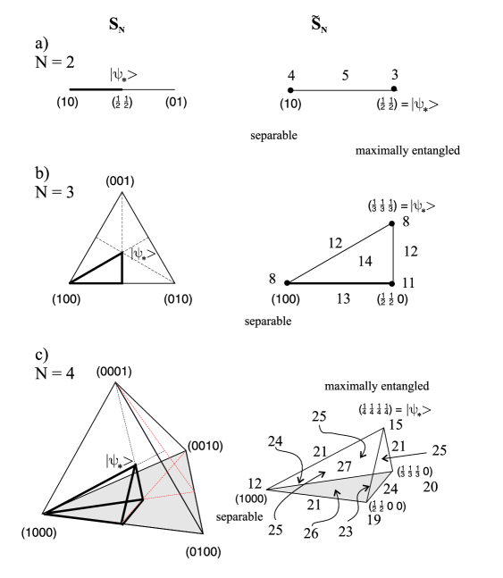
FIG. 1.: Simplex of Schmidt coefficients $S_{N}$ for pure states of $N\times N$ system with $N=2,3$, and $4$; (the same picture may also represent the set of the spectra of density matrices of size $N$ obtained from pure states by partial tracing). Right hand side shows an asymmetric part of $S_{N}$ - the Weyl chamber ${\tilde{S}}_{N}$, while the numbers denote the dimensionality of local orbits generated by each point.

$N$	Schmidt	$D_{s}$	Part of the	Topological Structure				$D_{o}$
	coefficients		asymmetric simplex	base		fibre
	$(a,b)$	$1$	line	$\frac{U(2)}{[U(1)]^{2}}$	$\times$	$\frac{U(2)}{U(1)}$	$=S^{2}\times{\mathbb{R}}P^{3}$	$5$
$2$	$(1,0)$	$0$	left edge ( $\circ$ )	$\frac{U(2)}{[U(1)]^{2}}$	$\times$	$\frac{U(2)}{U(1)\times U(1)}$	$={\mathbb{C}}P^{1}\times{\mathbb{C}}P^{1}$	$4$
	$(1/2,1/2)$	$0$	right edge ( $\star$ )	$\frac{U(2)}{U(2)}$	$\times$	$\frac{U(2)}{U(1)}$	$=\frac{SU(2)}{Z_{2}}={\mathbb{R}}P^{3}$	$3$
	$(a,b,c)$	$2$	interior of triangle	$\frac{U(3)}{[U(1)]^{3}}$	$\times$	$\frac{U(3)}{U(1)}$		$14$
	$(a,b,0)$	$1$	base	$\frac{U(3)}{[U(1)]^{3}}$	$\times$	$\frac{U(2)}{U(1)\times U(1)}$		$13$
$3$	$(a,b,b)$	$1$	2 upper sides	$\frac{U(3)}{U(1)\times U(2)}$	$\times$	$\frac{U(3)}{U(1)}$		$12$
	$(1/2,1/2,0)$	$0$	right corner	$\frac{U(3)}{U(2)\times U(1)}$	$\times$	$\frac{U(3)}{U(1)\times U(1)}$		$11$
	$(1,0,0)$	$0$	left corner ( $\circ$ )	$\frac{U(3)}{U(1)\times U(2)}$	$\times$	$\frac{U(3)}{U(2)\times U(1)}$	$={\mathbb{C}}P^{2}\times{\mathbb{C}}P^{2}$	$8$
	$(1/3,1/3,1/3)$	$0$	upper corner ( $\star$ )	$\frac{U(3)}{U(3)}$	$\times$	$\frac{U(3)}{U(1)}$	$=\frac{SU(3)}{Z_{3}}$	$8$
	$(a,b,c,d)$	$3$	interior of tetrahedron	$\frac{U(4)}{[U(1)]^{4}}$	$\times$	$\frac{U(4)}{U(1)}$		$27$
	$(a,b,c,0)$	$2$	base face	$\frac{U(4)}{[U(1)]^{4}}$	$\times$	$\frac{U(4)}{[U(1)]^{2}}$		$26$
	$(a,a,b,c)$	$2$	three upper faces	$\frac{U(4)}{U(2)\times[U(1)]^{2}}$	$\times$	$\frac{U(4)}{U(1)}$		$25$
	$(a,a,b,0)$	$1$	2 edges of the base	$\frac{U(4)}{U(2)\times[U(1)]^{2}}$	$\times$	$\frac{U(4)}{U(1)\times U(1)}$		$24$
$4$	$(a,a,b,b)$	$1$	edge	$\frac{U(4)}{[U(2)]^{2}}$	$\times$	$\frac{U(4)}{U(1)}$		$23$
	$(a,a,a,b)$	$1$	2 edges	$\frac{U(4)}{U(3)\times U(1)}$	$\times$	$\frac{U(4)}{U(1)}$		$21$
	$(a,b,0,0)$	$1$	lower edge of the base	$\frac{U(4)}{[U(1)]^{2}\times U(2)}$	$\times$	$\frac{U(4)}{U(2)\times U(1)}$		$21$
	$(1/3,1/3,1/3,0)$	$0$	back corner	$\frac{U(4)}{U(3)\times U(1)}$	$\times$	$\frac{U(4)}{U(1)\times U(1)}$		$20$
	$(1/2,1/2,0,0)$	$0$	right corner	$\frac{U(4)}{[U(2)]^{2}}$	$\times$	$\frac{U(4)}{U(2)\times U(1)}$		$19$
	$(1/4,1/4,1/4,1/4)$	$0$	upper corner ( $\star$ )	$\frac{U(4)}{U(4)}$	$\times$	$\frac{U(4)}{U(1)}$	$=\frac{SU(4)}{Z_{4}}$	$15$
	$(1,0,0,0)$	$0$	left corner ( $\circ$ )	$\frac{U(4)}{U(1)\times U(3)}$	$\times$	$\frac{U(4)}{U(3)\times U(1)}$	$={\mathbb{C}}P^{3}\times{\mathbb{C}}P^{3}$	$12$

Table 1.  Topological structure of local orbits of the $N\times N$  pure states generated by one Weyl chamber of the simplex of the Schmidt coefficients, $D_{s}$ is the dimension of the subspace, while $D_{o}$ represents the dimension of the orbit, ( $\circ$ ) denotes separable states, while ( $\star$ ) denotes maximally entangled states.

REFERENCES

• [1] R. F. Werner, Phys. Rev. A 40, 4277 (1989).
• [2] M. Lewenstein, D. Bruß, J. I. Cirac, B. Kraus, M. Kuś, A. Sanpera, R. Tarrach, and J. Samsonowicz, J. Mod. Opt.  47, 2481 (2000).
• [3] K. Życzkowski, P. Horodecki, A. Sanpera, and M. Lewenstein, Phys. Rev. A 58, 883 (1998).
• [4] K. Życzkowski, Phys. Rev. A 60, 3496 (1999).
• [5] N. Linden, S. Popescu and A. Sudbery, Phys. Rev. Lett. 83, 243 (1999).
• [6] M. Grassl, M. Rötteler, and T. Beth, Phys. Rev. A 58, 1833 (1998).
• [7] B.-G. Englert and N. Metwally, J. Mod. Opt. 47 2221 (2000).
• [8] H. A. Carteret and A. Sudbery, J. Phys. A 33, 4981 (2000).
• [9] Y. Makhlin, arXiv preprint quant-ph/0002045.
• [10] S. J. Lomonaco, arXiv preprint quant-ph/0101120.
• [11] S. Albeverio and S-M. Fei, arXiv preprint quant-ph/0109073.
• [12] M. Kuś and K. Życzkowski, Phys. Rev. A 63, 032307 (2001).
• [13] D. C. Brody, L. Hughston, J. Geom. Phys. 38, 19 (2001).
• [14] I. Bengtsson, J. Brännlund, K. Życzkowski, arXiv preprint quant-ph/0108064
• [15] R. Mosseri and Dandoloff, arXiv preprint quant-ph/0108137
• [16] E. Schmidt, Math. Annalen 63, 433 (1906).
• [17] A. Peres, Quantum Theory: Concepts and Methods, Kluver, Dordrecht 1993.
• [18] A. Ekert and P. L. Knight, Am. J. Phys. 63, 415 (1995).
• [19] D. Jonathan and M. B. Plenio, Phys. Rev. Lett. 83, 3566 (1999).
• [20] M. Adelman, J. V. Corbett and C. A. Hurst, Found. Phys. 23, 211 (1993).
• [21] K. Życzkowski and W. Słomczyński, J. Phys. A 34, 6689 (2001).
• [22] M. Kuś et al to be published
• [23] L. Michel, Rev. Mod. Phys. 52, 617 (1980).
• [24] K. G. H. Vollbrecht and R. F. Werner, J. Math. Phys. 41, 6772, (2000).
• [25] M. Horodecki, P. Horodecki and R. Horodecki, Phys. Rev. Lett. 84, 2014 (2000).
• [26] S. Virmani and M. B. Plenio, Phys. Lett. A 268, 31 (2000).
• [27] M. J. Donald, M. Horodecki, and O. Rudolph, arXiv preprint quant-ph/0105017.
• [28] V. Vedral and M. B. Plenio, Phys. Rev. A 57, 1619 (1998).
• [29] G. Vidal, J. Mod. Opt. 47, 355 (2000).
• [30] K. Życzkowski and I. Bengtsson, arXiv preprint quant-ph/0103027 and Ann. Phys. (N.Y.) (2001) in press.
• [31] M. A. Nielsen, Phys. Rev. Lett. 83, 436 (1999).
• [32] A. W. Marshall and I. Olkin, Inequalities: Theory of Majorization and its Applications, Academic Press, New York 1979.
Refer to caption