Reflections upon separability and distillability

Abstract

We present an abstract formulation of the so-called Innsbruck-Hannover programme that investigates quantum correlations and entanglement in terms of convex sets. We present a unified description of optimal decompositions of quantum states and the optimization of witness operators that detect whether a given state belongs to a given convex set. We illustrate the abstract formulation with several examples, and discuss relations between optimal entanglement witnesses and $n$-copy non-distillable states with non-positive partial transpose.

I I. Introduction

The characterization and classification of entangled states, introduced by Schrödinger Sch:35 , is perhaps the most challenging open problem of modern quantum theory. There are at least four important issues that motivate us to study the entanglement problem:

I. Interpretational and philosophical motivation: Entanglement plays an essential role in apparent “paradoxes” and counter-intuitive consequences of quantum mechanics EPR:35 ; Sch:35 ; Zurek .

II. Fundamental physical motivation: The characterization of entanglement is one of the most fundamental open problems of quantum mechanics. It should answer the question what the nature of quantum correlations in composite systems Per:95 is.

III. Applied physical motivation: Entanglement plays an essential role in applications of quantum mechanics to quantum information processing (quantum computers qcomp , quantum cryptography qcrip and quantum communication qcomm ). The resources needed to implement a particular protocol of quantum information processing are closely linked to the entanglement properties of the states used in the protocol. In particular, entanglement lies at the heart of quantum computing.

IV. Fundamental mathematical motivation: The entanglement problem is directly related to one of the most challenging open problems of linear algebra and functional analysis: the characterization and classification of positive maps on ${\cal C}^{*}$ algebras posmaps1 ; jami ; posmaps2 ; posmaps3 .

In the recent years there have been several excellent reviews treating the entanglement problem, i.e. the question whether a given state is entangled and if it is, how much entangled it is. Considerable effort has been also devoted to the distillability problem, i.e. the question whether one can distill a maximally entangled state from many copies of a given state, by means of local operations and classical communication. Entanglement is discussed in the context of quantum communication in hororev . B. Terhal summarizes the use of witness operators for detecting entanglement in terhal . Various entanglement measures are presented in the context of the theorem of their uniqueness in mdonald . Some of us have recently written a “primer” primer , which aims at introducing the non-expert reader to the problem of separability and distillability of quantum states, an even more elementary “tutorial” tutor , and a partial “tutorial” tutor1 .

The present paper, which contains material of invited lectures given by Dagmar Bruß and Maciej Lewenstein at the Second Conference on “Quantum Information Theory and Quantum Computing”, held by the European Science Foundation in Gdańsk in July 2001, is not yet another review or tutorial. It is addressed to experts in the area and reports the recent progress in the applications of the so-called Innsbruck-Hannover (I-Ha) programme of investigations of quantum correlations and entanglement (see Fig. 1 for the logo of the programme). The new results of the present paper are as follows. First, we present an abstract formulation of the I–Ha programme in terms of convex sets. Second, we present a unified description of optimal decompositions of quantum states and optimization of witness operators that detect whether a given state belongs to a given convex set. We illustrate the abstract formulation with several examples, and point out analogies and differences between them. Finally, we discuss relations between optimal entanglement witnesses and $n$-copy non-distillable states with non-positive partial transpose.

Figure 1: Logo of the I–Ha programme.

The paper is organized as follows. In section II we briefly present the milestones in the investigations of the separability problem. Then, in section III we present the abstract formulation of the I-Ha programme, and discuss such concepts as optimal decompositions, edge states, witness operators and their optimization, and canonical forms of witnesses and linear maps. Several applications are presented in section IV; they concern the questions of separability of quantum states, Schmidt number of quantum states and classification of mixed states in three-qubit systems. Furthermore we discuss relations between optimal witnesses and non-distillable states with non-positive partial transpose (NPPT states)barbara . We conclude in section V.

II II. Milestones in the separability problem

The separability problem can be formulated in simple words as follows: Given a physical state in a many-party system described by a density operator, is it separable, i.e. can it be prepared by local actions and classical communication, or not? Mathematically, this question reduces to the question whether the state $\varrho$ can be written as convex combination of projectors onto product states; for two-party systems a mixed state $\varrho$ is called separable iff it can be written as wer

$$\varrho\,{=}\,\sum_{i}p_{i}|\,e_{i}\rangle\langle e_{i}\,|\otimes|\,f_{i}\rangle\langle f_{i}\,|\ ,$$ (1)

otherwise it is entangled. Here the coefficients $p_{i}$ are probabilities, i.e. $0\leq p_{i}\leq 1$ and $\sum_{i}p_{i}=1$. Note that in general neither $\{|e_{i}\rangle\}$ nor $\{|f_{i}\rangle\}$ have to be orthogonal.

It is relatively easy to detect whether a given pure state is entangled or not, since only the simple tensor product states are separable. An appropriate tool to investigate this in two-party systems is provided by the Schmidt decomposition Per:95 . It is also known that entangled pure states incorporate genuine quantum correlations, can be distilled and violate some kind of Bell’s inequalities ???? . The situation is completely different for mixed states, where up to now we cannot answer the question of separability of a given state in general.

For the perspective of the present paper, we can point out the following milestones in the investigations of the separability problem foot :

• The mathematical definition of separable states and its suprising consequences for Bell inequalities has been given by Reinhard Werner in 1989 wer .

• Following the mixed states teleportation idea Popescu0 the first scheme of how to improve entanglement of a spatially mixed state is provided by Sandu Popescu Popescu (significantly extended by Nicolas Gisin with the help of the POVM technique gisin ).

• In 1996 the IBM group pur has given first examples of purification and distillation procedures and related them to quantum error correcting codes (applied by the Oxford group to quantum privacy amplification oxf ).

• In 1996 Asher Peres peres has formulated the necessary condition for separability that requires positivity of the partial transpose.

• In the same year 1996 it has been proven that the PPT condition is also sufficient in $2\otimes 2$ and $2\otimes 3$ systems in Ref. ppt . In the same paper the relation of the separability problem to the theory of positive maps has been rigorously formulated.

• First examples of entangled states with positive partial transpose in higher dimensions (PPTES) have been found in pawel . Here a necessary condition for separability based on the analysis of the range of the state in question (the so-called “range” criterion) has been formulated as well.

• Since 1998 PPT entanglement has been identified in a series of papers as non–distillable, but sometimes activable; this type of entanglement has been termed “bound entanglement” horodist ; horobe ; horoact ; reduction .

• In 1998 the I-Ha programme was initiated with the first paper on optimal decompositions M&A .

• Several families of PPTES’s were constructed by the IBM group, using a systematic procedure based on unextendible product bases (UPBs) UPB .

• Barbara Terhal presented in 2000 the first construction of non-decomposable entanglement witnesses (nd-EW) and non-decomposable positive maps (nd-PM) related to UPBs witness .

• In 2000 the existence of non–distillable states with non–positive partial transpose (non–distillable NPPT states) has been conjectured by us npt1 and by the IBM group npt2 .

The I–Ha programme initially concentrated on the separability problem for two-party systems. Only recently its scope has enlarged and incorporated studies of multi-party systems, continuous variables (CV) systems, and systems of identical particles. This has led us to an abstract general formulation of the I-Ha programme which we present in the next section. In this and the following section we provide the necessary references when we discuss concrete applications of the I–Ha programme.

III III. Innsbruck–Hannover programme

This section is divided into several subsections that describe the abstract formulation of the I–Ha programme, as well as successive elements of the programme: optimal decompositions, edge states, witness operators and their optimization. We present here for the first time the optimization procedure as a form of optimal decomposition of witness operators and discuss canonical forms of witnesses and corresponding linear maps.

III.1 Abstract formulation of the problem

The problem that we consider is schematically represented in Fig. 2. We consider two sets of self-adjoint operators $S_{1}$ and $S_{2}$ acting on a Hilbert space $H=H_{A}\otimes H_{B}\otimes\ldots$ of some composite quantum system. We denote the space of operators acting on $H$ by ${\cal B}(H)$. This is a Hilbert space with the scalar product induced by the trace operation. Both sets $S_{1}$ and $S_{2}$ are compact, i.e. closed and bounded, and convex. The set $S_{1}$ is a proper subset of $S_{2}$. In many applications those sets are subsets of the set of physical operators, i.e. they contain trace class, positive operators of trace one. We will consider, however, also the case when the sets $S_{1}$ and $S_{2}$ will contain witness operators, which by definition are not positive definite, although they are trace class and have trace one. We will assume that the properly defined identity operator belongs to $S_{1}$. For Gaussian states in systems with continuous variables the states will be represented by their correlation matrices, and the sets $S_{1}$ and $S_{2}$ will be the sets of correlation matrices of certain properties. In this latter case, the sets $S_{1}$ and $S_{2}$ will be closed and convex, but not necessarily bounded. Quite generally we assume that the sets are invariant under local invertible operations.

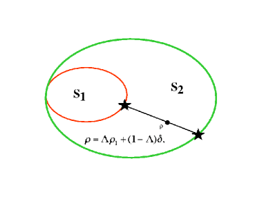
Figure 2: Scheme of the abstract formulation of the problem.

The class of questions that we consider is: Given $\varrho\in S_{2}$, does it belong to $S_{1}$, or not?

III.2 Optimal decomposition

A useful tool to study such questions is provided by the optimal decomposition:
Theorem 1. Every $\varrho\in S_{2}$ can be decomposed as a convex combination of an operator $\varrho_{1}\in S_{1}$ and $\delta\in S_{2}\setminus S_{1}$,

$$\varrho=\Lambda\varrho_{1}+(1-\Lambda)\delta,$$ (2)

where $1\geq\Lambda\geq 0$. The above decomposition is optimal in the sense that $\delta$ can only have a trivial decomposition with the corresponding $\Lambda=0$. There exists the best decomposition, for which $\Lambda$ is maximal and unique.

The proof of the above Theorem is the same as the proof of the similar theorem discussed in the context of separability and PPTES’s M&A ; karnas . Note that the optimal decomposition is not unique, and that when $\Lambda=1$ then $\varrho\in S_{1}$. The coefficient $\Lambda$ corresponding to the best decomposition is unique, but generally it is not known if the best decomposition is. So far, this has been proven only for the best separable decompositions for $2\otimes 2$ systems in Ref. M&A and for $M\otimes N$ systems in Ref. karnas . Note also that optimal decompositions can be obtained in a constructive way, by subtracting from $\varrho$ operators in $S_{1}$, keeping the remainder in $S_{2}$. It is sufficient to subtract $\varrho_{1}\in S_{1}$ that are extremal points of the convex set $S_{1}$.

III.3 Edge operators

The operators $\delta$ that enter the optimal decompositions are called edge operators. They are defined as follows:
Definition 1. A state $\delta\in S_{2}$ is an edge operator iff for every $\varrho_{1}\in S_{1}$ and $\epsilon>0$ the operator $\varrho^{\prime}=(1+\epsilon)\delta-\epsilon\varrho_{1}$ does not belong to $S_{2}$.

Note that the edge operators characterize fully the operators that belong to $S_{2}\setminus S_{1}$, and every extremal point of the convex set $S_{2}$ is either an element of $S_{1}$, or an edge operator. The construction of examples of edge operators is possible by constructing optimal decompositions. It is usually possible to check constructively if a given operator is an edge operator.

III.4 Witnesses and their optimization

The existence of witness operators is a direct consequence of the Hahn–Banach theorem rudin . Witness operators are defined as follows:
Definition 2. An operator $W$ is a witness operator (pertaining to the pair of sets $S_{1}$ and $S_{2}$) iff for every $\sigma\in S_{1}$ it holds that ${\rm Tr}(\sigma W)\geq 0$, and there exists a $\varrho\in S_{2}$ for which ${\rm Tr}(\varrho W)<0$. We say that $W$ detects $\varrho$. We normalize the witnesses demanding that ${\rm Tr}(W)=1$.

For every $\varrho\in S_{2}\setminus S_{1}$ there exists a witness operator which detects it. Witness operators in the context of the separability problem, i.e. entanglement witnesses have been discussed already in the seminal paper ppt . In the recent years first examples of the so-called non–decomposable entanglement witnesses were provided by B. Terhal terhal who introduced the name “entanglement witness”. Terhal’s construction provides witnesses of PPT entangled states that are obtained from UPBs. The most general procedure of constructing decomposable and non-decomposable entanglement witnesses was provided by us char ; opti .

Non-trivial entanglement witnesses are operators that have some negative eigenvalues. However, the positivity of mean values on product states leads to additional non-trivial properties. To illustrate this we shall present here the proof of some property which was known for specialists (see for example tutor1 ) but the proof of it has nowhere been published explicitely.
Observation. If $W_{A}$ and $W_{B}$ stand for partial reductions of $W$ then the range of $W$ belongs to tensor products of ranges of the reductions.

Note that the above property is possessed by all bipartite states (see bechan ) but not by all operators (see the operator $|\Psi_{+}\rangle\langle\Psi_{+}|-\frac{1}{2}|0\rangle|0\rangle\langle 0|\langle 0|$ with the triplet wavefunction $|\,\Psi_{+}\rangle$). To prove the Observation it is only needed to show that $P_{W_{A}}\otimes IWP_{W_{A}}\otimes I=W$, where $P_{W_{A}}$ stands for the projection on the support of $W_{A}$. We have to prove (i) $P_{W_{A}}^{\perp}\otimes IWP_{W_{A}}^{\perp}\otimes I=0$ and (ii) $P_{W_{A}}^{\perp}\otimes IWP_{W_{A}}\otimes I=P_{W_{A}}\otimes IWP_{W_{A}}^{\perp}\otimes I=0$. Let $|e\rangle\in P_{W_{A}}$ and $|e\rangle^{\perp}\in P_{W_{A}}^{\perp}$. Then by the very definition $\langle e^{\perp}|\langle f|W|e^{\perp}\rangle|f\rangle\geq 0$. The same inequality holds for all $|f^{\prime}\rangle$-s that form an orthogonal basis together with $|f\rangle$ in the Hilbert space of the right system. If we sum up all of them we get that the resulting sum is equal to $\langle e^{\perp}|W_{A}|e^{\perp}\rangle\geq 0$. But the latter is zero because $W_{A}$ must be positive (otherwise contrary to its definition $W$ would be negative on a product state proportional to $|e^{\perp}\rangle\langle e^{\perp}|\otimes I$, see tutor1 ). So the zero is every element of the sum, as it is non-negative. This gives $\langle e^{\perp}|\langle f|W|e^{\perp}\rangle|f\rangle=0$ concluding the proof of (i).

Now by the very definition of an entanglement witness we have for any $|e^{\perp}\rangle|f\rangle$, for any $\alpha\in[0,1]$ and $\phi\in[0,2\pi]$ that $(\alpha\langle e^{\perp}|+e^{-i\phi}\sqrt{1-\alpha^{2}})\langle e|)\langle f|W(\alpha|e^{\perp}\rangle+e^{i\phi}\sqrt{1-\alpha^{2}})|e\rangle)|f\rangle\geq 0$. Taking $\phi=1,-1,\pi/2,-\pi/2$, using (i) and taking the limit $\alpha\rightarrow 0$ we get that the cross terms $\langle e^{\perp}|\langle f|W|e\rangle|f\rangle$ and $\langle e|\langle f|W|e^{\perp}\rangle|f\rangle$ vanish, which concludes (ii) and the whole proof. The Observation is an illustration that entanglement witnesses are subjected to rather strong restrictions and have properties similar to states (another such property is the convexity of the set of witnesses). The above reasoning can be easily extended to multiparticle systems. Let us now turn to the interpretation of entanglement witnesses.

Geometrically, the meaning of the witnesses is explained in Fig. 3. If $\varrho$ does not belong to the convex and compact set $S_{1}$, then there exists a hyperplane that separates $\varrho$ from $S_{1}$. For each such hyperplane in the space of operators, there exists a corresponding $W$. ¿From the figure it is clear that the most useful witnesses are those that correspond to hyperplanes that are as tangent as possible to the set $S_{1}$. It is thus useful to search for such witnesses, i.e. to optimize witness operators.

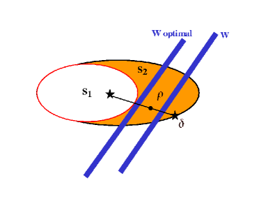
Figure 3: Schematic representation of a witness operator and an optimal witness operator.

To this aim one introduces the notion of a witness being finer than another one opti . A witness $W_{2}$ is called finer than $W_{1}$, if every operator that is detected by $W_{1}$ is also detected by $W_{2}$. A witness $W$ is optimal if there does not exist a witness that is finer than $W$. Let us denote by $P_{1}$ the set of operators $Z_{1}$ such that for every $\varrho_{1}\in S_{1}$, ${\rm Tr}(Z_{1}\varrho_{1})\geq 0$. The set $P_{1}$ is convex and for most of the applications that we consider compact. It contains witness operators and the so-called pre-witness operators, that have positive trace with the operators from $S_{1}$ but do not detect anything. Similarly, we define the set $P_{2}$ of operators $Z_{2}$ such that for every $\varrho\in S_{2}$, ${\rm Tr}(Z_{2}\varrho_{2})\geq 0$. The set $P_{2}$ is also convex and (in most applications) compact, and contained in $P_{1}$. We have the following theorems:
Theorem 2. If a witness $W_{2}$ is finer than $W_{1}$, then $W_{1}=(1-\epsilon)W_{2}+\epsilon Z_{2}$, where $Z_{2}\in P_{2}$.
The proof is a straightforward generalization of the proof of Lemma 2 from Ref. opti . Similarly, we obtain the generalization of Theorem 1 in Ref. opti (see also hulpke ):
Theorem 2’. A witness $W$ is optimal iff for all $Z_{2}\in P_{2}$ and $\epsilon>0$, $W^{\prime}=(1-\epsilon)W-\epsilon Z_{2}$ is not a witness, i.e. it does not fulfill ${\rm Tr}(Z_{1}\varrho_{1})\geq 0$ for all $Z_{1}$ from $P_{1}$.
¿From the above Theorem 2’ we see that optimal witnesses can be regarded as edge states (pertaining to the pair $P_{2}\subset P_{1}$); we will call them edge witnesses. We have a straightforward generalization of Theorem 1:
Theorem 3. Every witness $W\in P_{1}$ can be decomposed as a convex combination of an operator $Z_{2}\in P_{2}$ and an optimized witness $W_{opt}\in P_{1}\setminus P_{2}$,

$$W=\Lambda Z_{2}+(1-\Lambda)W_{opt},$$ (3)

where $1\geq\Lambda\geq 0$. The above decomposition is optimal in the sense that $W_{opt}$ can only have a trivial decomposition with the corresponding $\Lambda=0$. There exists the best decomposition, for which $\Lambda$ is maximal and unique.

Note that, as above, the optimal decomposition is not unique, and that when $\Lambda=1$ then $W\in P_{2}$ and $W$ ceases to be a witness, since it does not detect anything. Note also that optimal decompositions can be obtained in a constructive way, by subtracting operators $Z_{2}\in P_{2}$ from $W$, keeping the remainder in $P_{1}$. It is sufficient to subtract $Z_{2}\in P_{2}$ that are extremal points of the convex set $P_{2}$.

Finally, note that optimal witnesses (i.e. edge witnesses) characterize fully the witness operators that belong to $P_{1}\setminus P_{2}$, and every extremal point of the convex set $P_{1}$ is either an element of $P_{2}$, or an edge witness. The construction of examples of edge witnesses is possible by constructing optimal decompositions.

III.5 Canonical form of witnesses and linear maps

It is relatively easy to formulate the generalization of the theorems that were proven in Ref. char . In particular, we have the following theorem about the canonical form of the witness operators. Let $\hat{\mbox{$1{\bf l}$}}=\mbox{$1{\bf l}$}/{\rm Tr}\mbox{$1{\bf l}$}$, then we have:
Theorem 4. Every witness operator has the canonical form

$$W=(1+\epsilon)Z_{2}-\epsilon\hat{\mbox{$1{\bf l}$}},$$ (4)

where $Z_{2}\in P_{2}$, and there exists an edge operator $\delta$ such that ${\rm Tr}(Z_{2}\delta)=0$. The parameter $\epsilon$ fulfills

$$\epsilon/(1+\epsilon)\leq\inf_{\varrho_{1}\in S_{1}}{\rm Tr}(Z_{2}\varrho_{1}).$$ (5)

The proof that $\epsilon>0$ is the following. We consider the family $W+\tilde{\epsilon}\hat{\mbox{$1{\bf l}$}}$ for increasing $\tilde{\epsilon}$. For some finite range of $\tilde{\epsilon}$’s, $0\leq\tilde{\epsilon}\leq\epsilon_{0}$, this family consists of witnesses (which are positive on all elements of $S_{1}$, and are non–positive on at least one element of $S_{2}$). Let us consider $\epsilon_{0}$ for which ${\rm Tr}(W+\epsilon_{0}\hat{\mbox{$1{\bf l}$}})\varrho$ is non-negative for all $\varrho\in S_{2}$. From compactness of $S_{2}$ there exists a $\varrho_{0}$ such that ${\rm Tr}(W+\epsilon_{0}\hat{\mbox{$1{\bf l}$}})\varrho_{0}=0$. There cannot exist an optimal decomposition of $\varrho_{0}=\Lambda\varrho_{1}+(1-\Lambda)\delta$ with $\Lambda\neq 0$, since otherwise ${\rm Tr}(W+\tilde{\epsilon}\hat{\mbox{$1{\bf l}$}})\varrho_{1}$ would be negative for $\tilde{\epsilon}<\epsilon_{0}$, ergo $\varrho_{0}=\delta$ is an edge operator. From this argument it follows immediately that $(1+\epsilon_{0})Z_{2}=W+\epsilon_{0}\hat{\mbox{$1{\bf l}$}}$, and thus that ${\rm Tr}(Z_{2}\varrho_{1})$ is strictly positive for all $\varrho_{1}\in S_{1}$. Due to compactness the same has to hold for the infimum of this quantity.

There exists an elegant isomorphism jami between operators and linear maps, which allows to construct maps that “detect” states that do not belong to $S_{1}$. We will consider here the isomorphism for two-party systems, but it can be generalized and is in fact quite useful to study many-party systems homanypar .

Let an operator $O_{BC}\in{\cal B}(H_{B}\otimes H_{C})$. Then we can define a map

$$E:\ {\cal B}(H_{B})\to{\cal B}(H_{C}),$$ (6)

such that for any $\varrho_{B}\in{\cal B}(H_{B})$, we have

$$E(\varrho_{B})={\rm Tr}_{B}(O_{BC}\varrho_{B}^{T_{B}})\in{\cal B}(H_{C}),$$ (7)

where the trace is taken over the space $H_{B}$ only, and $T_{B}$ denotes the transposition in the space $H_{B}$.

Note that if we denote by $H_{B^{\prime}}$ a space isomorphic to $H_{B}$, we then have

$$\mbox{$1{\bf l}$}_{B^{\prime}}\otimes E(|\Psi\rangle\langle\Psi|)=O_{B^{\prime}C},$$ (8)

where

$$|\Psi\rangle=\sum_{i=1}^{{\rm dim}H_{B}}|i\rangle_{B^{\prime}}|i\rangle_{B}/\sqrt{{\rm dim}H_{B}}$$ (9)

is the maximally entangled state. Note that if $O_{B^{\prime}C}$ is a witness that detects $\varrho_{B^{\prime}C}$ (i.e. if ${\rm Tr}_{B^{\prime}C}(O_{B^{\prime}C}\varrho_{B^{\prime}C})<0$), then the adjoint map

$$\mbox{$1{\bf l}$}_{B^{\prime}}\otimes E^{{\dagger}}(\varrho_{B^{\prime}C})={\rm Tr}_{C}(O_{BC}^{T_{B}}\varrho_{B^{\prime}C})=\varrho_{B^{\prime}B}\in{\cal B}(H_{B^{\prime}}\otimes H_{B})$$ (10)

transforms $\varrho_{B^{\prime}C}$ into an operator $\varrho_{B^{\prime}B}$ which is not positive definite, and ${\rm Tr}_{B^{\prime}B}(\varrho_{B^{\prime}B}|\Psi\rangle\langle\Psi|)<0$. If the adjoint map acting on some $\varrho$ produces a non-positive operator, we say that it detects $\varrho$. Maps detect more operators than witnesses. For instance, if the map detects $\varrho_{B^{\prime}C}$, then it also detects $O_{B^{\prime}}\varrho_{B^{\prime}C}O_{B^{\prime}}^{{\dagger}}$ for any $O_{B^{\prime}}$, where $O_{B^{\prime}}$ is an element of the linear group $GL(H_{B^{\prime}})$.

If the operator $O_{BC}$ has some properties, then it implies some properties of the corresponding map $E[O_{BC}]$. For instance, if $O_{BC}$ is positive definite, then $E[O_{BC}]$ is a completely positive map (CPM), if $O_{BC}$ is an entanglement witness, then $E[O_{BC}]$ is positive (PM), if $O_{BC}$ is a decomposable entanglement witness, i.e. $O_{BC}=P+Q^{T_{B}}$, where both $P,Q\in{\cal B}(H_{B}\otimes H_{C})$ are positive, then $E[O_{BC}]$ is a decomposable positive map, i.e. a convex sum of a CPM and another CPM composed with the partial transposition in $H_{B}$. Similarly, if $O_{BC}$ is a non–decomposable entanglement witness, i.e. $O_{BC}$ cannot be represented as $P+Q^{T_{B}}$, where both $P,Q\in{\cal B}(H_{B}\otimes H_{C})$ are positive, then $E[O_{BC}]$ is a non–decomposable positive map. Schmidt number witnesses adm are related to the so-called $k$–positive maps barpaw .

In all of the above mentioned examples, the maps have some positivity properties on the operators from the corresponding set $S_{1}$ (separable state, PPT states, states of Schmidt number $k$ etc). It is not clear if that will always be the case, if one considers a general abstract formulation of the problem. Quite generally, however, we can say that if $W_{BC}$ is a witness, i.e. ${\rm Tr}(W_{BC}\sigma_{BC})\geq 0$ for every $\sigma_{BC}$ from $S_{1}$, then the corresponding adjoint map

$$\mbox{$1{\bf l}$}_{B^{\prime}}\otimes E^{{\dagger}}(\sigma_{B^{\prime}C})={\rm Tr}_{C}(W_{BC}^{T_{B}}\sigma_{B^{\prime}C})=\sigma_{B^{\prime}B}$$ (11)

has the property that $\langle\Psi|\sigma_{B^{\prime}B}|\Psi\rangle\geq 0$.

The analysis of the maps completes our presentation of the I–Ha programme. Note that the knowledge of the canonical form of witnesses allows to construct the canonical form of the corresponding maps.

IV IV. Applications of the I–Ha Programme

In this section we will discuss in more detail the application of the I-Ha programme to concrete problems: the separability problem, the relation between optimal separability witnesses and non-distillable NPPT states, the Schmidt number of mixed states, and finally the classification of mixed states of three-qubit systems.

Before turning to a more detailed discussion let us list the results and applications of the I-Ha programme achieved so far:

• The optimal decomposition in the context of separability (optimal separable approximations and best separable approximations, BSA) have been introduced in Ref. M&A . The theory of optimal decompositions, and in particular of optimal decompositions of PPT states is presented in karnas . Important results concerning the best separable approximations for $2\otimes 2$ systems have been obtained by B.-G. Englert englert . An analytic construction of the BSA in this case was recently achieved by Kuś and Wellens kus .

• The construction of “edge” states and the solution of the separability problem for low rank states were discussed by us in Refs. pra1 ; pra2 ; pra3 for $2\otimes N$, $M\otimes N$ and $2\otimes 2\otimes N$ systems, respectively.

• The canonical form of witnesses and positive maps and their optimization is discussed in Refs. char ; opti ; adm .

• The I–Ha programme has also been applied to study quantum correlations in fermionic systems fermi , Schmidt number witnesses adm , and three-qubit systems abls .

• The programme is presented partially in the primer primer and in the tutorial tutor .

• The programme has been also applied to study systems with continuous variables (CV). We have provided the first example of PPT states for CV systems pptcv , and solved the separability problem for two-party Gaussian states with an arbitrary number of modes gauss1 , and for three-party systems each having a single mode gauss2 . Werner and Wolf werwol used the I-Ha approach to provide first examples of the Gaussian PPT states – “edge” states in our terminology.

• The I-Ha programme was extended to study separability and entanglement of quantum operations oper .

We will now discuss some applications, and in particular we will show how they fit into the general scheme discussed in the previous section.

IV.1 Application I - the separability problem

Two kinds of applications were discussed by us in this context: the application to the general problem of separability, in which $S_{1}$ is the set of separable states $S$, whereas $S_{2}$ is the set of all states, denoted here as $B$ M&A ; karnas ; opti . Another application concerns the problem of distinguishing separable states from PPT entangled states: in this case $S_{1}=S$, whereas $S_{2}$ is the set of PPT states, so that the set of PPTES’s is given by $PPT\setminus S_{1}$. For the first application we have:

Proposition 1.M&A Every state $\rho\in{\cal B}(H_{A}\otimes H_{B})$ can be decomposed as

$$\varrho=\Lambda\sigma+(1-\Lambda)\delta,$$ (12)

where $\sigma\in S$, and $\delta$ is an edge state, which in this situation means a state whose range $R(\delta)$ does not contain any product vector $|e,f\rangle$.

Similarly, for the second scenario we have:

Proposition 2.pra1 ; karnas Every state $\varrho\in{\cal B}(H_{A}\otimes H_{B})$ having the PPT property can be decomposed as

$$\varrho=\Lambda\sigma+(1-\Lambda)\delta,$$ (13)

where $\sigma\in S$, and $\delta$ is a PPT edge state, which in this situation means a state whose range $R(\delta)$ does not contain any product vector $|e,f\rangle$, such that the range of the partially transposed state $R(\delta^{T_{A}})$ contains at the same time the partially complex conjugated vector $|e^{*},f\rangle$.

Note that a similar proposition can be proven for the case when $S_{1}=PPT$ and $S_{2}=B$. Such an optimal decomposition is difficult to realise in a constructive way, since the subtraction of a projector onto a product vector must be replaced in this case by the subtraction of a PPT state $\sigma$ whose range fulfills at the same time $R(\sigma)\subset R(\delta)$, $R(\sigma^{T_{A}})\subset R(\delta^{T_{A}})$.

Let us denote by $r(\varrho)$ the rank of $\varrho$. The studies of PPT edge states has led us to the following proposition (pra1 ; pra2 , see pra3 for the generalization to $2\otimes 2\otimes N$ systems):

Proposition 3. If a state $\varrho$ acting in an $M\otimes N$ dimensional Hilbert space fulfills that

$$r(\varrho)+r(\varrho^{T_{A}})\leq 2MN-M-N+2$$ (14)

then there exists generically a finite number of product states that belong to $R(\delta)$, such that the range of the partially transposed state $R(\delta^{T_{A}})$ contains at the same time the partially complex conjugated vector $|e^{*},f\rangle$.

Note that in such a case it is easy to check if $\varrho$ is separable, since we know the finite number of projectors onto product vectors that can enter the decomposition of $\varrho$ into a convex sum of projectors on product vectors. This means that for $r(\varrho)+r(\varrho^{T_{A}})\leq 2MN-M-N+2$ the separability problem is essentially solved.

It is useful to quote at this point the propositions that provide the explicit form of entanglement witnesses (EW) for edge states and canonical forms of witnesses for the two cases introduced above, $S_{2}=B$ and $S_{2}=PPT$:

Proposition 4. Given an edge state $\delta$,

$$W=P-\epsilon\mbox{$1{\bf l}$},$$ (15)

where $P\geq 0$, $R(P)=K(\delta)$, and

$$\epsilon\leq\inf_{|e,f\rangle}\langle e,f|P|e,f\rangle$$

is a decomposable EW that detects $\delta$.

Proposition 4’. Given a PPT edge state $\delta$,

$$W=P+Q^{T_{A}}-\epsilon\mbox{$1{\bf l}$},$$ (16)

where $P\geq 0$, $R(P)=K(\delta)$, $Q\geq 0$, $R(Q)=K(\delta^{T_{A}})$, and

$$\epsilon\leq\inf_{|e,f\rangle}\langle e,f|P+Q^{T_{A}}|e,f\rangle$$

is a non-decomposable EW (nd-EW) that detects $\delta$.

Conversely,

Proposition 5. If $W$ is a decomposable EW then there exists an edge state $\delta$ such that

$$W=P-\epsilon\mbox{$1{\bf l}$},$$ (17)

where $P\geq 0$, $R(P)=K(\delta)$, and

$$\epsilon\leq\inf_{|e,f\rangle}\langle e,f|P|e,f\rangle.$$

Proposition 5’. If $W$ is a non-decomposable EW, then there exists a PPT edge state $\delta$ such that

$$W=P+Q^{T_{A}}-\epsilon\mbox{$1{\bf l}$},$$ (18)

where $P\geq 0$, $R(P)=K(\delta)$, $Q\geq 0$, $R(Q)=K(\delta^{T_{A}})$, and

$$\epsilon\leq\inf_{|e,f\rangle}\langle e,f|P+Q^{T_{A}}|e,f\rangle.$$

Note that proposition 4(4’) and 5(5’) together with the optimization allow to formulate necessary conditions for witness operators to be extremal in the convex set of all witnesses. The Jamiołkowski isomorphism translates those conditions into necessary conditions for positive maps to be extremal char .

The two kinds of optimization (related to pairs of sets $S,B$ and $S,PPT$) are schematically illustrated in Fig. 4. It is perhaps easier to understand them when one looks at Fig. 5. Here we see that the set of $pre-EW$ of decomposable EW together with B is convex and compact (this is a set of operators $W$ that fulfill the condition ${\rm Tr}(W\sigma)\geq 0$ for all $\sigma\in PPT$). Similarly, adding the set of non-decomposable witnesses to this set, one obtains yet another convex and compact set of $pre-nd-EW$ which contains operators $W$ such that ${\rm Tr}(W\sigma)\geq 0$ for all $\sigma\in S$.

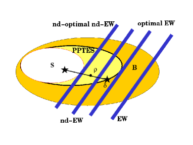
Figure 4: Schematic representation of a decomposable witness operator, an optimal decomposable witness operator, a non–decomposable witness operator, and optimal non–decomposable witness operator (see hyperplanes from right to left).

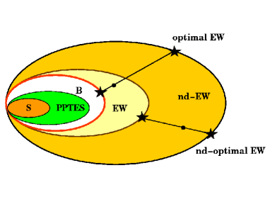
Figure 5: Schematic representation of the optimization of decomposable or non–decomposable entanglement witnesses as search for optimal decompositions and decomposable, or non-decomposable “edge” witnesses.

Figure 5 allows us immediately to write for the case $S_{1}=B$ and $S_{2}=pre-EW$:
Proposition 6. Every $EW\in pre-EW$ can be decomposed as a convex combination of an operator $\varrho\in B$ and $\delta\in pre-EW\setminus B$,

$$EW=\Lambda\varrho+(1-\Lambda)\delta,$$ (19)

where $1\geq\Lambda\geq 0$. In the above decomposition $\delta$ is an optimal entanglement witness in the sense that $\delta$ can only have a trivial decomposition with the corresponding $\Lambda=0$. There exists the best decomposition, for which $\Lambda$ is maximal and unique.
Similarly, for non-decomposable EW’s we have:
Proposition 7. Every $nd-EW\in pre-EW$ can be decomposed as a convex combination of an operator $\varrho\in pre-EW$ and $\delta\in pre-nd-EW\setminus pre-EW$,

$$EW=\Lambda\varrho+(1-\Lambda)\delta,$$ (20)

where $1\geq\Lambda\geq 0$. In the above decomposition $\delta$ is an optimal nd-entanglement witness in the sense that $\delta$ can only have a trivial decomposition with the corresponding $\Lambda=0$. There exists the best decomposition, for which $\Lambda$ is maximal and unique.
The proofs are the same as in the original works (c.f. M&A ; pra1 ; karnas ).

IV.2 Application II – Optimal witnesses and non-distillable NPPT states

Let us first remind the readers that it has been recently conjectured npt1 ; npt2 that there exist states with non-positive partial transpose that are non-distillable. In particular, in Ref. npt1 we have formulated the following Conjecture. Let $\dim H_{A}=\dim H_{B}=d$, and let

$$\varrho_{W}(\beta)=\frac{1}{N_{W}}(\mbox{$\cal P$}_{s}+\alpha(\beta)\mbox{$\cal P$}_{a}),$$

$$\varrho_{W}^{T_{A}}(\beta)=\frac{1}{\tilde{N}_{W}}(\mbox{$1{\bf l}$}-\beta\mbox{$\cal P$}),$$ (21)

where $\mbox{$\cal P$}_{s,a}$ are the projectors onto the symmetric respectively antisymmetric subspace, $\cal P$ is the projector onto a maximally entangled vector $|\Psi\rangle=\sum_{i=1}^{d}|i\rangle_{A}|i\rangle_{B}/\sqrt{d}$, $\alpha(\beta)=\frac{d+\beta}{d-\beta}$ and $N_{W},\tilde{N}_{W}$ are normalization constants. Then, $\varrho_{W}(\beta)$ is a non-distillable NPPT state for $\beta\in(1,d/2]$.

Note that for $-1\leq\beta<1$, $\varrho_{W}(\beta)$ is PPT (it is in fact separable). The above conjecture is supported by numerical evidence for 2 and 3 copies of $\varrho_{W}(\beta)$, and the fact that $\varrho_{W}(\beta)$ is $n$-copy non-distillable for $1<\beta\leq\beta_{n}$. The later statement means, that in this case one cannot project $n$ copies of $\varrho_{W}(\beta)$ onto a $2\otimes 2$-dimensional subspace of $H_{A}^{\otimes n}\otimes H_{B}^{\otimes n}$, such that the resulting $2\otimes 2$ state would be distillable, i.e. would not have the PPT property. The best bounds on $\beta_{n}$ are $\beta_{1}=d/2$, $\beta_{2}=(2+d)/4$, etc. Unfortunately $\beta_{n}\to 1$, when $n\to\infty$.
It is interesting to observe that the existence of $n$-copy non-distillable NPPT states allows the construction of optimal EW’s. To this aim we present the following:
Proposition 8 Let $\dim H_{A^{\prime}}=\dim H_{B^{\prime}}=2$, and let $\mbox{$\cal P$}_{a}$ be the projector onto the singlet state $(|0\rangle_{A^{\prime}}|1\rangle_{B^{\prime}}-|1\rangle_{A^{\prime}}|0\rangle_{B^{\prime}})/\sqrt{2}$ in $H_{A^{\prime}}\otimes H_{B^{\prime}}$. Let $W(\beta)$ act on $(H_{A^{\prime}}\otimes H_{A}^{\otimes n})\otimes(H_{B^{\prime}}\otimes H_{B}^{\otimes n})$, where

$$W(\beta)=\mbox{$\cal P$}_{a}^{T_{A^{\prime}}}\otimes(\varrho_{W}(\beta))^{\otimes n}.$$ (22)

Then we have:

i)

$W(\beta)$ is an optimal non-decomposable EW for $0<\beta\leq\beta_{n}$.

ii)

$W(\beta)$ is an nd-optimal non-decomposable EW for $n=1$, $\beta=d/2$.

Additionally, if the conjecture is true we have:
Proposition 9 If the conjecture is true, the $W(\beta)$ defined in proposition 8 is

i)

an optimal non-decomposable EW for $\beta\in(1,d/2]$.

ii)

an nd-optimal non-decomposable EW for $\beta=d/2$.

In the above propositions “optimal EW” means optimal with respect to subtraction of positive operators ($S_{1}=B,S_{2}=\mbox{pre-EW}$). The proof of proposition 8 follows directly from the results of Ref. opti .

It is easy to see that if $|e,f\rangle$ is a product vector from $(H_{A^{\prime}}\otimes H_{A}^{\otimes n})\otimes(H_{B^{\prime}}\otimes H_{B}^{\otimes n})$, then $\langle e,f|W(\beta)|e,f\rangle\geq 0$, provided $\langle\Psi_{2}|(\varrho_{W}^{T_{A}}(\beta))^{\otimes n}|\Psi_{2}\rangle\geq 0$ for all $|\Psi_{2}\rangle\in H_{A}^{\otimes n}\otimes H_{B}^{\otimes n}$ of Schmidt rank 2. On the other hand $W(\beta)$ is not positive, so it detects some states, i.e. $W(\beta)$ is an EW. Moreover, $\langle e,f|W(\beta)|e,f\rangle=0$ for all $|e\rangle=|E\rangle|F\rangle_{A}$, $|f\rangle=|E^{*}\rangle|G\rangle_{B}$. Since such vectors span the whole Hilbert space, $W(\beta)$ is an optimal EW. From Ref. opti we know, however, that an optimal decomposable EW must be of the form

$$W(\beta)=Q^{T_{A}},\mbox{ where }Q\geq 0.$$ (23)

This is not the case, ergo $W(\beta)$ is an optimal non-decomposable EW for $0\leq\beta\leq\beta_{n}$, which proves part (i) of the proposition. Proving part (ii) is achieved by observing that for $\beta=d/2$ there exists another set of product vectors $|\tilde{e},\tilde{f}\rangle$ such that $\langle\tilde{e},\tilde{f}|W^{T_{A}}(\frac{d}{2})|\tilde{e},\tilde{f}\rangle=0$, and $|\tilde{e},\tilde{f}\rangle$ span the whole Hilbert space. The vectors $|\tilde{e},\tilde{f}\rangle$ are such that

$${\rm Tr}_{A^{\prime}B^{\prime}}(\mbox{$\cal P$}_{a}|\tilde{e},\tilde{f}\rangle\langle\tilde{e},\tilde{f}|)=|\psi_{2}\rangle\langle\psi_{2}|\ ,$$ (24)

where $|\psi_{2}\rangle$ are vectors of Schmidt rank 2 in $H_{A}\otimes H_{B}$ such that

$$\langle\psi_{2}|\varrho_{W}^{T_{A}}\left(\frac{d}{2}\right)|\psi_{2}\rangle=0.$$ (25)

Quite generally $|\psi_{2}\rangle=\frac{1}{\sqrt{2}}(|e,e^{*}\rangle+|e_{\perp},e_{\perp}^{*}\rangle)$ where $|e\rangle$ is an arbitrary vector from $H_{A}$, and $|e_{\perp}\rangle$ is an arbitrary vector from $H_{A}$ orthogonal to $|e\rangle$. The proof of proposition 9 is analogous.
Note that propositions 8 and 9 do not involve a specific form of $\varrho_{W}(\beta)$, and are valid for all NPPT non-distillable states. Note also, that proposition 8 implies immediately the recent result in pptdist , that 1-copy non-distillable NPPT states are PPT-distillable. To this aim we observe that if $W(\beta)$ is already non-decomposable for $n=1$, then it detects some PPT state $\sigma$, i.e.

$${\rm Tr}(W(\beta)\sigma)<0\ ,$$ (26)

that implies that

$${\rm Tr}_{AA^{\prime}BB^{\prime}}(\sigma^{T_{A^{\prime}A}}[\mbox{$\cal P$}_{a}\otimes\varrho_{W}^{T_{A}}(\beta)])<0\ ,$$ (27)

which in turn allows to define a linear PPT map $E_{W(\beta)}(\varrho)={\rm Tr}_{AB}(\sigma^{T_{A}}\varrho^{T_{A}})={\rm Tr}_{AB}(\sigma\varrho)=\tilde{\varrho}$ which transforms $\varrho$ into a matrix $\tilde{\varrho}$ in dimension $2\otimes 2$ which is NPPT, since ${\rm Tr}(\tilde{\varrho}^{T_{A^{\prime}}}\mbox{$\cal P$}_{a})<0$.

In barbara we develop a general formalism which connects entanglement witnesses to the distillation and activation properties of a state. There we also show its applications to three-party states and point out how it can be generalized to an arbitrary number of parties.

IV.3 Application III – Schmidt number of mixed states

The I-Ha programme can be applied to detect how many degrees of freedom of a given bipartite state are entangled – this is the interpretation of the so-called Schmidt number of a mixed state. The Schmidt number is a generalization of the Schmidt rank of pure bipartite states and was introduced in barpaw (more implicitly defined in Vidal ): a given state $\varrho$ can be expanded as

$$\varrho=\sum_{i}p_{i}|\,\psi_{i}^{r_{i}}\rangle\langle\psi_{i}^{r_{i}}\,|\ ,$$ (28)

with $p_{i}\geq 0$ and $\sum_{i}p_{i}=1$. Here $r_{i}$ denotes the Schmidt rank of the pure state $|\,\psi_{i}\rangle$. The maximal Schmidt rank in this decomposition is called $r_{\rm max}$. The Schmidt number $k$ of $\varrho$ is given as the minimum of $r_{\rm max}$ over all decompositions,

$$k=\mbox{ min}\{r_{\rm max}\}\ .$$ (29)

Namely, $k$ tells us how many degrees of freedom have at least to be entangled in order to create $\varrho$. This number cannot be greater than $M$, the smaller dimension of the two subsystems.

With this definition one realises that the set of all states consists of compact convex subsets of states that carry the same Schmidt number. We denote the subset that contains states of Schmidt number $k$ or less by $S_{k}$. These Schmidt classes are successively embedded into each other, $S_{1}\subset S_{2}\subset...\subset S_{M}$. This is illustrated in Figure 6.

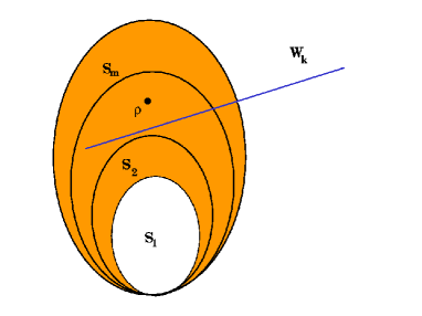
Figure 6: Schematic representation of Schmidt classes and their detection by Schmidt witnesses.

In adm we generalized the concept of entanglement witnesses to Schmidt number witnesses. The generalization is straightforward:
Definition 3. An operator $W_{k}$ is a witness operator of Schmidt number $k$ iff for every $\sigma\in S_{k-1}$ it holds that ${\rm Tr}(\sigma W_{k})\geq 0$, and there exists a $\varrho\in S_{k}$ for which ${\rm Tr}(\varrho W_{k})<0$. We say that $W_{k}$ detects $\varrho$. We normalize the witnesses demanding that ${\rm Tr}(W_{k})=1$.

Applying the I-Ha programme to Schmidt classes, we can write a state $\varrho$ as a convex combination of a state from Schmidt class $k$ and an edge state,

$$\varrho=\Lambda\varrho_{k}+(1-\Lambda)\delta\ ,$$ (30)

where the edge state $\delta$ has no vectors of Schmidt rank $\leq k$ in its range. This decomposition can be obtained by subtracting projectors onto vectors of Schmidt rank $\leq k$ from $\varrho$, while requiring the resulting state to be positive.

A canonical form for a witness of the Schmidt class $k$ is given by

$$W_{k}=Q-\epsilon\mbox{$1{\bf l}$}\ ,$$ (31)

where $Q$ is a positive operator that fulfills $K(Q)=R(\delta)$, for some edge state $\delta$ with Schmidt number $k$. We define $\epsilon\equiv\mbox{ inf}_{|\,\psi\rangle}\langle\psi\,|Q|\,\psi\rangle$, where $|\,\psi\rangle$ has Schmidt rank $\leq k-1$. This construction guarantees that the requirements from Definition 3 are met: the parameter $\epsilon$ is chosen such that ${\rm Tr}(\sigma W_{k})\geq 0$ holds for every $\sigma\in S_{k-1}$, and $\delta$ is detected by $W_{k}$.

The optimization of Schmidt witnesses can be performed in an analogous way as for entanglement witnesses and is discussed in adm ; hulpke . An example of an optimal (unnormalized) witness of Schmidt number $k$ in $H^{M}\otimes H^{M}$ is given by

$$W_{k,opt}=\mbox{$1{\bf l}$}-\frac{M}{k-1}\mbox{$\cal P$}\ ,$$ (32)

where $\cal P$ is the projector onto the maximally entangled state $|\Psi\rangle=\sum_{i=1}^{M}|\,ii\rangle/\sqrt{M}$. The fact that the maximal squared overlap between $|\Psi\rangle$ and a vector with Schmidt rank $k$ is $k/M$ leads to the correct properties for a $k$-Schmidt witness.

IV.4 Application IV – Mixed three-qubit states

Recently studies of tripartite states have been incorporated in the I-Ha programme abls : composite systems of three qubits can be classified according to Figure 7. This figure should be regarded as an intuitive picture of the structure of this set.

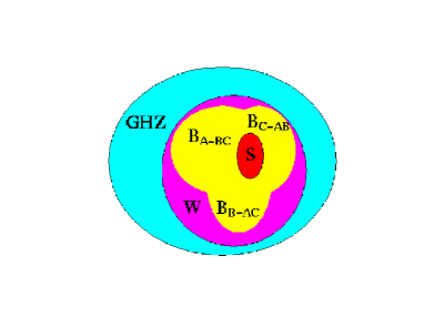
Figure 7: Classification of mixed three-qubit states.

The class $S$ denotes separable states, i.e. states that can be written as a convex combination of product states of the three parties. The class $B$ stands for biseparable states, i.e. those that have vectors in their decomposition in which two out of the three parties are entangled, and the third one is in a product state with the two entangled ones. There are three possibilities for such biseparable states, which are indicated as three petals in the figure. The biseparable class is understood to be the convex hull of them. The biseparable states are embedded in the $W$-class. This is the set of states that also have vectors of the form

$$|\,\psi_{W}\rangle=\mbox{$\textstyle\frac{1}{\sqrt{3}}$}(|\,100\rangle+|\,010\rangle+|\,001\rangle)\$$ (33)

in their decomposition. These so-called W-vectors were introduced in duer , and shown to be locally inequivalent to the GHZ-vectors, which are of the form

$$|\,\psi_{GHZ}\rangle=\mbox{$\textstyle\frac{1}{\sqrt{2}}$}(|\,000\rangle+|\,111\rangle)\ .$$ (34)

In Figure 7 the GHZ-class, i.e. the set of states that have GHZ-vectors in their decomposition, surrounds the W-states. This is the correct ordering of states, as each of the inner sets is required to be compact. By studying the most general form of a W-state and a GHZ-state, as given in tony , one realizes that swapping the role of the classes GHZ and W would lead to a GHZ-class that is not compact. The reason is that infinitesimally close to any W-state there always lies a GHZ-state.

Again, one can construct witnesses to detect the class of a given mixed three-qubit state. We called them biseparable witnesses, W-witnesses and GHZ-witnesses. Their definition is a straightforward extension of Definition 3. Using an explicit W-witness, e.g.

$$W_{W}=\mbox{$\textstyle\frac{1}{2}$}\mbox{$1{\bf l}$}-\mbox{$\cal P$}_{GHZ}\ ,$$ (35)

where $\mbox{$\cal P$}_{GHZ}$ is a projector onto a GHZ-vector, we showed in abls that the set of $W\setminus B$ is not of measure zero, contrary to the pure case duer . The idea is to take a state from the family

$$\varrho=\frac{1-p}{8}\mbox{$1{\bf l}$}+p\mbox{$\cal P$}_{W}\ ,$$ (36)

where $\mbox{$\cal P$}_{W}$ is the projector onto a pure W-state, and show that for certain values of the parameter $p$ a ball of states surrounding $\varrho$ is in $W\setminus B$. This ball is given by $\tilde{\varrho}=(1-\kappa)\varrho+\kappa\sigma$, where $\sigma$ is arbitrary, and the task was to show that there is a finite range of $\kappa$ such that $\tilde{\varrho}$ is still contained in $W\setminus B$.

Another topic that we have studied in the I-Ha programme is the question whether bound entangled states can be found in any of the described entangled sets abls ? Our conjecture is that this is not the case, and that bound entangled states cannot be in $GHZ\setminus W$.

For small ranks, namely $r(\varrho)\leq 4$, it is clear that bound entangled states even have to be biseparable, i.e. can be neither in $W\setminus B$ nor in $GHZ\setminus W$: viewing $\varrho$ as a state from the Hilbert space of $2\otimes 4$ type we can use the result from pra1 that any $2\otimes 4$ PPT state with rank $\leq 4$ is separable.

For higher ranks, the idea leading to our conjecture is as follows: bound entangled states can only be detected by non-decomposable witnesses, i.e. operators of the form

$$W_{nd} = W_{d}-\epsilon\mbox{$1{\bf l}$}\ ,$$

$$W_{d} = P+\sum_{X}Q^{T_{X}}_{X}\ ,$$ (37)

with $P,Q_{X}\geq 0$, $R(P)=K(\varrho)$, $R(Q_{X})=K(\varrho^{T_{X}})$, where $X=A,B,C$. We need to show that it is always possible to find a W–state $|\,\phi_{W}\rangle$ with $\langle\phi_{W}\,|W_{d}|\,\phi_{W}\rangle\leq 0$, and therefore $\langle\phi_{W}\,|W_{nd}|\,\phi_{W}\rangle<0$. If this is the case, then $W_{nd}$ cannot be a GHZ–witness, and thus $\varrho$ belongs to the $W$–class.

In trying to find $|\,\phi_{W}\rangle$ we compared the number of free parameters with the number of equations to solve, which depend on the rank of $\varrho$. It turns out that there is much freedom, and it is very likely to find such $|\,\phi_{W}\rangle$. We therefore have some evidence for $\varrho_{BE}\not\in GHZ\setminus W$.

V V. Summary

We have shown that, although the separability problem and the problem of characterization and classification of positive maps is not yet solved, enormous progress has been achieved in the last years. Nevertheless, in spite of being more than 100 years old, quantum theory is still extraordinary challenging.

VI VI. Acknowledgements

We wish to thank A. Acín, H. Briegel, W. Dür, K. Eckert, J. Eisert, A. Ekert, G. Giedke, M. Horodecki, R. Horodecki, S. Karnas, M. Kuś, D. Loss, C. Macchiavello, A. Pittenger, M. Plenio, J. Samsonowicz, J. Schliemann, R. Tarrach, F. Verstraete and G. Vidal for discussions in the context of the I-Ha programme and at the Gdansk meeting. This work has been supported by the DFG (SFB 407 and Schwerpunkt “Quanteninformationsverarbeitung”), and the ESF PESC Programme on Quantum Information.

References

- (1) E. Schrödinger, Naturwissenschaften 23, 807 (1935).
- (2) A. Einstein, B. Podolsky and N. Rosen, Phys. Rev. 47, 777 (1935).
- (3) “Quantum Theory and Measurement”, eds. J. Wheeler and W. Zurek, (Princeton Univ. Press, Princeton, NJ, USA, 1983).
- (4) “Quantum Theory: Concepts and Methods, A. Peres, (Kluwer Academic Publishers, The Netherlands, 1995).
- (5) The Physics of Quantum Information: Quantum Cryptography, Quantum Teleportation, Quantum Computation, eds. D. Bouwmeester, A. Ekert and A. Zeilinger, (Springer-Verlag, 2000); Quantum Computation and Quantum Information Theory, eds. C. Macchiavello, G. M. Palma and A. Zeilinger, (World Scientific, 2000); Quantum Computation and Quantum Information, M. Nielsen and I. Chuang, (Cambridge Univ. Press, 2000).
- (6) D. Bruß and N. Lütkenhaus, AAECC 10, 383 (2000); N. Gisin, G. Ribordy, W. Tittel and H. Zbinden, quant-ph/0101098.
- (7) C.H. Bennett, G. Brassard, S. Popescu, B. Schumacher, J.A. Smolin and W.K. Wootters, Phys. Rev. Lett. 76, 722 (1996).
- (8) E. Strømer, Acta. Math. 110, 233 (1963).
- (9) A. Jamiołkowski, Rep. Math. Phys. 3, 275 (1972).
- (10) M.-D. Choi, Linear Algebra Appl. 12, 95 (1975).
- (11) S.L. Woronowicz, Rep. Math. Phys. 10, 165 (1976).
- (12) G. Alber, T. Beth, M. Horodecki, P. Horodecki, R. Horodecki, M. Rötteler, H. Weinfurter, R.F. Werner and A. Zeilinger, “Quantum Information: An Introduction to Basic Theoretical Concepts and Experiments (Springer Tracts in Modern Physics, 173; Springer-Verlag, 2001).
- (13) B.M. Terhal, quant-ph/0101032.
- (14) M. Donald, M. Horodecki and O. Rudolph, quant-ph/0105017.
- (15) M. Lewenstein, D. Bruß, J.I. Cirac, B. Kraus, M. Kuś, J. Samsonowicz, A. Sanpera and R. Tarrach, J. Mod. Opt. 47, 2841 (2000).
- (16) D. Bruß, Proc. of the ICQI conference, Rochester (2001).
- (17) P. Horodecki, Proc. of the NATO ARW conference, Mykonos (2000).
- (18) B. Kraus, M. Lewenstein and J.I. Cirac, to be published.
- (19) R.F. Werner, Phys. Rev. A 40, 4277 (1989).
- (20) N. Gisin, Phys. Lett. A 145, 201 (1991); S. Popescu and D. Rohrlich, Phys. Lett. A 166, 293 (1992).
- (21) In the mathematical literature some versions of the properties pointed out in the context of separability were present even earlier in terms of cones of positive matrices (see especially posmaps1 ; posmaps3 , cf. jami ; posmaps2 ).
- (22) S. Popescu, Phys. Rev. Lett. 72, 797 (1994).
- (23) S. Popescu, Phys. Rev. Lett. 74, 2619 (1995).
- (24) N. Gisin, Phys. Lett. A 210, 151 (1996).
- (25) C.H. Bennett, G. Brassard, S. Popescu, B. Schumacher, J.A. Smolin and W.K. Wootters, Phys. Rev. Lett. 76, 722 (1996); C. H. Bennett, H. J. Bernstein, S. Popescu and B. Schumacher, Phys. Rev. A 53 2046 (1996); C.H. Bennett, D.P. DiVincenzo, J.A. Smolin and W.K. Wootters, Phys. Rev. A 54, 3825 (1997).
- (26) D. Deutsch, A. Ekert, R. Jozsa, C. Macchiavello, S. Popescu and A. Sanpera, Phys. Rev. Lett. 77, 2818 (1996).
- (27) A. Peres, Phys. Rev. Lett. 77, 1413 (1996).
- (28) M. Horodecki, P. Horodecki and R. Horodecki, Phys. Lett. A 223, 1 (1996).
- (29) P. Horodecki, Phys. Lett. A 232, 333 (1997).
- (30) M. Horodecki, P. Horodecki and R. Horodecki, Phys. Rev. Lett. 78, 574 (1997).
- (31) M. Horodecki, P. Horodecki and R. Horodecki, Phys. Rev. Lett. 80, 5239 (1998).
- (32) M. Horodecki, P. Horodecki and R. Horodecki, Phys. Rev. Lett. 82, 1046 (1999).
- (33) M. Horodecki and P. Horodecki, Phys. Rev. A 59, 4206 (1999).
- (34) M. Lewenstein and A. Sanpera, Phys. Rev. Lett. 80, 2261 (1998).
- (35) C. H. Bennett, D.P. DiVincenzo, T. Mor, P.W. Shor, J.A. Smolin and B.M. Terhal, Phys. Rev. Lett. 82, 5385 (1999).
- (36) B.M. Terhal, Phys. Lett. A 271, 319 (2000); B.M. Terhal, Linear Algebra Appl. 323, 61 (2000).
- (37) W. Dür, J.I. Cirac, M. Lewenstein and D. Bruß, Phys. Rev. A 61, 062313 (2000).
- (38) D.P. DiVincenzo, P.W. Shor, J.A Smolin, B.M. Terhal and A. Thapliyal, Phys. Rev. A 61, 062312 (2000).
- (39) S. Karnas and M. Lewenstein, J. Phys. A 34, 6919 (2001).
- (40) W. Rudin, “Functional Analysis”, (McGraw-Hill, New York, 1973).
- (41) P. Horodecki, M. Horodecki and R. Horodecki, J. Mod. Opt. 47, 347 (2000).
- (42) M. Lewenstein, B. Kraus, P. Horodecki and J.I. Cirac, Phys. Rev. A 63, 044304 (2001).
- (43) M. Lewenstein, B. Kraus, J.I. Cirac and P. Horodecki, Phys, Rev. A 62, 052310 (2000).
- (44) F. Hulpke, to be published.
- (45) M. Horodecki, P. Horodecki and R. Horodecki, Phys. Lett. A, 283, 1 (2001).
- (46) A. Sanpera, D. Bruß and M. Lewenstein, Phys. Rev. A 63, 050301(R) (2001).
- (47) B.M. Terhal and P. Horodecki, Phys. Rev. A 61, 040301(R) (2000).
- (48) G. Vidal, J. Mod. Opt. 47, 355 (2000).
- (49) B.-G. Englert and N. Metwally, quant-ph/9912089; B.-G. Englert and N. Metwally, quant-ph/0007053.
- (50) T. Wellens and M. Kuś, quant-ph/0104098, to be publ. in Phys. Rev. A.
- (51) B. Kraus, J.I. Cirac, S. Karnas and M. Lewenstein, Phys Rev. A 61, 062302 (2000).
- (52) P. Horodecki, M. Lewenstein, G. Vidal and J.I. Cirac, Phys. Rev. A 62, 032310 (2000).
- (53) S. Karnas and M. Lewenstein, Phys. Rev. A 64, 042313 (2001).
- (54) J. Schliemann, J.I. Cirac, M. Kuś, M. Lewenstein and D. Loss, Phys. Rev A 64, 022303 (2001).
- (55) A. Acín, D. Bruß, M. Lewenstein and A. Sanpera, Phys. Rev. Lett. 87, 040401 (2001).
- (56) P. Horodecki and M. Lewenstein, Phys. Rev. Lett. 85, 2657 (2000).
- (57) G. Giedke, B. Kraus, M. Lewenstein and J.I. Cirac, quant-ph/0104050, Phys. Rev. Lett., in print.
- (58) P. Horodecki and M. Lewenstein, quant-ph/0103076.
- (59) R.F. Werner and M.M. Wolf, quant-ph/0009118.
- (60) J.I. Cirac, W. Dür, B. Kraus and M. Lewenstein, Phys. Rev. Lett. 86, 544 (2001).
- (61) T. Eggeling, K.G. Vollbrecht, R.F. Werner and M.M. Wolf, quant-ph/0104095.
- (62) A. Acín, A. Andrianov, L. Costa, E. Jané, J.I. Latorre and R. Tarrach, Phys. Rev. Lett. 85, 1560 (2000).
- (63) W. Dür, G. Vidal and J.I. Cirac, Phys. Rev. A 62, 062314 (2000).