Similarity between Grover’s quantum search algorithm and classical two-body collisions

Abstract

By studying the diffusion operator in Grover’s quantum search algorithm, we find a mathematical analogy between quantum searching and classical, elastic two-body collisions. We exploit this analogy using a thought experiment involving multiple collisions between two-bodies to help illuminate why Grover’s quantum search algorithm works. Related issues are discussed.

PACS numbers: 03.67.

Quantum computation is based on qubits. A qubit, literally a quantum bit of information, can be represented as a unit vector in a two-dimensional complex vector space. A typical vector can be written as $|\psi>=\alpha|0>+\beta|1>$, with $|\alpha|^{2}+|\beta|^{2}=1$. Measurement of a qubit yields $|\alpha|^{2}$ and $|\beta|^{2}$, the probabilities of the system being in states $|0>$ and $|1>$. Unlike a classical bit, a qubit represents a superposition of the two states. This property leads to quantum parallel computation, which has been widely used in quantum algorithms [1]. Grover proposed a quantum search algorithm which can realize fast searching, such as finding an object in unsorted data consisting of $N$ items [2]. This algorithm can be described as follows. Initially, an $n$ qubit system is set in an equal superposition of all basis states expressed as

$$|\Psi_{0}>={1\over\sqrt{N}}\sum_{i=0}^{N-1}|i>,$$ (1)

where the set $\{|i>\}$ is orthonormal, and $N$ is usually far greater than 1. Each basis state corresponds to an item in the data. The problem is how to find the very basis state that corresponds to the object. This particular state is defined as the marked state, and the other states are defined as the collective state [3]. $C$ and $D$ are used to denote suitable inversion and diffusion operators, respectively. If $C$ is applied to a superposition of states, it only inverts (i.e., changes the algebraic sign of) the amplitude in the marked state, and leaves the states in the collective state unaltered. $D$ is defined as $D\equiv 2P-I$, where $P\equiv(1/N)\sum_{i,j=0}^{N-1}|i><j|$. In matrix notation, $P$ is an $N\times N$ matrix whose entries are all $1/N$, and $I$ is an $N\times N$ unit matrix. A compound operator is defined as $U\equiv DC$. Each operation of $U$ is called an iteration. After $U$ is repeated $O(\sqrt{N})$ times, the amplitude in the marked state can approach 1. When a measurement is made, the probability of getting this state approaches 1 [2]. The algorithm can be generalized to the case where the marked state contains multiple basis states.[4] The search algorithm has become a hot topic in quantum information [5]-[7]. Grover outlined the steps that led to his algorithm[8], and proposed a classical analog of quantum search using a coupled pendulum model[9]. R. Josza provided another path toward understanding the nature of Grover’s algorithm[10]. In this paper, we discuss the similarity between quantum searching and classical two-body collisions and some related problems such as the limits on the algorithm. The similarity helps to understand why the algorithm works.

We now examine some properties of $D$. If $D$ is applied to a system in state $\sum_{i=0}^{N-1}c_{i}|i>$, it transforms the system into state $\sum_{i=0}^{N-1}d_{i}|i>$. The relation between $c_{i}$ and $d_{i}$ is

$$d_{i}=2A-c_{i},$$ (2)

where $A$ is the average of all amplitudes of the system, namely, $A=(1/N)\sum_{i=0}^{N-1}c_{i}$. Through easy computations, we find that

$$\sum_{i=0}^{N-1}d_{i}=\sum_{i=0}^{N-1}c_{i}$$ (3)

and

$$\sum_{i=0}^{N-1}d_{i}d_{i}^{*}=\sum_{i=0}^{N-1}c_{i}c_{i}^{*},$$ (4)

where $c_{i}^{*}$ denotes the complex conjugation of $c_{i}$. Eq.(3) shows that the transformation by $D$ preserves the sum of all amplitudes. Eq.(4) results from normalization of the wave function.

We suppose that the collective state contains $N_{1}$ basis states with equal amplitude $a_{0}$ and the marked state contains $N_{2}$ basis states with equal amplitude $b_{0}$ before $U$ is applied. From now on, we assume that all amplitudes are real numbers. $C$ transforms $b_{0}$ to $-b_{0}$, and leaves $a_{0}$ unaltered; $D$ transforms $-b_{0}$ to $b_{1}$, and $a_{0}$ to $a_{1}$. According to Eqs. (3) and (4), two equations

$$N_{1}a_{1}+N_{2}b_{1}=N_{1}a_{0}-N_{2}b_{0},$$ (5)

$$N_{1}a_{1}^{2}+N_{2}b_{1}^{2}=N_{1}a_{0}^{2}+N_{2}b_{0}^{2}$$ (6)

are obtained. They remind us that the operation of $D$ is analogous to the elastic collision of two bodies. We assume they are two rigid balls with masses $m_{1}$ and $m_{2}$. Ball 1 and ball 2 have velocities $u$ and $v$, respectively. Before the first collision, these velocities are indicated by $u_{0}$ and $-v_{0}$; after the collision, they are denoted by $u_{1}$ and $v_{1}$. All velocities are confined to one straight line and the minus sign means that the two balls move in opposite direction before the collision. We obtain two equations

$$m_{1}u_{1}+m_{2}v_{1}=m_{1}u_{0}-m_{2}v_{0},$$ (7)

$${1\over 2}m_{1}u_{1}^{2}+{1\over 2}m_{2}v_{1}^{2}={1\over 2}m_{1}u_{0}^{2}+{1\over 2}m_{2}v_{0}^{2}$$ (8)

based on the conservation of momentum and mechanical energy [11]. We find the forms of Eqs. (7)-(8) similar to the forms of Eqs. (5)-(6). Their solutions also have similar forms. The solutions for Eqs. (7) and (8) are

$$u_{1}={(m_{1}-m_{2})u_{0}-2m_{2}v_{0}\over m_{1}+m_{2}},$$ (9)

$$v_{1}={2m_{1}u_{0}+(m_{1}-m_{2})v_{0}\over m_{1}+m_{2}}.$$ (10)

Let $v_{c}=(m_{1}u_{0}-m_{2}v_{0})/(m_{1}+m_{2})$ be the velocity of the mass center of the system. $v_{c}$ is constant during the collision of the two balls. $u_{1}$ and $v_{1}$ can thus be represented as

$$u_{1}=2v_{c}-u_{0}$$ (11)

$$v_{1}=2v_{c}+v_{0}$$ (12)

Now, we assume that ball 1 and ball 2 consist of $N_{1}$ and $N_{2}$ particles respectively. For convenience, we denote these particles as $p_{i}(i=0,1,...,N-1)$. The mass of each $p_{i}$ is denoted by $M_{i}=m_{0}$, where $m_{0}$ denotes unit mass. Therefore $m_{1}=N_{1}m_{0}$, $m_{2}=N_{2}m_{0}$, and $N_{1}+N_{2}=N$. Because of the similarity between Eqs. (7)-(8) and Eqs. (5)-(6), a one-to-one correspondence exists between the amplitude of $|i>$ and the velocity of $p_{i}$. All velocities are confined to one straight line because all amplitudes are assumed to be real numbers. The probability of getting $|i>$ is analogous to the kinetic energy of $p_{i}$. $N_{1}$ particles in ball 1 and $N_{2}$ particles in ball 2 are analogous to $N_{1}$ basis states in the collective state and $N_{2}$ basis states in the marked state, respectively. Because $v_{c}$ is also represented as $v_{c}=(1/N)\sum_{i=0}^{N-1}V_{i}$, where $V_{i}$ is the velocity of $p_{i}$, it can be concluded that $v_{c}$ is analogous to $A$ in Eq.(2). We summarize the above-mentioned correspondences in Table $\rm 1$.

Table $\rm 1$: Correspondences between Grover’s search algorithm and classical two-body collisions Grover’s search algorithm classical two-body collisions Eqs. (5)-(6) Eqs. (7)-(8) state $|i>$ particle $p_{i}$ amplitude of $|i>$ velocity of $p_{i}$ probability of getting $|i>$ kinetic energy of $p_{i}$ marked state ball 2 collective state ball 1 A ( average of amplitudes) $v_{c}$ (center of mass velocity )

Initially, two balls move with the same velocity, i.e., all particles move with the same velocity. This is analogous to the initial equal superposition of states in quantum searching. The operation of $C$ is analogous to the operation that inverts the velocities of $N_{2}$ particles in ball 2, and leaves particles in ball 1 unaltered. From Eqs. (11) and (12), in the center of mass frame, we find that before the collision, two balls have velocities $u_{0}-v_{c}$ and $-v_{0}-v_{c}$; after the collision, their velocities are transformed to $v_{c}-u_{0}$ and $v_{c}+v_{0}$. This fact means that the velocities are inverted by the collision. In the reference frame of the laboratory, however, the after-collision velocities are $2v_{c}-u_{0}$ and $2v_{c}+v_{0}$, respectively. Application of the diffusion operator $D$, which is also called inversion about average, transforms the amplitudes of the collective state and the marked state from $a_{0}$ and $-b_{0}$ to $2A-a_{0}$ and $2A+b_{0}$. Therefore, the similarity between operation of $D$ and the collision is obvious.

According to the classical analog of the quantum searching algorithm, we conceive a thought experiment to simulate the algorithm. Ball 1 and ball 2 move rightwards along a horizontal and straight path without friction with the same initial velocity $u_{0}=v_{0}=v$ as shown in Fig.1a.

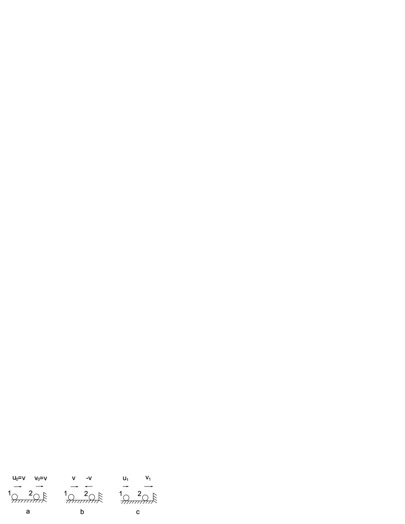
Figure 1: A scheme used to simulate the quantum search algorithm using classical collisions The two balls of masses $m_{1}$ and $m_{2}$ are moving with the same velocity along a horizontal and straight path without friction (Fig.1a). After ball 2 collides with the obstacle at the right end of the path, its velocity is inverted (Fig.1b). After the collision of the two balls, the velocities become $u_{1}$ and $v_{1}$ (Fig.1c).

In order to invert the velocity, we set an obstacle at the right end of the path. The velocity of ball 2 is inverted but its modulus remains unaltered after it collides with the obstacle. The velocities of the two balls after the collision are $v$ and $-v$ as shown in Fig.1b. This collision is analogous to the operation of $C$ used in the quantum searching algorithm. After ball 2 collides with the obstacle, it collides with ball 1. The second collision is analogous to operation by $D$. The velocities after this collision are $u_{1}$ and $v_{1}$ as shown in Fig.1c. The two collisions that are analogous to $C$ and $D$ constitute the complete iteration analogous to $U$ used in the quantum searching. There are 3 possible cases after the collision of the two balls: 1) The two balls both move rightwards, 2) ball 1 moves leftwards and ball 2 moves rightwards, and 3) the two balls both move leftwards. In some cases, the next collision of two balls cannot happen after the velocity of ball 2 is inverted again. Because we only are concerned with collisions and have no interest in the positions of the two balls, we can exchange the two balls’ positions or set an obstacle at the left end of the path in order to make the iteration continue. Assuming the two balls have velocities $u_{n}$ and $v_{n}$ after $n$ iterations, we obtain the recursion equations in matrix notation

$$\left(\begin{array}[]{cc}u_{n+1}\\ v_{n+1}\end{array}\right)=\left(\begin{array}[]{cc}{N_{1}-N_{2}}\over N_{1}+N_{2}&{-2N_{2}}\over N_{1}+N_{2}\\ {2N_{1}}\over N_{1}+N_{2}&{N_{1}-N_{2}}\over N_{1}+N_{2}\end{array}\right)\left(\begin{array}[]{c}u_{n}\\ v_{n}\end{array}\right),$$ (13)

by replacing the subscripts 1 and 0 in Eqs.(9) and (10) by $n+1$ and $n$, respectively, and by using the conditions that $m_{1}=N_{1}m_{0}$, and $m_{2}=N_{2}m_{0}$. For the quantum system, after $U$ is repeated $n$ times, the amplitudes in the collective state and marked state are transformed to $a_{n}$ and $b_{n}$. One can directly obtain the recursion equations

$$\left(\begin{array}[]{c}a_{n+1}\\ b_{n+1}\end{array}\right)=\left(\begin{array}[]{cc}{N_{1}-N_{2}}\over{N_{1}+N_{2}}&{-2N_{2}}\over{N_{1}+N_{2}}\\ {2N_{1}}\over{N_{1}+N_{2}}&{N_{1}-N_{2}}\over{N_{1}+N_{2}}\end{array}\right)\left(\begin{array}[]{c}a_{n}\\ b_{n}\end{array}\right)$$ (14)

from Eq.(13), based on the above-mentioned similarities. The initial conditions are $u_{0}=v_{0}=v$ for Eq.(13), and $a_{0}=b_{0}=1/\sqrt{N}$ for Eq.(14). The $2\times 2$ matrix in Eq.(14) is the product of Grover’s diffusion operator and suitable inversion operator, and is denoted by

$$T=\left(\begin{array}[]{cc}{N_{1}-N_{2}}\over{N_{1}+N_{2}}&{-2N_{2}}\over{N_{1}+N_{2}}\\ {2N_{1}}\over{N_{1}+N_{2}}&{N_{1}-N_{2}}\over{N_{1}+N_{2}}\end{array}\right).$$ (15)

We will proceed to solve Eqs.(13) and (14) using linear algebra [12]. One finds that

$$\left(\begin{array}[]{cc}u_{n}\\ v_{n}\end{array}\right)=T^{n}\left(\begin{array}[]{cc}u_{0}\\ v_{0}\end{array}\right),$$ (16)

$$\left(\begin{array}[]{c}a_{n}\\ b_{n}\end{array}\right)=T^{n}\left(\begin{array}[]{c}a_{0}\\ b_{0}\end{array}\right),$$ (17)

where $n=1,2,\cdots$. In order to obtain explicit expressions for $u_{n}$, $v_{n}$, $a_{n}$ and $b_{n}$, we transform $T$ to the diagonal matrix

$$T_{D}=S^{-1}TS\equiv\left(\begin{array}[]{cc}\lambda_{+}&0\\ 0&\lambda_{-}\end{array}\right).$$ (18)

The eigenvalues $\lambda_{\pm}$ of the matrix $T$ are the solutions of $\det(T-\lambda I)=0$. They can be expressed as

$$\lambda_{\pm}=\begin{array}[]{c}{N_{1}-N_{2}\pm 2i\sqrt{N_{1}N_{2}}}\over{N_{1}+N_{2}}\end{array}.$$ (19)

$S$ and $S^{-1}$ are expressed as

$$S=\left(\begin{array}[]{cc}1&1\\ -i\sqrt{{N_{1}}\over{N_{2}}}&i\sqrt{{N_{1}}\over{N_{2}}}\end{array}\right),$$ (20)

$$S^{-1}=\frac{1}{2}\left(\begin{array}[]{cc}1&i\sqrt{{N_{2}}\over{N_{1}}}\\ 1&-i\sqrt{{N_{2}}\over{N_{1}}}\end{array}\right).$$ (21)

One can easily find that

$$T^{n}=ST_{D}^{n}S^{-1}.$$ (22)

If $N_{2}=1$, and $N\gg 1$, $T_{D}$ can be expressed as

$$T_{D}=\left(\begin{array}[]{cc}e^{i2\theta}&0\\ 0&e^{-i2\theta}\end{array}\right),$$ (23)

using $\tan 2\theta\approx 2\theta$, where $\theta\equiv\frac{1}{\sqrt{N}}$. Using Eqs.(20)-(23), one can derive that

$$T^{n}=\left(\begin{array}[]{cc}\cos(2n\theta)&-\frac{1}{\sqrt{N-1}}\sin(2n\theta)\\ \sqrt{N-1}\sin(2n\theta)&\cos(2n\theta)\end{array}\right).$$ (24)

Using Eqs.(16), (17) and (24), we obtain the explicit expressions

$$\left(\begin{array}[]{cc}u_{n}\\ v_{n}\end{array}\right)=\left(\begin{array}[]{c}v\frac{\sqrt{N}}{\sqrt{N-1}}cos((2n+1)\theta)\\ v\sqrt{N}sin((2n+1)\theta)\end{array}\right),$$ (25)

$$\left(\begin{array}[]{cc}a_{n}\\ b_{n}\end{array}\right)=\left(\begin{array}[]{c}\frac{1}{\sqrt{N-1}}cos((2n+1)\theta)\\ sin((2n+1)\theta)\end{array}\right),$$ (26)

noting that $\sin\theta\approx\frac{1}{\sqrt{N}}$, and $\cos\theta\approx\sqrt{\frac{N-1}{N}}$. During the course of collisions, energy is transferred between the two balls through the change of their velocities. Let $n_{0}\approx(\pi\sqrt{N}/4-1/2)$ be the integer obtained by rounding $(\pi\sqrt{N}/4-1/2)$. When $n=n_{0}$, ball 2 can acquire almost all the mechanical energy of the system. Correspondingly, for the quantum searching algorithm, the amplitude in the marked state can approach 1 if the number of repetitions of $U$ is $n_{0}$. The quantum system lies in the marked state if a measurement is made. Our results show agreements with Refs.[4][13][14]. We now discuss some related problems based on these discussed similarities.

1.Simulating Grover quantum searching algorithm on a classical system Because $p_{i}$ is analogous to $|i>$, a system consisting of $2^{n}$ particles $p_{i}(i=0,1,2,...,2^{n}-1)$ can be used to simulate a quantum system that stores $n$ qubits of information. For example, if $m_{1}=3m_{0}$ and $m_{2}=m_{0}$, the classical system can simulate a two qubit system with $N_{1}=3$, $N_{2}=1$, and $N=4$. After exactly one iteration, we find that $u_{1}=0$, $v_{1}=2v$. This result means that ball 2 obtains all the energy of the system, which is analogous to the probability equal to 1 of getting the marked state. Our result is in agreement with the result demonstrated on an NMR quantum computer [5]. If $m_{1}=7m_{0}$, and $m_{2}=m_{0}$, the following results are obtained:

$$\left(\begin{array}[]{c}u_{1}\\ v_{1}\end{array}\right)=\left(\begin{array}[]{c}1/2\\ 5/2\end{array}\right)v,$$ (27)

$$\left(\begin{array}[]{c}u_{2}\\ v_{2}\end{array}\right)=\left(\begin{array}[]{c}-1/4\\ 11/4\end{array}\right)v.$$ (28)

Ball 2 nearly gets the entire energy of the system after 2 iterations. Because mass is continuous, the case where $m_{2}=m_{0}$, and $m_{1}=N_{1}m_{0}$ is equivalent to the case where $m_{2}=km_{0}$, and $m_{1}=kN_{1}m_{0}$ ($k$ is a positive integer). The case where $m_{1}=3m_{0}$, and $m_{2}=m_{0}$ is analogous to the case where $N_{2}=N/4$ as discussed in Ref. [4], in which after one iteration, the probability of getting the marked state is 1. If we choose the condition that $m_{1}/m_{2}=p/q$, where $q\neq 1$, and $p$ and $q$ are positive integers with no common factor, we can simulate the quantum search algorithm in the case where the marked state contains multiple basis states, which cannot be realized by NMR [15].

2. Limits on quantum searching Because the two balls exchange their energy after they collide with each other, neither of them can get all the energy of the system if $m_{1}=m_{2}$. This case is analogous to the case where the search algorithm is invalid, more specifically, where $N_{1}=N_{2}$ [16]. We also find that

$$\left(\begin{array}[]{c}u_{1}\\ v_{1}\end{array}\right)=\left(\begin{array}[]{c}1-4N_{2}/N\\ 3-4N_{2}/N\end{array}\right)v,$$ (29)

using the initial condition $u_{0}=v_{0}=v$. Eq.(29) means that if $N_{2}>N/4$, the velocity of ball 1 is inverted after the first iteration. It is possible that the two balls move in the same direction after the velocity of ball 2 is inverted in the second iteration. The energy of ball 2 is reduced after it catches up with ball 1 and collides with it. In this case, the searching algorithm is not efficient [16].

3.Qualitative discussion of the needed number of iterations Considering the case where $m_{2}=m_{0}$, $m_{1}=(N-1)m_{0}$. The initial condition is $u_{0}=v_{0}=v$, and $N\gg 1$. We obtain $u_{1}\approx v$, and $v_{1}=3v$ after the first iteration. This means that the velocity of ball 2 increases by $2v$ and the velocity of ball 1 hardly change in any iteration. The velocity of ball 2 increases by $2nv$ after $n$ iterations. When $n\approx\sqrt{N}/2$, ball 2 gets almost all energy of the system.

Acknowledgement This work is supported by the National Nature Science Foundation of China. We are also grateful to Professor Shouyong Pei of Beijing Normal University for his helpful discussions on the principle of quantum algorithm.

References

- [1] D. Deutsch, and A. Ekert, Introduction to quantum computation, in The Physics of quantum Information,edited by D. Bouwmeester, A.Ekert, and A. Zeilinger. (Springer,Berlin Heidelberg,2000)pp.93-132.
- [2] L.K. Grover,Quantum mechanics helps in searching for a needle in a haystack, Phys.Rev.Lett.79,325 (1997)
- [3] S. Yu, and C.Sun, Quantum searching’s underlying SU(2) structure and its quantum decoherence effect, quant-ph/9903075;C. Sun, X. Yi, D. Zhou, and S. Yu.Problems on quantum decoherence,in The new progress of quantum mechanics (in Chinese)(Peking University publishing house,Beijing,2000).
- [4] M. Boyer,G. Brassard,P Hyer,and A.Tapp, Tight bounds on quantum searching, e-print quant-ph/9605034;Fortsch.phys.46,493(1998)
- [5] I. L. Chuang,N. Gershenfeld,and M. Kubinec, Experimental implementation of fast quantum searching. Phys.Rev.Lett. 80,3408 (1998)
- [6] L.K. Grover,Quantum computers can search rapidly by almost any transformation, Phys.Rev.Lett.80,4329(1998)
- [7] J.Zhang,Z.Lu,L.Shan,and Z.Deng,Realization of generalized quantum searching using nuclear magnetic resonance, Phys.Rev.A. 034301 (2002)
- [8] L.K. Grover, From schrodinger’s equation to the quantum search algorithm, Am. J.Phys. 69(7),769(2001)
- [9] L. K. Grover,and A.M.sengupta, A classical analog of quantum search, e-print quant-ph/0109123.
- [10] R. Jozsa,Searching in Grover’s algorithm, quant-ph/9901021
- [11] H. D. Young, Fundamentals of Mechanics and heat(Mcgraw-hill BOOK company, New York,1974)
- [12] E.Biham,O.Biham,D.Biron,M.Grassl,D.A.Lidar,and D.Shapira, Analysis of generalized Grover quantum search algorithms using recursion equations, Phys.Rev. A,63,012310(2000)
- [13] E.Farhi,and S.Gutmann,Analog analogue of a digital quantum computation, Phys.Rev. A,57,2403(1998)
- [14] G. Chen, S.A.Fulling, and M.O.Scully, Grover’s algorithm for multiobject search in quantum computing, quant-ph/9909040
- [15] J. A. Jones, and M. Mosca,Approximate quantum counting on an NNR ensemble quantum computer, Phys.Rev.Lett.83,1050(1999)
- [16] L. K. Grover,Quantum computers can search arbitrarily large databases by a single query, Phys.Rev.Lett.79,4709(1997)