Realization of generalized quantum searching using nuclear magnetic resonance

The quantum searching algorithm was first proposed by Grover [1]. It can speed up some search applications over unsorted data and has been become a hot topic in quantum information [2$\sim$5]. The surprising result of the algorithm is that searching a particular item in unsorted list of N elements only requires $O(\sqrt{N})$ attempts [2]. The algorithm needs the properties of Walsh-Hadamard(W-H) transform and has been implemented using NMR techniques [6]. Grover generalized the algorithm in theory, in which the Walsh-Hadmamard transform can be replaced by almost any quantum operation [7].

The generalized algorithm can be posed as follows. If a unitary operator U is applied to a quantum system in an initial basis state $|\gamma>$, the system lies in a superposition $\sum_{i}a_{i}|i>$, where $a_{i}=<i|U|\gamma>=U_{i\gamma}$. The amplitude of reaching the target state $|\tau>$ is $U_{\tau\gamma}$, and the probability of getting the system in state $|\tau>$ is $|U_{\tau\gamma}|^{2}$ if a measurement is made. Therefore, it will take at least $O(1/|U_{\tau\gamma}|^{2})$ repetitions of U and the measurement to get state $|\tau>$ for one time. In contrary, according to the generalized searching algorithm, in $O(1/|U_{\tau\gamma}|)$ applications, operator Q transforms $|\gamma>$ into $U^{-1}|\tau>$. After U is applied, the system lies in state $|\tau>$. Q is defined as $Q\equiv-I_{\gamma}U^{-1}I_{\tau}U$, where $I_{i}\equiv I-2|i><i|$, and I denotes unit matrix. If $I_{i}$ is applied to a superposition of states, it only inverts the amplitude in state $|i>$, and leaves the other states unaltered. It has been showed in theory that the number of repetitions of Q required to transform $|\gamma>$ into $|\tau>$ is $\pi/4|U_{\tau\gamma}|$ if $|U_{\tau\gamma}|\ll 1$.

It can be proved that for a two qubit system, the number of repetitions of Q is also $O(1/|U_{\tau\gamma}|)$ without the condition that $|U_{\tau\gamma}|\ll 1$. Particularly, if $|U_{\tau\gamma}|=1/2$, the number of repetitions is 1, and the probability of getting the target state is 1. In this paper, we will implement the generalized quantum algorithm in this case on a two qubit NMR quantum computer [8].

Our experiments use a sample of Carbon-13 labelled chloroform (Cambridge Isotopes) dissolved in d6-acetone. Data are taken at controlled temperature (22${}^{0}C$) with a Bruker DRX 500 MHz spectrometer (Beijing Normal University). The resonance frequencies $\nu_{1}=125.76$ MHz for ${}^{13}C$, and $\nu_{2}=500.13$ MHz for ${}^{1}H$. The coupling constant $J$ is measured to be 215 Hz. If the magnetic field is along $\hat{z}$-axis, and let $\hbar=1$, the Hamitonian of this system is

$$H=-2\pi\nu_{1}I_{z}^{1}-2\pi\nu_{2}I_{z}^{2}+2\pi JI_{z}^{1}I_{z}^{2},$$ (1)

where $I_{z}^{k}(k=1,2)$ are the matrices for $\hat{z}$-component of the angular momentum of the spins [9]. In the rotating frame of spin k, the evolution caused by a radio-frequency(rf) pulse along $\hat{x}$ or $\hat{y}$-axis is denoted as $X_{k}(\varphi_{k})=e^{i\varphi_{k}I_{x}^{k}}$ or $Y_{k}(-\varphi_{k})=e^{-i\varphi_{k}I_{y}^{k}}$, where $\varphi_{k}=B_{1}\gamma_{k}t_{p}$. $B_{1}$, $\gamma_{k}$ and $t_{p}$ represent the strength of magnetic field, gyromagnetic ratio of spin k and the width of the rf pulse, respectively. The pulse used above is denoted as $[\varphi]_{x}^{k}$ or $[-\varphi]_{y}^{k}$. The coupled-spin evolution is denoted as

$$[t]=e^{-i2\pi JI_{z}^{1}I_{z}^{2}},$$ (2)

where t is evolution time. The pseudo-pure initial state

$$|\gamma>=|\uparrow>_{1}|\uparrow>_{2}=\left(\begin{array}[]{c}1\\ 0\\ 0\\ 0\end{array}\right)$$ (3)

is prepared by using spatial averaging [10], where $|\uparrow>_{k}$ denotes the state of spin k. For convenience, the notion $|\uparrow>_{1}|\uparrow>_{2}$ is merged into $|\uparrow\uparrow>$ and the subscripts 1 and 2 are omitted. The basis states are arrayed as $|\uparrow\uparrow>,|\uparrow\downarrow>,|\downarrow\uparrow>$, $|\downarrow\downarrow>$. In matrix notion, $I_{i}$ is a diagonal matrix with all diagonal terms equal to 1 except the $ii$ term which is -1. For example, if $|i>=|\downarrow\downarrow>$, $I_{i}$ is expressed as

$$I_{3}=\left(\begin{array}[]{cccc}1&0&0&0\\ 0&1&0&0\\ 0&0&1&0\\ 0&0&0&-1\end{array}\right).$$ (4)

U is chosen as three forms

$$U_{1}=1/2\left(\begin{array}[]{cccc}-1&-1&-1&-1\\ -1&1&-1&1\\ -1&-1&1&1\\ -1&1&1&-1\end{array}\right),$$ (5)

$$U_{2}=1/2\left(\begin{array}[]{cccc}1&1&1&1\\ -1&1&-1&1\\ -1&-1&1&1\\ 1&-1&-1&1\end{array}\right)$$ (6)

and

$$U_{3}=1/2\left(\begin{array}[]{cccc}1&i&i&-1\\ i&1&-1&i\\ i&-1&1&i\\ -1&i&i&1\end{array}\right),$$ (7)

where $U_{1}$ is the W-H transform used in reference [6] (up to an phase factor). It is easily proved that $UQ$ can transform state $|\gamma>$ into state $|\tau>$. The irrelevant overall phase factors are ignored.

The evolution of the system can be represented by its deviation density matrix $\rho_{\Delta}$[11]. For the heteronuclear system, the following rf and gradient pulse sequence $[\alpha]_{x}^{2}-[grad]_{z}-[\pi/4]_{x}^{1}-1/4J-[\pi]_{x}^{1}-[\pi]_{x}^{2}-1/4J-[-\pi/4]_{y}^{1}-[grad]_{z}$ transforms the system from the equilibrium state

$$\rho_{\Delta eq}=\gamma_{1}I_{z}^{1}+\gamma_{2}I_{z}^{2}$$ (8)

to the initial state required in experiments

$$\rho_{\Delta 0}=-(I_{z}^{1}/2+I_{z}^{2}/2+I_{z}^{1}I_{z}^{2})=-1/4\left(\begin{array}[]{cccc}3&0&0&0\\ 0&-1&0&0\\ 0&0&-1&0\\ 0&0&0&-1\end{array}\right),$$ (9)

where $\alpha=\arccos(\gamma_{1}/2\gamma_{2})$, and $[grad]_{z}$ denotes gradient pulse along $\hat{z}$-axis. The pulses are applied from left to right. The symbol 1/4J denotes the evolution caused by the Hamitonian H for 1/4J without pulses. The initial state can be used as the pseudo-pure state $|\uparrow\uparrow>$ in NMR quantum computation [12]. By applying pulse $[\pi]_{x}^{2}$, $[\pi]_{x}^{1}$ or $[\pi]_{x}^{1}[\pi]_{x}^{2}$, the pseudo- pure states corresponding to states $|\uparrow\downarrow>$, $|\downarrow\uparrow>$ or $|\downarrow\downarrow>$ can be gotten. They are written as

$$\rho_{\Delta 1}=-(I_{z}^{1}/2-I_{z}^{2}/2-I_{z}^{1}I_{z}^{2})$$ (10)

$$\rho_{\Delta 2}=-(-I_{z}^{1}/2+I_{z}^{2}/2-I_{z}^{1}I_{z}^{2})$$ (11)

$$\rho_{\Delta 3}=-(-I_{z}^{1}/2-I_{z}^{2}/2+I_{z}^{1}I_{z}^{2})$$ (12)

We also represent the four pseudo- pure states above as $|\uparrow\uparrow>,|\uparrow\downarrow>,|\downarrow\uparrow>,$ and $|\downarrow\downarrow>$, respectively. According to reference[6], we find that

$I_{0}=Y_{1}(\pi/2)Y_{2}(\pi/2)X_{1}(-\pi/2)X_{2}(-\pi/2)Y_{1}(-\pi/2)Y_{2}(-\pi/2)[1/2J]$,

$I_{1}=Y_{1}(\pi/2)Y_{2}(\pi/2)X_{1}(\pi/2)X_{2}(-\pi/2)Y_{1}(-\pi/2)Y_{2}(-\pi/2)[1/2J]$,

$I_{2}=Y_{1}(\pi/2)Y_{2}(\pi/2)X_{1}(-\pi/2)X_{2}(\pi/2)Y_{1}(-\pi/2)Y_{2}(-\pi/2)[1/2J]$ and

$I_{3}=Y_{1}(\pi/2)Y_{2}(\pi/2)X_{1}(\pi/2)X_{2}(\pi/2)Y_{1}(-\pi/2)Y_{2}(-\pi/2)[1/2J]$. The time order is from right to left. It is easy to prove that

$U_{1}=X_{1}(\pi)X_{2}(\pi)Y_{1}(-\pi/2)Y_{2}(-\pi/2)$,

$U_{2}=Y_{1}(\pi/2)Y_{2}(\pi/2)$, and

$U_{3}=X_{1}(\pi/2)X_{2}(\pi/2)$.

In our experiments, each NMR spectrum of spin k is obtained by a spin-selective readout pulse $[-\pi/2]_{y}^{k}$. The relative phases of signals are meaningful because all experiments are acquired in an identical fashion [13]. At first, we prepare the four pseudo- pure states described in equations(9)-(12). For the system in a pseudo- pure state, only one NMR peak appears in a spectrum if a selective readout pulse is applied. Fig.1 shows the experimental MNR spectra when the system lies in various pseudo- pure states. Figs.1a, b, c and d are spectra when the system lies in pseudo- pure states $|\uparrow\uparrow>,|\uparrow\downarrow>,|\downarrow\uparrow>$ and $|\downarrow\downarrow>$, respectively. In each figure, the main spectrum represents the spectrum of ${}^{13}C$ and the ${}^{1}H$ spectrum is a smaller inset. For each experiment, the initial state $|\gamma>$ is pseudo- pure state $|\uparrow\uparrow>$. U is selected as $U_{1},U_{2}$ or $U_{3}$. The searching state $|\tau>$ can be any pseudo- pure state. $UQ$ transforms state $|\gamma>$ into state $|\tau>$. Therefore, the number of application of Q is 1. The searching results on condition that $U=U_{3}$ and $|\tau>=|\uparrow\uparrow>$, $|\uparrow\downarrow>$, $|\downarrow\uparrow>$, or $|\downarrow\downarrow>$ are shown in Fig.2. Comparing Figs.2a, b, c and d with Figs.1a, b, c and d respectively, we confirm that the system truly lies in the target state. In order to illustrate that the searching results for $U_{3}$ are the same as $U_{1}$ or $U_{2}$, Fig.3 shows the searching results on condition that $|\tau>=|\uparrow\downarrow>$, and $U=U_{1}$ (shown by Fig.3a) or $U_{2}$ (shown by Fig.3b). It can be found from various spectra that the experimental errors are not lager than 5 percent expect only two ${}^{1}H$ spectra. The errors mainly result from the imperfection of pulses, inhomogeneity of magnetic field and effect of decoherence. We find that if each $[\pi/2]_{\phi}^{k}$ ($\phi$=x or y) in $I_{i}$ is replaced by $[-\pi/2]_{\phi}^{k}$, and each $[-\pi/2]_{\phi}^{k}$ is replaced by $[\pi/2]_{\phi}^{k}$, the results remain the same. This fact can be used to simplify pulse sequences and reduce experimental errors.

In conclusion, we demonstrate the generalized quantum searching algorithm by replacing W-H transform by different transformations. Because the number of repetition of operator Q is determined by the element $|U_{\tau\gamma}|$ and these three U transformations have the same $|U_{\tau\gamma}|$, it is not surprised that the numbers of repetitions of Q are all 1. Compared with temporal labelling, the spatial averaging used to prepare initial state shortens experiment time. It only takes about 2 minutes to finish one experiment. The searching results can be directly read out from spectra, so that the steps of recording areas of peaks are avoided. These facts simplify the process of experiments and make the searching results easy to observe.

This work was partly supported by the National Nature Science Foundation of China. We are also grateful to Professor Shouyong Pei of Beijing Normal University for his helpful discussions on the principle of quantum algorithm and also to Dr. Jiangfeng Du of University of Science and Technology of China for his helpful discussions on experiment.

Figure Captions

1. The NMR spectra of ${}^{13}C$(main figures) and ${}^{1}H$ (smaller insets), when the two-spin system lies in various pseudo- pure states via readout pulses selective for ${}^{13}C$ (main figures) and ${}^{1}H$(smaller insets). The amplitude has arbitrary units. When the system lies in a pseudo-pure state, only one NMR peak appears in the spectrum of spin k if a readout pulse $[-\pi/2]_{y}^{k}$ is applied. Figs.1a, b, c and d are spectra corresponding to pseudo- pure states $|\uparrow\uparrow>,|\uparrow\downarrow>,|\downarrow\uparrow>$and $|\downarrow\downarrow>$, respectively.

2. Spectra of ${}^{13}C$ (main figures) and ${}^{1}H$ (smaller insets) after completion of the generalized searching algorithm and readout pulses selective for ${}^{13}C$ (main figures) and ${}^{1}H$ (smaller insets). U is chosen as $U_{3}$, and the target state $|\tau>$ is $|\uparrow\uparrow>,|\uparrow\downarrow>,|\downarrow\uparrow>$ or $|\downarrow\downarrow>$. The corresponding searching results are shown by Figs.2a, b, c or d. By comparing Figs.2a, b, c and d with Figs.1a, b, c and d respectively, we confirm that the system is truly in the target state.

3. Spectra of ${}^{13}C$ (main figures) and ${}^{1}H$ (smaller insets) after completion of the generalized searching algorithm and readout pulses selective for ${}^{13}C$ (main figures) and ${}^{1}H$ (smaller insets) on condition that $|\tau>=|\uparrow\downarrow>$, and $U=U_{1}$ shown by Fig.3a or $U=U_{2}$ shown by Fig.3b.

1

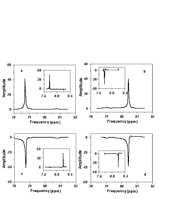
Figure 1:

2

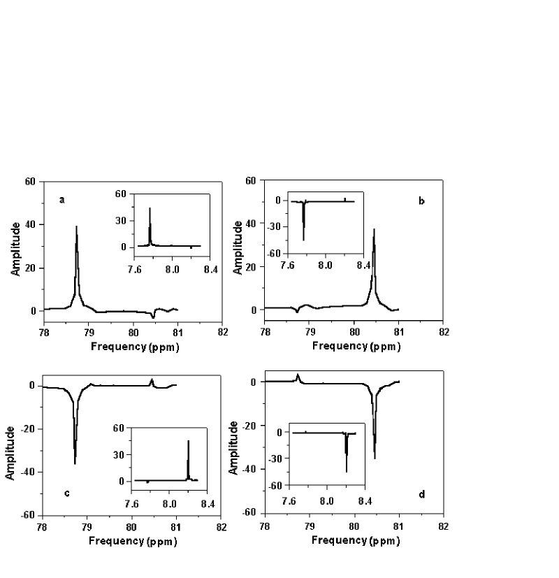
Figure 2:

3

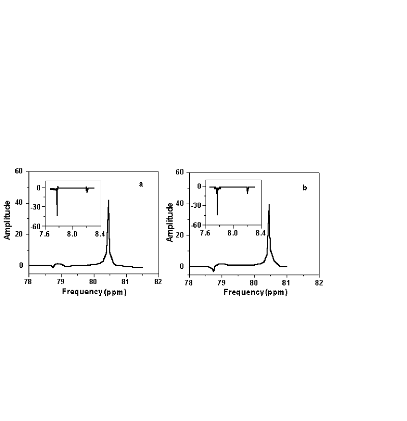
Figure 3:

References

• [1] L.K.Grover,Phys.Rev.Lett.79,325 (1997)
• [2] M. Boyer,G. Brassard,FRSC, P H$\phi$yer,and A.Tapp, LANL e-print quant-ph/9605034; Fortsch. phys. 46,493(1998))
• [3] C.Zalka, LANL e-print quant-ph/9711070; Phys. Rev. A,60,2746(1999)
• [4] L.K.Grover,Phys.Rev.Lett.79,4709(1997)
• [5] L.K.Grover,Phys.Rev.Lett.85,1334(2000)
• [6] I. L.Chuang,N. Gershenfeld,and M. Kubinec. Phys.Rev.Lett. 80,3408 (1998)
• [7] L.K.Grover,Phys.Rev.Lett PRL,80,4329(1998)
• [8] L. M.K. Vandersypen,C.S.Yannnoni,and I.L.Chuang,quant-ph/0012108
• [9] R.R.Ernst,G.bodenhausen and A.Wokaum,Principles of nuclear magnegtic resonance in one and two dimensions, Oxford University Press(1987)
• [10] D.G.Cory,M.D.Price,and T.F.Havel,Physica D.120,82 (1998)
• [11] I. L.Chuang, N.Gershenfeld,M.G.Kubinec and D.W.Leung, Proc.R.Soc.Lond.A 454,447 (1998)
• [12] E.Knill,I.Chuang, and R.Laflamme,Phys.Rev.A 57,3348 (1998)
• [13] J. A. Jones,in The Physics of quantum Information,edited by D. Bouwmeester, A.Ekert, and A. Zeilinger. (Springer,Berlin Heidelberg,2000)pp.177-189.