Abstract:This paper presents some results on some aspects of the two-level atom interacting with a single-mode with the privileged field mode being in the squeezed displaced Fock state (SDFS). The exact results are employed to perform a careful investigation of the temporal evolution of the atomic inversion, entropy and phase distribution. It is shown that the interference between component states leads to non-classical oscillations in the photon number distribution. At mid revival time the field is almost in the pure state. We have briefly discussed the evolution of the Q function of the cavity field. The connection between the field entropy and the collapses and revivals of the atomic inversion has been established. We find that the phase probability distribution of the field reflect the collapses and revivals of the level occupation probabilities in most situations. The interaction brings about the symmetrical splitting of the phase probability distribution. The general conclusions reached are illustrated by numerical results.

PACS: 39.20.+q, 42.50.Vk, 32.80.-t, 03.65.Ge

To be published in Physics Scripta

1 Introduction

The entropy of a radiation field is one of the canonical problems of statistical physics and has attracted much attention in the past. In recent years much attention has been focused on the properties of the entanglement between the field and the atom and in particular the entropy of the system [1-11]. The authors in [2-4] have shown that entropy is a very useful operational measure of the purity of the quantum state, which automatically includes all moments of the density operator. The time evolution of the field (atomic) entropy reflects the time evolution of the degree of entanglement between the atom and the field. The higher the entropy, the greater the entanglement.

The concept of the photon in the quantum theory of a radiation field has been built on the number (Fock) state $|n\rangle$. However, another important state is the coherent state which is a linear superposition of all $|n\rangle$ states with coefficients chosen such that the photon number distribution is Poissonian. It may be defined by the action of a displacement operator $D(\alpha)$ on the vacuum state. This state has been extensitevly studied [12-14]. On the other hand the squeezed state is one of the non-classical states of the electromagnetic field in which certain observables exhibit fluctuations less than in the vacuum state [15-17]. It is defined by the action of the squeeze operator $S(z)$ on the coherent state [15-17]. Squeezed displaced Fock states (SDFS) have been introduced and different aspects of these states such as squeezing and photon statistics have been investigated [18-25]. These states generalize two-photon coherent states [17] (squeezed coherent states), squeezed number states [18], and displaced Fock states [26-28]. They exhibit both number and quadrature squeezing. Recently the creation of nonclassical states of motion of a trapped ion such as Fock states, coherent states, squeezed states and Schrödinger-cat states have been reported [29-31]. In these experiments an ion is laser-cooled in a Paul trap to the ground harmonic state. Then the atom is put into various quantum states of motion by applications of optical and electric fields. That moved the study of these states from the academic realm to the world of experimentation. This motivated us to study the interaction of these states with a two-level atom.

A stochastic formulation of quantum mechanics involves, basically, two interrelated problems. These are the determination of the probability functions of the density operator, ${\rho}$, and the establishment of the proper correspondence between quantum-mechanical observable, and ordinary functions in phase-space. Attempts in this direction ran into the difficulty of dealing with quasidistributions,[32-33]. The three types of quasiprobability distribution functions P, Q and W (for normal, antinormal and symmetric ordering respectively) are very important in quantum optics [32-33].

Recently Pegg and Barnett [34, 35] have introduced a new hermitian phase formalism which successfully overcomes the troubles inherent in the Susskind-Glogower phase formalism and enables one to study finer detials of the phase properties of quantum fields. Such quantities as expectation values and variances of the hermitian phase operators or phase distribution functions are now available for investigation [36, 37]. One of our interests is to investigate the phase properties here.

The material of this paper is arranged as follows: In section 2, we review a few concepts of squeezed displaced Fock states (SDFS’s). In section 3 we introduce the model and write the expressions for the final state vector at any time $t>0$. We discuss the field entropy in section 3.1. By numerical computations, we examine the influence of the SDFS’s on the field entropy evolution and entanglement of the atom and the field. We analyse oscillations in the photon number distribution of the cavity field in section 3.2. Section 3.3 discuss the phase probability distribution through the framework of Pegg-Barnett’s definition of the Hermitian phase operator. We present the evolution of the Q function for the SDFS’s in section 3.4. Finally, summary and remarks are presented.

2 Squeezed displaced Fock states (SDFS’s)

The SDFS’s are generated from the number state $|m\rangle$ as shown below. These states have been studied extensively in literature, because of their interesting nonclassical properties and expected prospective applications in optical communication and interferometery [14]. The SDFS is defined by [18-25]

$${|}{\alpha_{0}},z,m{\rangle}=D({\alpha_{0}})S(z){|}m{\rangle}$$ (1)

where the displacement operator $D({\alpha_{0}})$ ,( with $\alpha_{0}$ a complex parameter that represents the magnitude and angle of the displacement) [12-13], and the squeeze operator $S(z)$ are given by [14-17]

$$D({\alpha_{0}}) = \exp({\alpha_{0}}{a^{+}}-{{\alpha_{0}}^{*}}a),$$

$$S(z) = \exp[{\frac{z^{*}}{2}a^{2}}-{\frac{z}{2}{{a^{+}}^{2}}}],$$ (2)

where $z=re^{i\phi}$ and $r$ is known as the squeeze parameter and $\phi$ indecates the direction of the squeezeing, with $a$ $(a^{+})$ are the annihilation (creation) operators of the field.

It is easy to calculate the average value of the number operator, ${a^{+}}a$, in the state ${|}{\alpha_{0}},z,m{\rangle}$, by using the above relations, thus

$${\langle}{a^{+}}a{\rangle}=({|}{\mu}{|}^{2}+{|}{\nu}{|}^{2})m+{|}{\nu}{|}^{2}+{|}{{\alpha_{0}}}{|}^{2},$$ (3)

where $\mu=\cosh{r}$, and $\nu=\exp(i\phi)\sinh{r}$.

The photon number distributions $P_{n}$ for ${|}{\alpha_{0}},z,m{\rangle}$ is equal to the square of the absolute value of the matrix elements ${\langle}n{|}{\alpha},z,m{\rangle}$. The analytical expression for ${\langle}n{|}{\alpha},z,m{\rangle}$ is given by [19],

$${\langle}n{\mid} {\alpha_{0}},z,m{\rangle}=({\frac{n!}{{\mu}m!}})^{1/2}({\frac{\nu}{2\mu}})^{n/2}\exp(-\frac{{\mid}{\bar{\alpha}_{0}}{\mid}^{2}}{2}+\frac{{\nu}^{*}}{2{\mu}}{\bar{\alpha}_{0}}^{2})$$ (4)

$$\times{\sum_{i=0}^{min(n,m)}}{(^{m}_{i})}\frac{({\frac{2}{\mu\nu})}^{i/2}}{(n-i)!}[(\frac{-{\nu}^{*}}{2\mu})^{\frac{m-i}{2}}$$

$$\times]{H_{n-i}[{\frac{\bar{\alpha}_{0}}{(2{\nu}{\mu})^{1/2}}]}{H_{m-i}[{\frac{-{\alpha_{0}}^{*}}{(-2{\nu^{*}}{\mu})^{1/2}}]}}},$$

where $\bar{\alpha}_{0}=\mu\alpha_{0}+\nu{\alpha_{0}}^{*}$, and $H_{n}(x)$ stands for the Hermite function of order $n$ [38]. Therefore, the photon number distribution ${P_{n}}$ is given by

$$P_{n}={{|}{\langle}{n}{|}{\alpha_{0}},z,m{\rangle}{|}}^{2},$$ (5)

The scalar product of two different SDFS states $\langle\alpha_{1},z_{1},m_{1}|\alpha_{2},z_{2},m_{2}\rangle$ is very useful in the representation with SDFS basis. We can obtain it with the help of the completeness of coherent states as

$$\langle\alpha_{1},z_{1},m_{1}|\alpha_{2},z_{2},m_{2}\rangle=\frac{1}{\pi}\int\langle\alpha_{1},z_{1},m_{1}|\beta\rangle\langle\beta|\alpha_{2},z_{2},m_{2}\rangle\thinspace d^{2}\beta$$

By using equation (4),

$$\langle \alpha_{1},z_{1},m_{1}|\alpha_{2},z_{2},m_{2}\rangle=\frac{1}{\sqrt{m_{1}!m_{2}!\mu_{1}\mu_{2}K}}(-\frac{\nu_{2}^{*}}{2\mu_{2}})^{m_{2}/2}$$

$$\times(-\frac{\nu_{1}}{2\mu_{1}})^{m_{1}/2}\exp\biggl{[}-\frac{|\alpha_{2}|^{2}}{2}-\frac{|\alpha_{1}|^{2}}{2}\biggr{]}$$

$$\times\exp\biggl{[}\frac{1}{\mu_{2}\mu_{1}-\nu_{2}\nu_{1}^{*}}\alpha_{1}^{*}\alpha_{2}-\frac{\nu_{2}\mu_{1}-\mu_{2}\nu_{1}}{2(\mu_{2}\mu_{1}-\nu_{2}\nu_{1}^{*})}{\alpha_{1}^{*}}^{2}$$

$$+\frac{(\nu_{2}\mu_{1}-\mu_{2}\nu_{1})^{*}}{2(\mu_{2}\mu_{1}-\nu_{2}\nu_{1}^{*})}{\alpha_{2}}^{2}\biggr{]}\sum_{s=0}^{[m_{2}/2]}\sum_{\acute{s}=0}^{[m_{1}/2]}\sum_{r=0}^{min(m_{2}-2s,m_{1}-2\acute{s})}$$

$$\times\frac{m_{1}!m_{2}!(-1)^{s+\acute{s}}}{s!\acute{s}!r!}\biggl{[}\frac{2}{(-2\mu_{2}\nu_{2}^{*})^{1/2}}\biggr{]}^{m_{2}-2s}$$

$$\times\biggl{[}\frac{2}{(-2\mu_{1}\nu_{1})^{1/2}}\biggr{]}^{m_{1}-2\acute{s}}\frac{(1/K)^{r}}{(m_{2}-2s-r)!(m_{1}-2\acute{s}-r)!}$$

$$\biggl{(}\sqrt{\frac{\nu_{2}}{2K\mu_{2}}}\biggr{)}^{m_{1}-2\acute{s}-r}H_{m_{1}-2\acute{s}-r}$$

$$\times\biggl{[}\frac{(\alpha_{02}-\alpha_{01})-\frac{\nu_{2}}{\mu_{2}}(\alpha_{01}^{*}-\alpha_{02}^{*})}{2\sqrt{\frac{K\nu_{2}}{2\mu_{2}}}}\biggr{]}\biggl{(}\sqrt{\frac{\nu_{1}^{*}}{2K\mu_{1}}}\biggr{)}^{m_{2}-2s-r}$$

$$\times H_{m_{2}-2s-r}\biggl{[}\frac{(\alpha_{01}^{*}-\alpha_{02}^{*})-\frac{\nu_{1}^{*}}{\mu_{1}}(\alpha_{02}-\alpha_{01})}{2\sqrt{\frac{K\nu_{1}^{*}}{2\mu_{1}}}}\biggr{]}$$

where $K={\mu_{2}\mu_{1}-\nu_{2}\nu_{1}^{*}}/{\mu_{2}\mu_{1}}$ and $\alpha_{01}={\mu_{1}}\alpha_{1}-\nu_{1}\alpha_{1}^{*},$ $\alpha_{02}={\mu_{2}}\alpha_{2}-\nu_{2}\alpha_{2}^{*}$. An equivalent result (however not having the Hermite polynomials in the summand) has been given recently [24]. When $m_{1}=m_{2}=0$ the above equation gives the result in [16], for the squeezed state. But when $\nu_{1}=\nu_{2}=0$ and $\mu_{1}=\mu_{2}=1$ then this equation becomes

$$\langle\alpha_{1},m_{1}|\alpha_{2},m_{2}\rangle=\frac{\langle\alpha_{1}|\alpha_{2}\rangle}{\sqrt{m_{1}m_{2}}}\sum_{r=0}^{min(m_{1},m_{2})}$$

$$\times\frac{m_{2}!m_{1}!}{r!(m_{2}-r)!(m_{1}-r)!}(\alpha_{1}^{*}-\alpha_{2}^{*})^{m_{2}-r}(\alpha_{2}-\alpha_{1})^{m_{1}-r}$$

which is the result of, [28,18], for the displaced Fock state. Other special cases follow in a straightforward way.

3 The quantum dynamics

We consider the Hamiltonian for the one-photon Jaynes-Cummings model. It describes the interaction of a single-mode quantized field with a two-level atom via a one-photon process. The Hamiltonian of the system in the rotating-wave approximation is written as

$${\hat{H}}=\frac{1}{2}\omega_{\circ}\sigma_{z}+\omega{\hat{a}}^{\dagger}{\hat{a}}+\lambda({\hat{a}}\sigma_{+}+{\hat{a}}^{\dagger}\sigma_{-}),$$ (6)

where ${\hat{a}}^{\dagger}$ $({\hat{a}})$ is the creation (annihilation) operators for the photon of frequency $\omega,$ and $\lambda$  describes the coupling to the atomic system. The two level atom with transition frequency $\omega_{\circ}$ is described by the Pauli raising and ( lowering ) operators $\sigma_{+},(\sigma_{-})$ and the inversion operator $\sigma_{z}$. with the detuning parameter $\Delta=\omega-\omega_{\circ}$.

The initial state of the total atom-field system can be written as

$$\mid\psi(0)>=\psi(0)>_{f}\otimes\mid\psi(0)>_{a}=\sum_{n=0}q_{n}\mid n,e>,$$ (7)

means that the atom starts in its excited state, the field is assumed to be initially in the squeezed displaced Fock states(SDFS) $q_{n}=<n\mid\alpha_{0},z,m>$ given by Eq. (4). The solution of the Schrödinger equation in the interaction picture i.e the wave function of the system at any time $t>0$ is given by

$$\mid\psi(t)>=\sum_{n=0}^{\infty}\biggl{(}A_{n}(t)\mid n,e>+B_{n}(t)\mid n+1,g>\biggr{)},$$ (8)

where the coefficients $A_{n}$ and $B_{n}$ are given by the formulae

$$A_{n}(t)=q_{n}\biggl{(}\cos\lambda t\nu_{n}-\frac{i\Delta}{2\lambda}\frac{\sin\lambda t\nu_{n}}{\nu_{n}}\biggr{)},$$ (9)

$$B_{n}(t)=-iq_{n}\sqrt{n+1}\frac{\sin\lambda t\nu_{n}}{\nu_{n}},$$ (10)

$$\nu_{n}=\sqrt{\frac{\Delta^{2}}{4\lambda^{2}}+n+1}$$ (11)

With the wave function $\mid\psi(t)\rangle$ found, any property related to the atom or the field can be calculated. The reduced density operator of the field of the system can be written as $\rho_{f}(t)=Tr_{atom}{\mid\psi(t)\rangle\langle\psi(t)\mid}$,

$$\rho_{f}(t) = \sum_{n,m=0}^{\infty}[A_{n}(t)A^{*}_{m}(t)\mid n\rangle\langle m\mid$$

$$+B_{n}(t)B^{*}_{m}(t)\mid n+1\rangle\langle m+1\mid$$

$$= \mid C(t)\rangle\langle C(t)\mid+\mid S(t)\rangle\langle S(t)\mid,$$

$$\mid C(t)\rangle = \sum_{n=0}^{\infty}q_{n}\biggl{(}\cos\lambda t\nu_{n}-\frac{i\Delta}{2\lambda}\frac{\sin\lambda t\nu_{n}}{\nu_{n}}\biggr{)}\mid n\rangle,$$

$$\mid S(t)\rangle = -i\sum_{n=0}^{\infty}q_{n}\sqrt{n+1}\frac{\sin\lambda t\nu_{n}}{\nu_{n}}\mid n+1\rangle.$$ (13)

3.1 Atomic Inversion

Using equation (8) we can evaluate the time evolution of the atomic inversion $W(t)=\langle\psi(t)\mid\sigma_{z}\mid\psi(t)\rangle$

$$W(t)=\sum_{n=0}^{\infty}\biggl{(}A_{n}(t)A_{n}^{*}(t)-B_{n}(t)B_{n}^{*}(t)\biggr{)},$$ (14)

with $P_{n}=|q_{n}|^{2}$ of equation (5) describing the distribution of the photons in the state SDFS. We start our analysis by taking the squeeze parameter $r=1$ and for different values of m $(m=0,1,2)$. Since the resulting series cannot be analytically summed in a closed form, we will evaluate them numerically. In figure 1a we plot the atomic inversion as a function of scaled time $\lambda t$ for the squeeze parameter $r=1$ and with zero value of $(m=0)$.

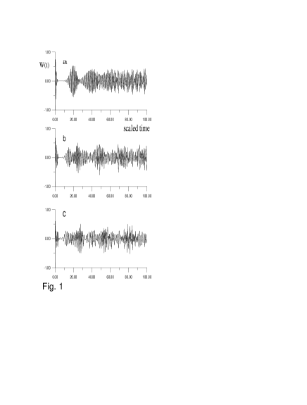
Figure 1: The atomic inversion $W(t)$ for the output field against the scaled time $\lambda t$. The values of the parameters are assumed as follows, the squeeze parameter $r=1$, the initial position (3,0), i.e $\alpha_{0}=3$, and the direction of squeeze is along the x-direction, i.e $\phi=0$. While the number of photons for the input state m takes different values, where (a) $m=0$, (b) $m=1$, and (c) $m=2$ .

We know that the collapses are caused by the dephasing of the various terms in the sums in equation (14). Thus we can calculate the time in which the revivals will occur by estimating the time that neighbor terms in the sums will be in phase again (for $n\sim\bar{n})$: $T_{R}(2\lambda\sqrt{\bar{n}+1}-2\lambda\sqrt{\bar{n}})\sim 2\pi.$ This argument is true in the case of coherent state and can be applied for the squeezed coherent state (i.e, $m=0$), as can be seen in figure 1a, but it cannot be applied for the SDFS. For nonzero m ($m=1$) figure 1b, not only the amplitude of Rabi oscillations, but also the time average of the inversion is affected. In figure 1c we have increased m to 2, and taken all other parameter as in figure 1a. One observes that for longer time the inversion shows small oscillations around zero but in quite irregular manner.

3.2 Entropy of the cavity field

Employing the reduced field density operator given by Eq. (12), we investigate the properties of the entropy. The quantum dynamics described by the Hamiltonian (6) leads to an entanglement between the field and the atom. We use the field entropy as a measurement of the degree of entanglement between the field and the atom of the system under consideration. In order to derive a calculation formalism of the field entropy, we must obtain the eigenvalues and eigenstates of the reduced field density operator given by Eq. (12). A general method to calculate the various field eigenstates in a simple way can be found in [4]. By using this method we obtain the eigenvalues and eigenstates of the reduced density operator,

$$\lambda_{f}^{\pm}(t)=\langle C(t)\mid C(t)\rangle\pm\exp[\mp\theta]\mid\langle C(t)\mid S(t)\rangle\mid$$ (15)

$$=\langle S(t)\mid S(t)\rangle\pm\exp[\pm\theta]\mid\langle C(t)\mid S(t)\rangle\mid,$$ (16)

$$\mid\psi_{f}^{\pm}(t)\rangle=\frac{1}{\sqrt{2\lambda_{f}^{\pm}(t)\cosh(\theta)}}\{\exp[(i\phi\pm\theta)/2]\mid C(t)\rangle$$ (17)

$$\pm\exp[-(i\phi\pm\theta)/2]\mid S(t)\rangle\},$$ (18)

where

$$\theta=\sinh^{-1}\biggl{(}\frac{\langle C(t)\mid C(t)\rangle-\langle S(t)\mid S(t)\rangle}{2\mid\langle C(t)\mid S(t)\rangle\mid}\biggr{)}.$$ (19)

We can express the field entropy $S_{f}(t)$ in terms of the eigenvalue $\lambda_{f}^{\pm}(t)$ of the reduced field density operator,

$$S_{f}(t)=-[\lambda_{f}^{+}(t)\ln\lambda_{f}^{+}(t)+\lambda_{f}^{-}(t)\ln\lambda_{f}^{-}(t)].$$ (20)

It does not appear possible to express the sums in equation (20) in closed form, but for not too large $\bar{n}$, direct numerical evaluation can be performed. On the basis of the analytical solution presented in the previous section, we shall examine the temporal evolution of the field entropy. It should be emphasized that in computing all infinite series for the atomic wave function $|\psi(t)\rangle$, we have invoked mathematically sound truncation criteria. To ensure an excellent accuracy the behavior of the field entropy function $S_{f}(t)$ has been determined with great precision. For regions exhibiting strong fluctuation a resolution of $10^{3}$ point per unit of time has been employed. The time t has been scaled; one unit of time is given by the inverse of the coupling constant $\lambda$.

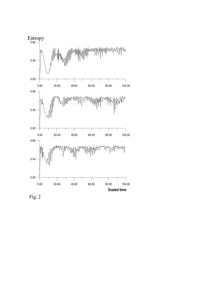
Figure 2: Entropy $S_{f}(t)$ of the output field against the scaled time $\lambda t$. The values of the parameters are assumed as follows, the squeeze parameter $r=1$, the initial position (3,0), i.e $\alpha_{0}=3$, and the direction of squeeze is along the x-direction, i.e $\phi=0$. While the number of photons for the input state m takes different values, where (a) $m=0$, (b) $m=1$, and (c) $m=2$ .

We display the evolution of the field entropy for different values of mean photon number $m$ and the squeeze parameter r is taken to equal $(r=1)$. In our computations, we have taken the displacement parameter $\alpha_{0}=3,\Delta=0$. In the case of an initial field with $r=0$ (coherent state), we already know [39-40] that the field evolves and (nearly) returns to a pure state only at half of the revival time. As further analysis showed, at that time the field is indeed in a superposition of coherent states. However, if we initially prepare the field in a squeezed state, as we see in figure 2, ($r=1$) that its entropy reaches a minimum at approximately the revival time corresponding to an initial coherent state with amplitude $\alpha$. Note that the revival time in the case of an initial squeezed state is $\lambda t=2\pi(\mid\alpha\mid^{2}+\sinh^{2}r)^{1/2}$. As we see in figure 2a, in the squeezed state case, the value of the entropy is almost the same at the revival time and at half of the revival time, and because they correspond to minima, the states of the field are less mixed at these times. However, near the minima the behavior of the entropy is different for the two cases. While the minimum is reached in a smooth way for the coherent state, it becomes oscillatory for the squeezed. The programme described near $S_{f}(t)$ has been carried out for several parameter sets, including those covered by figure 2. It may seem rather surprising to have a pure state at a time different from half of the revival time, but this is of course due to the nature of the squeezed states. Also, by increasing the squeezing parameter r, the field entropy becomes increasingly irregular and with values characteristic of a mixed state, $S_{F}(t)\simeq 0.7$. This is in qualitative agreement with the fact that the atomic response for the field initially prepared in a squeezed vacuum state is very similar to when it is prepared in a thermal (mixed) state [41]. To visualize the influence of SDFS in the field entropy we set different values of m $(m=1,2)$ and the squeeze parameter $r=1$, and all the other parameters are the same as in figure 2a. The outcome is presented in figure 2b, c. One can distinguish between two stages of evolution, each of which has been pictured separately. We see that the amplitude of the oscillations as well as the revival time becomes smaller and we have more revivals in the same time, the collapse time decreases. It is evident that the field and the atom are in the entangled state when m increases further. In next section we turn our attention to interesting non-classical phenomenon emerging as a direct consequence of quantum interference between component states of the field. Namely, we will analyse oscillations in the photon number distribution of the cavity field at different values of $m$.

3.3 Photon number distribution

In direct detection one counts the number of photons in the field mode of interest. The probabilty for finding $n$ photons: at time $t>0$, is given by

$$P(n,t)=|\langle n\mid\psi(t)\rangle|^{2}=\langle n|\rho_{f}(t)|n\rangle$$ (21)

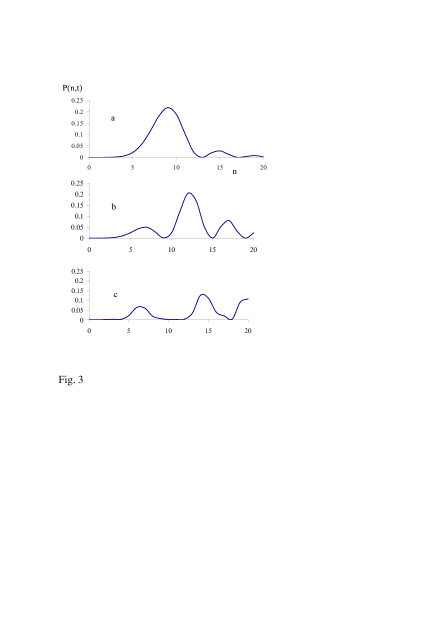
Figure 3: Plots for the photon number distribution $P(l,t)$ of the initial field. The values of the parameters are assumed as follows, the squeeze parameter $r=1$, the initial position (0.5,0), i.e $\alpha_{0}=0.5$, and the direction of squeeze is along the x-direction, i.e $\phi=0$. While the number of photons for the input state m takes different values, where (a) $m=0$, (b) $m=1$, and (c) $m=2$ .

from which we can easily find the photon number distribution of the cavity field in the one-photon JCM. As the cavity field starts to interact with the atom the initial photon number distribution $P_{n}=\mid q_{n}\mid^{2}$ starts to change. Due to the quantum interference between component states the oscillations in the cavity field become to be composed of two component states. Even though the field entropy is not equal to zero these two component states partially interfere which results in some oscillations of the photon number distribution. In figure 3 we plot the photon-number distribution of the cavity field in the case of nonzero squeezing parameter $r=1$ and for different values of m. We note that the amplitude of the photon-number distribution decreases as m increases see figure 3c (where we have set m=2). For $m=0$( figure 3a),the photon number distribution resembles a Poissonian distribution. In the large values of m, the amplitude of the oscillations is affected. As compared with the case $m=0$, the locations of the maxima have moved to the right as m increased further. For the entropy the characteristic sequence of minima is there again (figure 2c).

3.4 Phase distribution

Recently, Barnett and Pegg defined a Hermitian phase operator in a finite dimensional state space [34-36]. They used the fact that, in this state space, one can define phase states rigorously. The phase operator is then defined as the projection operator on the particular phase state multiplied by the corresponding value of the phase. The main idea of the Pegg-Barnett formalism consists in evaluation of all expectation values of physical variables in a finite dimensional Hilbert space. These give real numbers which depend parametrically on the dimension of the Hilbert space. Because a complete description of the harmonic oscillator involves an infinite number of states to be taken, a limit is taken only after the physical results are evaluated. This leads to proper limit which correspond to the results obtainable in ordinary quantum mechanics. It can be used for investigation of the phase properties of quantum states of the single mode of the electromagnetic field [34-37].

The Pegg-Barnett phase distribution $P(\eta)$ is defined through an infinite sum [34,35]:

$$P(\eta,t)=\frac{1}{2\pi}\sum_{l,j=0}^{\infty}\rho_{lj}(t)\exp[i(j-l)(\eta-\eta_{0})],$$ (22)

where the density matrix given by

$$\rho_{lj}(t)=(A_{l}(t)A^{*}_{j}(t)+B_{l-1}(t)B^{*}_{j-1}(t))$$ (23)

the angle $\eta_{0}$ is the phase reference angle and we take it to be zero. The phase distribution can be written as

$$P(\eta,t)=\frac{1}{2\pi}[1+2Re\sum_{j,l=0;j>l}^{\infty}\rho_{lj}(t)\exp[i(j-l)\eta]$$ (24)

We have computed the phase probability distribution function, related to a system of a 2-level atom in interaction with a single mode. In our computations, we have taken the displacement parameter $\alpha_{0}=3$, and the squeeze parameter $r=1$.

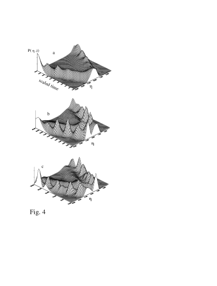
Figure 4: Shows the plot of phase distribution $P(\eta,t)$ as a function of the scaled time $\lambda t$ and $\eta$. The values of the parameters are assumed as follows, the squeeze parameter $r=1$, the initial position (3,0), i.e $\alpha_{0}=3$, and the direction of squeeze is along the x-direction, i.e $\phi=0$. While the number of photons for the input state m takes different values, where (a) $m=0$, (b) $m=1$, and (c) $m=2$.

Figure. (4) shows the time evolution of the phase probability distribution $P(\eta,t)$ for $r=1$ and for various values of $m$. When $m$ equal to zero, it is remarked that $P(\eta,t)$  exhibits symmetric splitting as $\lambda t$ varies as shown in figure (4a) This is the counterrotating behaviour observed earlier [37]. When $\lambda t=0$, $P(\eta,t)$ has a single-peak structure corresponding to the initial coherent state. The peaks are symmetric about $\eta=0$ so that the mean phase always remains equal to zero. The time behaviour of the phase probability distribution carries some information about the collapse and revival of Rabi oscillations [39]. When the phase peaks are well separated the Rabi oscillations collapse and each time as the peaks meet ( at $\eta=0$ and/or $\pm\pi$ ) they produce a revival see figure 4a. It is further noted that the height of the peak change as time develops in contrast to the case of the coherent input [39]. When $m\neq 0$, the situation is completely changed, as we observe from figure (4b-c). It is seen that when $m=1,$ thee are two peaks, one with small amplitude compared with the other peak, whose rate of shift becomes faster when plotted in a phase space as in [35]. It is observed that the symmetry shown in the the case when $m=0$ for the phase distribution is no longer present once the new state is added. The peaks are split but the two split peaks move with different rates. The one with the slower rate faces damping while the faster peak changes in the amplitude as time develops.

3.5 Evolution of the Q function

In the previous section we discussed a particular aspect of the atomic dynamics (collapses and revivals) in the one-photon model with the initial field prepared in the squeezed displaced Fock states. Now we are going to try to understand better the behaviour of the system by focusing our attention on the field dynamics by studing the quasi-distribution function. The first step to be taken is the calculation of the reduced density operator of the field $\hat{\rho}_{f}(t)$ (see equation (12)), we get for the Q function

$$Q(\alpha,t)=\frac{1}{\pi}\langle\alpha|\rho_{f}(t)|\alpha\rangle$$ (25)

where $|\alpha\rangle$ is a coherent state. More than just a theoretical curiosity, $Q(\alpha,t)$ can be detected in homodyne experiments [33] . It has the form

$$Q(\alpha,t)=\frac{1}{\pi}\exp(-|\alpha|^{2})\sum_{n,m=0}^{\infty}\rho_{nm}(t)\frac{(\alpha^{*})^{n}(\alpha)^{m}}{\sqrt{n!m!}}$$ (26)

The Q function is not only a convenient tool to calculate expectation values of anti-normally ordered products of operators, but also gives us a new insight into the mechanism of interaction in the model under consideration.

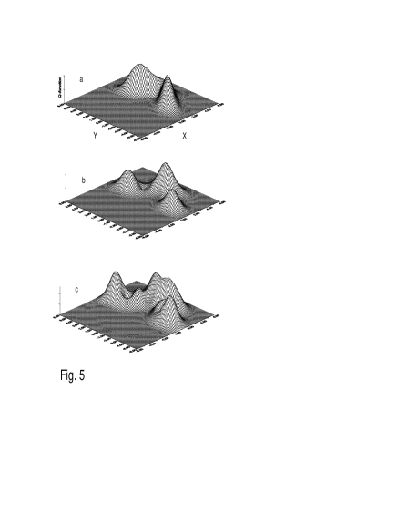
Figure 5: The Q function for the output of the JCM driven by the SDFS. The parameters are assumed as follows: The squeeze parameter $r=1$, $\phi=0$, $\alpha_{0}=3$, $\Delta=0$, and $m=1$. While the interaction time takes the values: (a) $t=0$; (b) $t=t_{R}/2$; (c) $t=t_{R}$. Here $X=Re(\alpha)$ and $Y=Im(\alpha)$.

In figure 5 we have sketched the Q-function distribution functions for the output field states. We here show this for the squeeze parameter $r=1$, $\alpha_{0}=3$, $m=1$ and for different values of the interaction time. We see that the Q function corresponding to the initial squeezed coherent state, [16], figure 5a bifurcates due to the quantum interaction between the field and the atom. At $\lambda t=0$ the Q function has a single-peak structure, but with $\lambda t=T_{R}/2$ we see that the Q function is composed of two well separated components, mean while if $\lambda t=T_{R}$, three components have been seen figure 5c. We show that at $t=0$ the peak of SDFS is observed [19]. For $t>0$ the two peaks split into two sets of counter-rotating peaks during the collapse. At longer times the Q-function is spread out over an angular region in the xy-plane as shown in figure 5. If we combine this observation with the fact that the field entropy at this moment is almost equal to zero we can conclude that the cavity field at $m=0$ is in a pure state. On the other hand at $m=1$ the entropy reaches its maximum and so in spite of fact that the Q function is composed of two parts the cavity field is in a statistical mixture state.

4 Summary and concluding remarks

The well-known Jaynes-Cummings Model gives an exactly solvable model of a two-level atomic system in interaction with a radiation field. We considered the interaction with the field initially is the SDFS. We have been studied in this work the three aspects, the first is the dynamics of the atomic inversion, the second is the field entropy, and later is the evolution of the output field statistics. The atomic inversion have discussed and plotted against the interaction time $\lambda t$. We found that it exhibited the conventional Rabi oscillation and collapse-revival for the SDFS. It is dependent on the parameters of the used state as squeeze parameter and number of photons. We further calculated the field entropy, which is zero for a pure state and non-zero for a mixed state. In general , for the atomic radiation system the field entropy was found to be non-zero. We have been considered the photon number distribution of the output field. We have been obtained the Pegg-Barnett phase distribution and also plotted with some parameters. The Q function for some parameters has presented analytically and numerically. The Q functin exhibited a variety of peaks with corresponding the photon number oscillation. Peak separation in the Pegg-Barnett phase distribution and the Q function is associated with the onset of the collapse and revivel of the atomic population inversion. The entropy is nearly zero when the Q function has exactly one peak, the greatest separation of Q function peaks corresponds to maximum entropy. The effects of squeeze parameter and photon number are obvious from all illustrations. The desire to realize physically certain specific quantum states such as SDFS’s is under current research. It is hoped that the SDF states will find applications in the quantum nondemolition measurements and quantum optics. They may also find application in experimental situations that require low noise sensitivity.

References

- [1] A. Caticha, Phys. Lett. A 244, 13 (1998); Phys. Rev. A 57, 1572 (1998)
- [2] S. J. D. Phoenix and P. L. Knight, Phys. Rev. A 44, 6023 (1991)
- [3] S. J. D. Phoenix and P. L. Knight, Phys. Rev. Lett. 66, 2833 (1991)
- [4] S. J. D. Phoenix and P. L. Knight, Ann. Phys. (N. Y) 186, 381 (1988)
- [5] J. Gea-Banacloche, Phys. Rev. Lett. 65, 3385 (1990); Phys. Rev. A 44, 5913 (1991); Opt. Commun. 88, 531 (1992)
- [6] M. Orszag, J. C. Retamal and C. Savedra, Phys. Rev. A 45, 2118 (1992)
- [7] P. Sarkar, S. Adhikari and S. P. Bhattacbaryya, Chem. Phys. 215, 309 (1997)
- [8] F. Farhadmotamed, A. J. van Wonderen and K. Lendi, J. Phys. A 31, 3395 (1998)
- [9] M. F. Fang and H. E. Liu, Phys. Lett. A 200, 250 (1995)
- [10] M. F. Fang and G. H. Zhou, Phys. Lett. A 184, 397 (1994)
- [11] M. F. Fang and X. Liu, Phys. Lett. A 210, 11 (1996)
- [12] R. J. Glauber, Phys. Rev. 131 2766 (1963)
- [13] J. Perina, Quantum statistics of linear and non-linear optical phenomena Reidel- Dordrecht, Holland (1984)
- [14] D. F. Walls and G. J. Milburn, Quantum Optics Springer-Verlag, Berlin (1994)
- [15] D. Stoler, Phys. Rev. D 1 3217 (1970); Phys. Rev. D 4 1925 (1970)
- [16] H. P. Yuen, Phys. Rev. A 13 2226 (1976)
- [17] R. Loudon and P. L. Knight, J. Mod. Opt. 34 709 (1987)
- [18] M. V. Satyanarayana, Phys. Rev. D 32 400 (1985)
- [19] P. Kral, J. Mod. Opt. 37 889 (1990); Phys. Rev. A 42 4177 (1990)
- [20] V. Perinova and J. Krepelka, Phys. Rev. A 48 3881 (1993)
- [21] A.-S. F. Obada, and G. M. Abd Al-Kader, J. Mod. Opt. 45 713 (1998); Nonlinear Opt. 19 143 (1998)
- [22] I. Foldesi, P. Adam, and J. Janszky, Phys. Lett. A 204 16 (1995)
- [23] Z. Z. Xin, Y.-B. Duan, H.-M. Zhang, M. Hirayama and K. Matumoto, J. Phys. B 29 4493 (1996)
- [24] K. B. Moller, T. G. Jorgensen, and J. P. Dahl, Phys. Rev. A 54 5378 (1996)
- [25] V. I. Man’ko and A. Wunsche, Quantum Semiclass. Opt. 9 381 (1997)
- [26] F. A. M. De Oliveira, M. S. Kim, P. L. Knight and V Buzek, Phys. Rev. A 41 2645 (1990)
- [27] N. Moya-Cessa and P. L. Knight, Phys. Rev. A 48 2479 (1993)
- [28] A. Wunsche, Quantum Opt. 3 359 (1991)
- [29] D. J. Wineland, C. Monroe, W. M. Itano, D. Leibfried, B. E. King, and D. M. Meekhof, J. Res. Natl. Inst. Stand. Technol. 103 259 (1998)
- [30] S.-B. Zheng and G.-C. Guo, Phys. Lett. A 244 512 (1998)
- [31] M. Dakna, L. Knöll and D.-G. Welsch, Eur. Phys. J. D 3 295 (1998)
- [32] K. E. Cahill and R. J. Glauber, Phys. Rev. 177s 1857, 1882 (1969); see the review M. Hillery, R. F. O’Connell, M. O. Scully and E. P. Wigner, Phys. Rep. 106 121 (1984) and references therein
- [33] H.-W. Lee, Phys. Rep. 259, 147 (1995)
- [34] S. M. Barnett and D. T. Pegg, J. Phys.A 19 3849 (1986)
- [35] S. M. Barnett and D. T. Pegg, Phys. Rev. A 39 1665 (1989); J. Mod. Optics 36 7 (1989)
- [36] R. Loudon, The quantum theory of light Clarendon Press. Oxford (1973)
- [37] Special issue on ” Quantum phase and phase dependent measurements” of Physica Scripta T48 s 1-142 (1993); R. Lynch, Phys. Rep. 256 367 (1995); V. Perinova, A. Luk and J. Peina, Phase in Optics World Scient, Singapore (1998)
- [38] S. Gradshteyn and I. M. Ryshik, Table of integrals, series, and products (Academic, New York (1980)
- [39] E. I. Aliskenderov and H. T. Dung, Phys. Lett. B 19 1279 (1993)
- [40] A.-S. F. Obada and M. Abdel-Aty, Acta Phys. Pol. B 31 589 (2000)
- [41] P. L. Knight and P. M. Radmore, Phys. Lett. A 90 432 (1982)