A magnetic model with a possible Chern-Simons phase

Abstract

An elementary family of local Hamiltonians $H_{\circ,\ell},\ell=1,2,3,\ldots$, is described for a $2-$dimensional quantum mechanical system of spin $=\frac{1}{2}$ particles. On the torus, the ground state space $G_{\circ,\ell}$ is $(\log)$ extensively degenerate but should collapse under $``$perturbation” to an anyonic system with a complete mathematical description: the quantum double of the $SO(3)-$Chern-Simons modular functor at $q=e^{2\pi i/\ell+2}$ which we call $DE\ell$. The Hamiltonian $H_{\circ,\ell}$ defines a quantum loop gas. We argue that for $\ell=1$ and $2$, $G_{\circ,\ell}$ is unstable and the collapse to $G_{\epsilon,\ell}\cong DE\ell$ can occur truly by perturbation. For $\ell\geq 3$, $G_{\circ,\ell}$ is stable and in this case finding $G_{\epsilon,\ell}\cong DE\ell$ must require either $\epsilon>\epsilon_{\ell}>0$, help from finite system size, surface roughening (see section 3), or some other trick, hence the initial use of quotes $``\quad$”. A hypothetical phase diagram is included in the introduction.

The effect of perturbation is studied algebraically: the ground state space $G_{\circ,\ell}$ of $H_{\circ,\ell}$ is described as a surface algebra and our ansatz is that perturbation should respect this structure yielding a perturbed ground state $G_{\epsilon,\ell}$ described by a quotient algebra. By classification, this implies $G_{\epsilon,\ell}\cong DE\ell$. The fundamental point is that nonlinear structures may be present on degenerate eigenspaces of an initial $H_{\circ}$ which constrain the possible effective action of a perturbation.

There is no reason to expect that a physical implementation of $G_{\epsilon,\ell}\cong DE\ell$ as an anyonic system would require the low temperatures and time asymmetry intrinsic to Fractional Quantum Hall Effect (FQHE) systems or rotating Bos$\acute{\textnormal{e}}$-Einstein condensates $-$ the currently known physical systems modelled by topological modular functors. A solid state realization of $DE3$, perhaps even one at a room temperature, might be found by building and studying systems, $``$quantum loop gases”, whose main term is $H_{\circ,3}$. This is a challenge for solid state physicists of the present decade. For $\ell\geq 3,\ell\neq 2\mod 4$, a physical implementation of $DE\ell$ would yield an inherently fault-tolerant universal quantum computer. But a warning must be posted, the theory at $\ell=2$ is not computationally universal and the first universal theory at $\ell=3$ seems somewhat harder to locate because of the stability of the corresponding loop gas. Does nature abhor a quantum computer?

0 Introduction

In section 1, we write down a positive semidefinite local Hamiltonian $H_{\circ,\ell}$ for a system of locally interacting Ising spins on a $2-$dimensional triangular lattice or surface triangulation, $\ell=1,2,3,\ldots$. In the presence of topology, e.g. on a torus, $H_{\circ,\ell}$ has a highly degenerate space $G_{\circ,\ell}$ of zero modes. On any closed surface $Y$, different from the $2-$sphere, the degeneracy is polylog $(2^{v})=$ poly$(v)$, where $v$ is the number of sites in the triangulation and the $2^{v}$ is the dimension of the Hilbert space $h$ of spins. On the torus $T^{2}$ the polynomial has degree $=1$, when $Y$ has genus $g>1$ the polynomial has degree $=3g-3$ (see Proposition 3.8).

We argue for an ansatz (3.4) which exploits the peculiarly rigid algebraic structure of $G_{\circ,\ell}\,\,-$ it is a monoidal tensor category with a unique nontrivial ideal. The ansatz allows us to model any $``$perturbed” ground state space $G_{\epsilon,\ell}$ (which is itself stable to perturbation) uniquely as a known anyonic system or in mathematical parlance a modular functor. The functor is the Drinfeld double of the even $-$ label $-$ sector of the $SU(2)$-Chern-Simons unitary topological modular functor at level $\ell,DE\ell$. Even labels corresponds in physical terms to the integer spin representations so the even-label-sector derives from the group $SO(3)$.

The Hamiltonian $H_{\circ,\ell}$ defines a quantum loop gas which can be compared (see Figure 3.12) with the classical analog. The statistical mechanics of classical loop gases [Ni] identifies a known critical regime and from this we infer that for $\ell=1$ and $2$, $G_{\circ,\ell}$ is unstable and the collapse to $G_{\epsilon,\ell}\cong DE\ell$ is truly by perturbation, for $\ell\geq 3,\,\,G_{\circ,\ell}$ is stable and in this case finding $G_{\epsilon,\ell}\cong DE\ell$ requires $\epsilon>\epsilon_{\ell}>0$, or some other device (see section 3), hence the initial use of quotes $``\quad$”. Figure 0.1 is a hypothetical phase diagram. The stability of $G_{\circ,\ell}$ at $\ell=3$ is probably very slight $-$ see footnote 6 in section 3 and the corresponding discussion.

The reader should not be alarmed that a $``$doubled” Chern-Simons theory arises. The doubled structure makes it a gauge theory and, as we will explain, the double, being achiral, is more likely to have a robust physical realization. The modular functor $DE\ell$ has $\lambda=\left(\lfloor\frac{\ell+1}{2}\rfloor\right)^{2}\,\,``$labels” or , physically, $\lambda$ super selection sectors for quasiparticle excitations (including the empty particle.) Physically this means that a local bit of material, a two dimensional disk with a fixed boundary condition, which is in its unique ground state $G_{\epsilon,\ell}$ can have $\lambda$ types of point-like anyonic excitations (presumably with exponentially decaying tails) which can only be created in pairs. $\lambda$ is the number of order integers pair $(x,y)$ with $0\leq x,y\leq\ell$, and $x,y=$ even. By mathematically deleting small neighborhoods of such excitations a ground state vector is approximately achieved in the highly degenerate ground state space $G_{\epsilon,\ell}$ associated to a punctured disk with boundary conditions. It is known [FLW2 ] and [FKLW] that for $\ell\geq 3,\ell\neq 0\mod 4$, there is a universal, inherently fault-tolerant, model for quantum computation based on the ability to create, braid, fuse, and finally distinguish these excitations types. Thus $H_{\circ,\ell}$ could be of technological importance: a physical system, a $``$quantum loop gas”, in this (perturbed) universality class could be the substrate of a universal fault tolerant quantum computer.

Any unit vector $\Psi\in G_{\circ,\ell}$ is a superposition of classical $\pm-$spin states $|\Psi\rangle$ which are distinguished by the eigenvalues $\pm 1$ of a commuting family of Pauli matrices $\sigma_{z}^{v}$ equal to $\left|\begin{smallmatrix}1&0\\ 0&-1\end{smallmatrix}\right|$ at vertex $v$. Sampling $\Psi=\SS a_{i}|\Psi_{i}\rangle$ by observing $\{\sigma_{z}^{v}\}$, we $``$observe” a classical $|\Psi_{i}\rangle$ with probability $|a_{i}|^{2}$. The domain wall $\gamma_{i}$ separating the $+$ - spin regions from ${-}$ - spin regions of $\Psi$ may be thought of as a random, self dual, loop gas [Ni]. This random state is self dual because there is a symmetry between $``$up” and $``$down”. It is a Gibbs state with parameters $k=0$, self dual, and $n=\left(2\cos\frac{\pi}{\ell+2}\right)^{2}$, where the weight of a configuration $\gamma$ is $w(\gamma)=e^{-k({\textnormal{total length }}\gamma)}n^{\#{\textnormal{ components }}\gamma}$. It is known that for $0<n\leq 2$ and $k=0$ the loop gas is critical, sitting at a $2^{\textnormal{nd}}$ order phase transition as $k$ crosses from negative to positive. This information together with sections $3$ or $4$ support a phase diagram like the one shown in Figure 0.1 with parameters $d:=2\cos\frac{\pi}{\ell+2}=\sqrt{n}$ and $\epsilon$. The parameter $\epsilon$ scales a local perturbation term $\epsilon V$. We will argue that the simplest choice for $V$, $V=\left(\underset{\textnormal{site }i}{\SS}\sigma_{x}^{i}\right)$, is a likely candidate. The diagram is labelled $``$hypothetical” since there is no proof of its accuracy.

The challenge to solid state physics is to find or engineer a two dimensional quantum medium in the universality class, $DE3$ below.

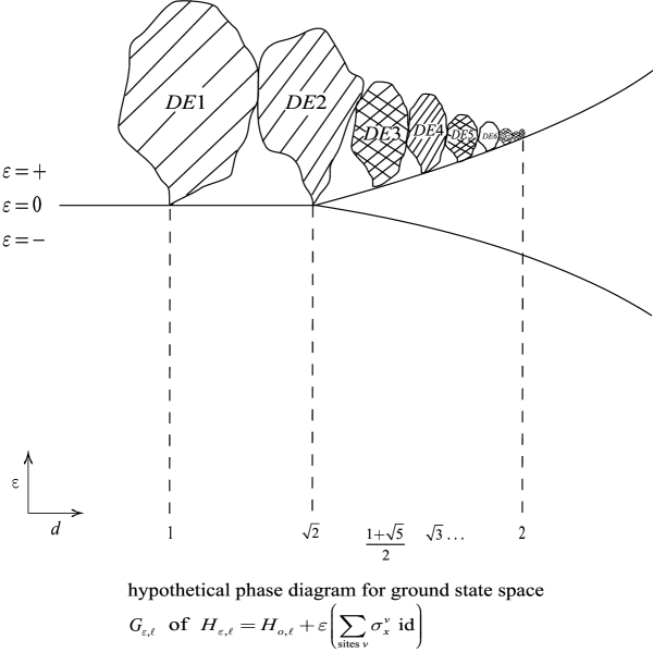
Figure 0.1: Shaded regions are the topological phases $DE1,DE2,DE3,DE4,\ldots$. Doubly shaded regions are the computationally universal phases $DE3,DE5,DE7,\ldots$. We have no way of predicting if the topological phases are actually in contact with each other as drawn. Solid lines are phase boundaries between inequivalent systems.

Theory	dim on $T^{2}$	number of constant color particles = labels and their braid reps.	number of additional color reversing particles and the total braid reps.	specific heat	nonsingular unitary topological modular functor? (UTMF)
DE1	1	1,T	1,T	2	yes, but trivially
DE2	4	4,T	1,N	5	no, rank $(S-\textnormal{matrix})=2$
DE3	4	4,U	4,U	8	yes
DE4	9	9,N	4,N	13	yes
DE5	9	9,U	9,U	18	yes
DE6	16	16,?	9,?	25	no
DE$\ell$	$\lceil\frac{\ell+1}{2}\rceil^{2}$	$\lceil\frac{\ell+1}{2}\rceil^{2}$, $U$ for $\ell\geq 5$, $\ell\neq 2\mod 4$	$\lceil\frac{\ell}{2}\rceil^{2}$, $U$ for $\ell\geq 5$, $\ell\neq 2\mod 4$	$\lceil\frac{(\ell+1)^{2}}{2}\rceil$	yes if $\ell\equiv 0,1,3\mod 4$ no if $\ell\equiv 2\mod 4$

Figure 0.2: For sufficiently many particles we have recorded if the (generalized) braid group representations are: T (trivial), A(abelian), N(nonabelian), U(computationally universal), we have called the total number of elementary particles, including those that reverse the $(|+\rangle,|-\rangle)$ coloring, $``$specific heat” as it counts local degrees of freedom above the ground state. The color constant elementary particles are the irreducible representations of the corresponding linear category (see $\S\,2$). Coloring-reversing particles are explained at the end of $\S\,2$.

The presumptive approach $-$ nearly universal in the literature $-$ to building a quantum computer is quite different from our topological/anyonic starting point. It is based on manipulating and protecting strictly local $-$ as opposed to global or topological $-$ degrees of freedom. It may be called the $``$qubit approach” since often a union of $2-$level systems (with state space $\underset{i}{\bigotimes}{\mathbb{C}}^{2}_{i}$) is proposed. Actually, the number of levels $-$ or even their finiteness $-$ is not the essential feature, it is that each tensor factor of the state space $-$ call it a qunit $-$ is physically localized in space (or momentum space). The environment will – despite the best efforts of the experimentalist $-$ interacted directly with these $``$raw” qunits. It has long been recognized ([S], [U]) that the raw qunits must encrypt fewer $``$logical qubits.” The demon in this approach is that very low initial (or raw) error rate - perhaps one error per $10^{-5}$ operations - and large ratios of raw to logical qunits $\sim 10^{3}$ seem to be required [Pr], to have a stable computational scheme. This problem pervades all approaches based on local or $``$qubit” systems: liquid NMR, solid state NMR, electron spin, quantum dot, optical cavity, ion trap, etc$\ldots$.

Kitaev’s seminal paper [K1] on anyonic computation, amplified in numerous private conversations, provides the foundation for the approach described here. Anyons are a $(2+1)-$dimensional phenomena: when sites containing identical particles in a $2-$dimensional system are exchanged (without collision) there are, up to deformation, two basic exchanges; a clockwise and a counter-clockwise half turn - or $``$braid” if the motion is considered as generating world lines in $2+1-$dimensional space-time. The two are inverse to each other but of infinite order rather than order $=2$. So whereas only the permutation needs to be recorded for exchanges in $R^{3}$, in $R^{2}$ $``$statistics” becomes a representation $\rho$ of a braid group $B$ into the unitary group of a Hilbert space $h$ encoding the internal degrees of freedom of the particle system:

$$\rho:B\longrightarrow U(h).$$

Since a representation into unitary transformations, $``$gate set” in (quantum) computer science language, is the heart of quantum computation it is not really a surprise that any kind of particle system with a sufficiently general (it certainly must be nonabelian) image $\rho(B)$ can be used to build a universal model for quantum computation. This has been shown in [FLW1], [FLW2], and [FKLW].

What are the advantages and disadvantages of anyonic verses qubit computation? The most glaring disadvantage of anyons is that no one is absolutely sure that nonabelian anyons exist in any physical system. Two dimensional electron liquids exhibiting the fractional quantum Hall effect FQHE are the most widely studied candidates for anyonic systems. The Laughlin state at filling fraction $\nu=1/3$ has observed excitations charges of $(1/3)e$ and these are convincingly linked by the mathematical model with a statistical factor of $\omega=\pm e^{2\pi i/3}$ for the exchange of such pairs. Quasiparticle excitations with nonabelian statistics is one of the most exciting predictions of Chern-Simons theory as a model for the FQHE. With a few low level (e.g. $\ell=1,2$ or $4$, when $G=SU(2)$) exceptions nonabelian anyonic systems are capable, under braiding, of realizing universal quantum computation [FLW2]. The essential point is that the $``$Jones representation” of the braid group (on sufficiently many strands) associated to the Lie group $SU(2)$ has a dense image at least in $SU(h)\subset U(h)$, $h$ an irreducible summand of the representation. At $\nu=5/2$ according to [RR] the Hall fluid is modelled by a $U(1)$ theory coupled to CS$2$ [the Chern-Simons theory of $SU(2)$ at the $4^{\textnormal{th}}$ root of unity (level $\ell=2$)]; the latter is a theory with a nonabelian $``$Clifford group” representation. This model was selected from conformal field theories to match expected ground state degeneracies and central charge, and is further supported by numerical evidence on the overlap of trial wave functions. Though very interesting, this representation is still discrete and is not universal in the sense of [FLW1]. However at $\nu=8/5$, with perhaps weaker numerical support [RR], it is thought that the Hall fluid model contains by $CS3$ (level$=3$, $5^{\textnormal{th}}$ root of unity). Here braiding and fusing the excitation would yield universal quantum computation [FLW1].

So let us, for the sake of discussion, accept that FQHE systems have computationally universal anyons, we are still a long way from building a quantum computer. FQHE systems are very delicate:

1. The required crystals have been grown successfully only in a few laboratories.

2. The temperatures at which the finer plateaus are stable are order milK.

3. The chiral asymmetry intrinsic (For CS2 and CS3 the central charge is $\frac{3}{2}$ and $\frac{9}{5}$ respectively.) to the effect requires an enormous transverse magnetic field, order 10 - 15 Tesla to reduce magnetic length to where conduction plateaus are observed.

At feasible magnet lengths, the Coulomb interaction between electrons is at least three orders of magnitude weaker than in solids. Corresponding to the weakness of these interactions the spectral gap protecting topological phases is necessarily quite small. Perhaps for this reason, even the most basic experiments to prove existence of $``$nonabelions” have not been carried out, and the use of these systems for computations appears unrealistic.

For applications such as breaking the cryptographic scheme RSA, it can be estimated that several thousand anyons must be formed, braided at will (perhaps implementing tens of thousands of half twists), and finally fused. This appears to be a nearly impossible task in a FQHE system.

The main point of this paper is that computationally universal anyons may be available in more convenient systems. $H_{\circ,\ell}$ is a local model for a paramagnetic system of Ising spins with short range antiferromagnetic properties. Written out in products of Pauli matrices $H_{\circ,\ell}$ is seventh order (on the standard triangular lattice) and thus looks complicated compared to, say, the Heisenberg magnet. But geometrically it is quite simple and its ground states are known exactly. A $2-$dimensional material in the universality class $DE\ell$ proposed as the ground state space for $H_{\epsilon,\ell},\ell\neq 1,2,$ or $\equiv 0\mod 4$, will have excitations - $``$quasiparticles” - capable of universal fault tolerant quantum computation within a model that allows creation, braiding, fusion and measurement of quasiparticle type.

A topological feature is not too easy to detect; by definition, topological properties cannot be altered or measured by purely local operators but instead require something akin to an Aharonov-Bohm holonomy experiment. So perhaps the universality class of $H_{\epsilon,\ell}$ already exists in surface layer physics but is waiting to be discovered. Or perhaps with $H_{\circ,\ell}$ in mind something in its (perturbed) universality class can be engineered. If this is possible there would be no reason to expect the system to be particularly delicate. The characteristic energies for magnets are often several hundred Kelvin [NS]. Furthermore the modular functor $DE\ell$ (this includes the information of the various braid group representations, $6_{j}-$ symbols, $S$ and fusion matrices) which arises is amphichiral, the central charge $c=0$, so there is no reason that time symmetry must be broken and no apparent need for a strong transverse magnetic field. These two features are in marked contrast to the delicate FQHE systems.

Subsequent to the initial draft of this paper a different local Hamiltonian $H^{\prime}_{\circ,\ell}$ was found which bears the same relation as $H_{\circ,\ell}$ to the topological modular functors $DE\ell$, but has potential advantages:

1. it is expressible as $4^{\textnormal{th}}$ rather than $7^{\textnormal{th}}$ order interactions and
   

2. its classical analog is the much studied self dual Potts model for $q=\left(2\cos\frac{\pi}{\ell+2}\right)^{4}$.

We have added a section $1^{\prime}$ following section 1 to explain this alternative microscopic model.

We make no proposal here for a specific implementation of $H_{\circ,\ell}$ or for how to trap and braid its excitations but we hope that models in the spirit of [NS] for the high $T_{c}$ cuprates may soon be proposed. In this regard, we note that relatively simple - but still non classical-braiding statics have been proposed [SF] in conjunction with the phenomena of spin-charge separation [A] for high $T_{c}$ cuprate super conductors above their $T_{c}$. Certain $-1$ phases are predicted to occur when braiding the electron fragments $``$visions” and $``$chargeons” around each other and around ground state defects called $``$holons”. Also contained in this paper is the suggestion that topological charges might in passing though a phase transition become classical observables, e.g. magnetic vortices. Similarly other phase transitions might link higher $(\ell=3)$ to lower $(\ell=1)$ topological phases and might be useful in measuring quasiparticle types. Whether even the simplest topological theory is realized in any known superconductor is open, but [SF] is cited as precedent for anyonic models for solid state magnetic systems with high characteristic energies. So while the FQHE motivates this paper, we hope we have steered toward its mathematical beauty and away from it experimental difficulties.

What are the generic advantages of anyonic computation? First information is stored in topological properties $``$large scale entanglement” of the system that cannot be altered (or read) by local interaction. This affords a kind of physical stability against error rather than the kind of combinatorial error correction scheme envisioned in the qubit models - $``$hardware” rather than $``$software” error correction. Second, at least in the simplest analysis, one expects excitation of a stable system to be well localized with exponentially decaying tails. Thus physical braiding should approximate mathematical braiding, $\rho:B\longrightarrow U(h)$ up to a $``$tunnelling” error of the form $e^{-cL}$, where $c$ is a positive constant, and $L$ is a microscopic length scale describing how well separated the excitations are kept during the braiding process. This error scaling is highly desirable and seems to have no analog in qubit models. While tunnelling treats virtual errors, errors which borrow energy briefly from the vacuum, actual errors would be expected scale like $e^{-c_{1}T/T_{\circ}}$ where $T_{\circ}$ is a character energy for the system and $T$ the operating temperature. This is essentially the error analysis Kitaev made for his anyonic system, the toric code [K1].

This paper draws on three sources of inspiration: 1) Kitaev’s paper [K1] on anyonic computation, 2) the FQHE, and 3) rigidity in the classification of von Neumann algebras subfactors. Rigidity implies that certain monoidal tensor categories have very few ideals. But when interpreted physically, $``$ideal” means $``$definable by local conditions”, so we find that a certain locality assumption (Ansatz 3.4) strongly limits the physics. This provides an algebraic approach to the perturbation theory of $H_{\circ,\ell}$ - and perhaps yields greater insight than would be possible by analytic methods. We find that for $H_{\circ,\ell}$ the polylog extensively degenerate space of $0-$modes $G_{\circ,\ell}$ possess in addition to its linear structure, an important $``$multiplicative” structure $-$ the structure of a monoidal tensor category - which we argue, should be preserved under a perturbation. The rigidity of type II<sub>1</sub> factor pairs, an aspect of which is stated as Thm 2.1, provides a unique candidate for the (still finitely degenerate) $``$perturbed” ground state space $G_{\epsilon,\ell}$ of $H_{\epsilon,\ell}$. The space $G_{\epsilon,\ell}$ is a braid group representation space with the representation induced by an adiabatic motion of quasiparticle excitations.

Throughout, the excitations on a surface $Y$ are assumed to be localized near points so excited states of $H_{\epsilon,\ell}(Y)$ become ground states of $H_{\epsilon,\ell}(Y^{-})$ but now on a punctured surface $Y^{-}$ with $``$boundary conditions” or more exactly $``$labels,” (see section 2.) We treat excited states indirectly as ground states on the more complicated surface $Y^{-}$.

The existence of a stable phase $G_{\epsilon,\ell}\cong DE\ell$ will be argued by analogy with the FQHE where topological phases are found to be stable, from algebraic uniqueness, and via $``$consistency checks”. But these arguments constitute neither a mathematical proof nor a numerical verification. The latter may be exactly as far off as a working quantum computer. It was precisely the problem of studying quantum mechanical Hamiltonians in the thermodynamic limit, e.g. questions of spectral gap, that lead Feynmann [Fe] to dream of the quantum computer in the first place. It is curiously self-referential that we may need a quantum computer to $``$prove” numerically that a given physical system works like one.

We turn now to the definition of $H_{\circ,\ell}$ and $H^{\prime}_{\circ,\ell}$; returning later to amplify on the relations to quantum computing, ${\mathbb{C}}^{\ast}-$ algebras, Chern-Simons theory, and topology. (The connection between Chern-Simons Theory and complexity classes is discussed in [F1].)

In addition to Alexei Kitaev, I would like to thank Christian Borgs, Jennifer Chayes, Chetan Nayak, Oded Schramm, Kevin Walker, and Zhenghan Wang for stimulating conversations on the proposed model.

1 The model

The model describes a system of spin $=\frac{1}{2}$ particles located at the vertices $v$ of a triangulated surface $Y$. The Hilbert space is $\mathcal{H}={\underset{v=1}{\overset{n}{\bigotimes}}}{\mathbb{C}}^{2}_{v}$ where ${\mathbb{C}}^{2}_{v}$ is the local degree of freedom $\{\mid+\rangle,\mid-\rangle\}$ at the vertex $v$. The basic Hamiltonian $H_{\circ,\ell}$ is written out below as a sum of local projections and thus is positive semidefinite. The ground state space (energy $=0$ vectors) $G_{\circ,\ell}$ of $H_{\circ,\ell}$ can be completely understood (this is unusual since the projector above do not commute) and identified (as $n\longrightarrow\infty$) with what we call the even Temperley-Lieb surface $``$algebra” ${\textnormal{ETL}}^{s}_{d}$ where $d=2\cos\frac{\pi}{\ell+2}$.

Ultimately our focus will be on the ground states on a multiply punctured disk $-$ the puncture corresponding to anyonic excitations (see section 5). Two issues arise: (1) non-trivial topology and (2) boundary conditions. The boundary conditions are quite tricky so it is best to work first with closed surfaces of arbitrary genus (even though these are not our chief interest) to understand the influence to topology alone $``$liberated” from boundary conditions.

$Y$ will denote a compact oriented surface throughout. In combinatorial contexts, $Y$ will be given a triangulation $\triangle$ with dual cellulation $\mathcal{C}$. Initially, we consider the case where $Y$ is closed, boundary $Y=\partial Y=\emptyset$. We will speak in terms of the dual cellulation by $2-$cells or $``$plaques” $c$. For example, if $Y$ is a torus it may be cellulated with regular hexagons. This is a perfectly good example to keep in mind but higher genus surfaces are also interesting, while the sphere is less so. Soon we will consider surfaces with boundary.

Distributing $\bigotimes$ over $\bigoplus$, one writes $\mathcal{H}=$ span $\{$classical spin configurations on plaques$\}=:$ span $\{s_{i}\}$. Let $c$ be a plaquet, $s$ a classical spin configuration and $\overline{s}^{c}$ that configuration with reversed spin $(+\longrightarrow-$ and $-\longrightarrow+)$ at $c$. For $1<i,j\leq 2^{n}$ define $h_{ij}(c)=1$ if $(1)s_{j}=\overline{s}_{i}^{c}$ and $(2)s_{i}$ assigns the same spin $\pm$ to $c$ and all its immediate neighbors, and $h_{ij}(c)=0$ otherwise. Define $g_{ij}(c)=1$ if $(1)s_{j}=\overline{s}^{c}_{i}$ and (2) the domain wall $\gamma_{s_{i}}$ between $+$ and $-$ plaques, in the spin configuration $s_{i}$, meets $c$ in a single connected topological arc, and $g_{ij}(c)=0$ otherwise. We define:

$$H_{\circ,\ell}= \sum_{\begin{subarray}{1}\textnormal{plaques $c$, pairs}\\ \textnormal{of spin states }s_{i},s_{j}\end{subarray}}g_{ij}(c)\left(\left(|s_{i}\rangle-|s_{j}\rangle\right)\left(\langle s_{i}|-\langle s_{j}|\right)\right)+$$ (1.1)

$$\kappa \sum_{\begin{subarray}{1}\textnormal{plaques $c$, pairs}\\ \textnormal{of spin states }s_{i},s_{j}\end{subarray}}h_{ij}(c)\left(\left(|s_{i}\rangle-\frac{1}{d}|s_{j}\rangle\right)\left(\langle s_{i}|-\frac{1}{d}\langle s_{j}|\right)\right)$$

The constant $\kappa$ is positive and may, in this paper, be set as $\kappa=1$. To help digest the notation each of the two sums has $n2^{2n}$ terms most of which are zero. It is easy to see that $g_{ij}=g_{ji}$. If the domain wall $\gamma$ meets $c$ in a topological arc reversing the spin of $c$ isotopes the domain wall across $c$ to the complementary arc $=\overline{\partial c\smallsetminus\gamma}$. Contrariwise if $h_{ij}=1$ then $h_{ji}=0$. The parameter ${d}$ could be any positive real number but we will be concerned mainly with $d=2\cos\frac{\pi}{\ell+2},\ell=1,2,3,\cdots$. The cases $\ell=2$, $d=\sqrt{2}$ and $\ell=3$, $d=\frac{1+\sqrt{5}}{2}$, the golden ratio, are of particular interest. Finally, each term in the definition of $H_{\circ,\ell}$ should be read, according to the usual ket-bra notation, as orthogonal projection onto the indicated vector: $|s_{i}\rangle-|s_{j}\rangle$ or $|s_{i}\rangle-1/d\,|s_{j}\rangle$. These vectors (whose projectors occur nontrivially in the sums) are certainly not orthogonal to each other (using the inner product $|+\rangle$ hermitian orthonormal to $|-\rangle$ in ${\mathbb{C}}^{2}$, extended to define the tensor product Hermitian structure on $\mathcal{H}$) so those individual projectors do not commute. It is therefore surprising at first that we can completely describe the (space of) zero modes $G_{\circ,\ell}$ of this positive semidefinite form, $H_{\circ,\ell}$. However once the description is given the surprise will evaporate for it will be clear how $H_{\circ,\ell}$ was $``$engineered” precisely to yield this result. Identifying $G_{\circ,\ell}$ is the next goal.

Associate to the closed oriented surface $Y$ an infinite dimensional vector space ETL${}_{d}(Y)$, the even Temperley-Lieb space of $Y$. It is the ${\mathbb{C}}-$span of $``$isotopy classes” of closed bounding $1-$ manifolds $\gamma$ modulo a relation called $d-$isotopy. The $``$bounding” condition means that $\gamma$ is a domain wall separating $Y$ into two regions which could be labelled $``|+\rangle$” and a $``|-\rangle$”. Neither $\gamma$ nor the regions are presumed to be connected. We do not orient $\gamma$, so we do not distinguish here between states which differ by globally interchanging $|+\rangle$ and $|-\rangle$. The term $``1-$manifold” means $\gamma$ does not branch or terminate at any point. Isotopy, of course, means gradual deformation. The $d-$isotopy relation: $\gamma-d(\gamma\setminus\gamma_{\circ})$, when imposed, says that if a component $\gamma_{\circ}$ of $\gamma$ bonds a disk in $Y$ then $\gamma=d(\gamma\setminus\gamma_{\circ})$, $d$ times the value on the submanifold with $\gamma_{\circ}$ deleted. We often work with the dual $ETL^{\ast}_{d}(Y)$, which are the functions $f$ on bounding isotopy classes satisfying $f(\gamma)=d(f(\gamma\setminus\gamma_{\circ}))$. Let $\gamma^{!}$ be a $\gamma$ as above enhanced by one of the two choices for $``$signing” the complementary regions. Define $ELT^{!}_{d}(Y)$ to be ${\mathbb{C}}-$span $\{\gamma^{!}\}$, so that $ELT^{!\ast}_{d}(Y)$ are the functions from $\{\gamma^{!}\}$ obeying the $d-$isotopy relation.

Both the definition of $H_{\circ,\ell}$ and $ETL^{\ast}_{d}$ can easily be extended to $Y$ a compact surface with boundary $=\partial Y$, given a fixed boundary condition, the points where $\gamma$ meets $\partial Y$ (transversely). So if $\triangle$ is a triangulation of $(Y,\partial Y)$ with dual cellulation $\mathcal{C}$ and if the spin configuration $|+\rangle$ or $|-\rangle$ is fixed at every vertex ($=$ dual cell) on $\partial Y$ then formula (1.1) defines a Hamiltonian operator on the configurations with that boundary condition provided, in both terms, we restrict the sum to plaques $c$ which do not meet $\partial Y$. This prevents $``$fluctuations” from altering the boundary conditions. Define $H_{\circ,\ell}(Y,\partial Y)$ in this way. Similarly if a $2-$coloring (or $+$, $-\,``$signing”) of $Y$ is fixed along $\partial Y$ we may consider a relative $\gamma^{!}$ as a extension of this signing to a division of $Y$ into $+$ and $-$ signed regions (which are presumed to lie in $Y$ as subsurfaces). Now relative to the boundary condition (the signing) $ETL^{!\ast}_{d}(Y,\partial Y)$ is defined as functions from $\{\gamma^{!}\}$ to ${\mathbb{C}}$ which obey the $d-$ isotopy relation; $ETL^{\ast}_{d}(Y,\partial Y)$ is the set of such function invariant under ^-, the global $|+\rangle\longleftrightarrow|-\rangle$ interchange.

If $\triangle$ is a triangulation on a surface $Y$, with or without boundary then we have the combinatorial versions of ETL${}_{d}^{!}(Y)$ and ETL${}_{d}(Y)$, ETL${}^{\triangle!}_{d}(Y)$ and ETL${}^{\triangle}_{d}(Y)$ (resp.) define using only $(|+\rangle,|-\rangle)2-$colorings in which each dual $2-$cell (plaquet) is $+$ or $-$.

There are natural maps of ${\mathbb{C}}-$vector spaces:

$$\textnormal{ETL}^{\triangle!}_{d}(Y)\rightarrow\textnormal{ETL}^{!}_{d}(Y)\textnormal{ and }\textnormal{ETL}^{\triangle}_{d}(Y)\rightarrow\textnormal{ETL}_{d}(Y).$$ (1.2)

These maps are of course never onto (only the simpler $d-$isotopy classes are realized). Also for certain triangulations $\triangle$ the kernel can also be non-zero (due to $``$stuck” configurations). However, it is easy to see that as $\triangle$ is subdivided. $ETL^{\triangle}_{d}(Y)$ approximates $ETL_{d}(Y)$ in the sense that the direct limit $\underrightarrow{\lim}\,ETL^{\triangle}_{d}(Y)\cong ETL_{d}(Y)$, similarly $\underrightarrow{\lim}\,ETL^{\triangle!}_{d}(Y)\cong ETL^{!}_{d}(Y)$.

Let $\triangle$ be a fixed triangulation of $Y$ (with fixed boundary condition $-$ a ${}^{-}\,\,-$ projective $(|+\rangle,|-\rangle)\,2-$coloring $-$ if $\partial Y\neq\emptyset$), set $G_{\circ,\ell}(Y,\triangle)=$ zero modes (ground state space) of the positive semidefinate $H_{\circ,\ell}$ defined above (1.1). Clearly $H_{\circ,\ell}$ is ${}^{-}-$invariant and so $G_{\circ,\ell}$ is ${}^{-}-$invariant. Note that ^- is not always fixed point free: on $Y=T^{2}$, the configuration which is $|+\rangle$ on an essential annulus $A\subset T^{2}$ and $|-\rangle$ on $T^{2}\smallsetminus A$ is a ${}^{-}\,\,-$ fixed point. Let $G_{\circ,\ell}^{+}(Y,\triangle)$ denote the $+1-$eigenspace of ^-.

Proposition 1.1.

For $Y$ a closed surface or a surface with fixed boundary conditions, there are natural isomorphisms $G_{\circ,\ell}(Y,\triangle)\cong\textnormal{ETL}^{\triangle!}_{d}(Y)\textnormal{ and }G_{\circ,\ell}^{+}(Y,\triangle)\cong\textnormal{ETL}^{\triangle}_{d}(Y)$.

Proof: From line (1.1), $\Psi\in G_{\circ}(Y,\triangle)$ iff $\Psi=\underset{i}{\SS}(f|s_{i}\rangle)|s_{i}\rangle$ for some linear functional obeying the $d-$isoptopy relation, thus $G_{\circ,\ell}(Y,\triangle)\cong\textnormal{ETL}^{\triangle!}_{d}(Y)$. The involution ^- acts compatibility on both sides so $\textnormal{ETL}^{\triangle}_{d}(Y)$ may be identified as the $+1$ eigenspace of ^- on the r.h.s. ∎

When we come (section 3) to imposing the mathematical structure of a modular functor (or TQFT) on the ground state spaces $G^{+}_{\circ,\ell}(Y)$ for various surfaces $Y$ we will need to impose a base point $\ast$ on each boundary component $C\subset\partial Y$. This is directly analogous to the framing of Wilson loop in [Wi], in fact the base point moving in time defines the first direction of a normal frame to the Wilson loop in the $2+1$ dimensional space-time picture. As in the previous application, the base point is introduced for mathematical rather than physical reasons. It allows the state vectors in each conformal block to be identified precisely and not merely up to a (block-dependent) phase ambiguity. Concretely in our model the base point prevents domain walls from spinning around a puncture. Note that if (a superposition of) domain walls $\gamma$ represent an eigenspace for Dehn twist around the puncture with eigenvalue $\lambda\neq 1$ and if twisting is not prevented then the relation $|\gamma\rangle=\lambda|\gamma\rangle$ will occur, killing the state $|\gamma\rangle$ which is certainly not desired. I thank Nayak for pointing out that although choosing base points breaks symmetry, none of the physics depends on which base points are chosen. The Hamiltonian has a $\underset{k}{{\underbrace{U(1)\times\cdots\times U(1)}}}-$gauge symmetry where $k=\#$ boundary components of $Y$.

$\bf 1^{\prime}$ An alternative microscopic model.

In this subsection we present an alternative Hamiltonian, $H^{\prime}_{\circ,\ell}$, on a cellulated surface $(Y,\mathcal{C})$. We do not restrict to triangulation since the square lattice actually yields the simplest form. It has the same relation, in the infrared, to topological theories as does $H_{\circ,\ell}$. In this model the degrees of freedom are on bonds and the loops lie in a $``$midlattice” separating the $|+\rangle$ clusters from the $|-\rangle$ dual clusters (isolated vertices and isolated dual vertices count as clusters). There are perhaps three advantages:

1. On a square lattice, all terms in the Hamiltonian have order $4$ (as compared to seven in the previous model). It is simple enough that we expand it as a product of Pauli matrices.
   

2. The corresponding classical statistical mechanical model is the Potts model in cluster expansion $(FK)$ form with $q=(2\cos\frac{\pi}{\ell+2})^{4}$.; and
   

3. The loops in this model are $``$fully packed” so no isotopy is possible, only $d-$isotopy. In particular the total length of the loops separating $|+\rangle$ from $|-\rangle$ is configuration independent. Here is $H^{\prime}_{\circ,\ell}$ ; the notation is explained below.

$$\begin{split}H^{\prime}_{\circ,\ell}=&\sum_{\includegraphics[width=7.11317pt,height=7.11317pt]{drawingb.eps}}\left(|3\rangle-\frac{1}{d}\,|4\rangle\right)\left(\langle 3|-\frac{1}{d}\langle 4|\right)+\\ &\kappa\,\,\sum_{\includegraphics[width=7.11317pt,height=7.11317pt]{drawingc.eps}}\left(|\widehat{1}\rangle-\frac{1}{d}|\widehat{0}\rangle\right)\left(\langle\widehat{1}|-\frac{1}{d}\langle\widehat{0}|\right)\end{split}$$ (1.3)

$\kappa$ is a positive constant which for symmetry we suppose to be $\kappa=1$. Again $d=2\cos\frac{\pi}{\ell+2}$. On each bond there is a spin $=\frac{1}{2}$ degree of freedom $={\mathbb{C}}^{2}=$ span $\{|+\rangle,|-\rangle\}$. The first summation is over all plaques ($2-$ cells) with a market edge (So, if the surface is a $10\times 10$ torus cellulated with $100$ squares, the first summand contains $400$ terms.) Each term in the first sum is orthogonal projection onto the vector $\left(|-\rangle\otimes|+\rangle\otimes|+\rangle\otimes\dots\otimes|+\rangle-\frac{1}{d}|+\rangle\otimes|+\rangle\otimes|+\rangle\otimes\dots\otimes|+\rangle\right)$ where the tensor factors begin with the bond containing the dot and proceed counterclockwise around the plaquet. (Of course this projector is understood to be tensored with the identity over all remaining bonds.) Perhaps this is confusing, but we have used the notation $|3\rangle$ for the first and $|4\rangle$ for the second basis vector in this combination because in the square lattice case, those numbers count the $+$ signs: a more elaborate notation would be $|n_{i}-1\rangle-\frac{1}{d}|n_{i}\rangle$. The second term is the $``$double dual” of the first where one duality swaps cellulation with dual cellulation (homology with cohomology) and the other duality swaps $|+\rangle$ and $|-\rangle$. Thus the second summation is over vertices with a marked incoming bond; the vector $|\widehat{1}\rangle$ denotes $|+\rangle\otimes|-\rangle\otimes|-\rangle\otimes\dots\otimes|-\rangle$ and $|\widehat{0}\rangle$ denotes $|-\rangle\otimes|-\rangle\otimes|-\rangle\otimes\dots\otimes|-\rangle$, again reading counterclockwise from the dot. The ^∧ reminds us that we are reading around a site not a plaquet. In the case of the square lattice the two types of terms may be expressed as a $4^{\textnormal{th}}$ degree polynomial in Pauli matrices: $\sigma_{z}=\begin{smallmatrix}{}_{|+\rangle}\\ {}_{|-\rangle}\end{smallmatrix}\overset{\begin{smallmatrix}{}_{|+\rangle}&{}_{|-\rangle}\end{smallmatrix}}{\left|{\begin{smallmatrix}{1}&{\,\,\,0}\\ {0}&{-1}\end{smallmatrix}}\right|}$ and $\sigma_{x}=\left|\begin{smallmatrix}{0}&{1}\\ {1}&{0}\end{smallmatrix}\right|$.

$H^{\prime}_{\circ,\ell}$ has two types of terms:

$$= \left[\frac{1}{16}(I-\sigma^{0}_{z})-\frac{1}{8d}\sigma^{0}_{x}+\frac{1}{16d^{2}}(I+\sigma^{0}_{z})\right]\otimes\left[(I+\sigma^{1}_{z})\otimes(I+\sigma^{2}_{z})\otimes(I+\sigma^{3}_{z})\right],\textnormal{ and}$$

$$\left[\frac{1}{16}(I-\sigma^{0}_{z})-\frac{1}{8d}\sigma^{0}_{x}+\frac{1}{16d^{2}}(I+\sigma^{0}_{z})\right]\otimes\left[(I-\sigma^{1}_{z})\otimes(I-\sigma^{2}_{z})\otimes(I-\sigma^{3}_{z})\right]$$

$$= \frac{1}{16}\left[\frac{d^{2}+1}{d^{2}}I+\frac{1-d^{2}}{d^{2}}\sigma^{0}_{z}-\frac{2}{d^{2}}\sigma^{0}_{x})\right]\otimes\left[(I+\sigma^{1}_{z})\otimes(I+\sigma^{2}_{z})\otimes(I+\sigma^{3}_{z})\right],\textnormal{ and}$$

$$\frac{1}{16}\left[\frac{d^{2}+1}{d^{2}}I+\frac{d^{2}-1}{d^{2}}\sigma^{0}_{z}-\frac{2}{d^{2}}\sigma^{0}_{x}\right]\otimes\left[(I-\sigma^{1}_{z})\otimes(I-\sigma^{2}_{z})\otimes(I-\sigma^{3}_{z})\right]$$

The proper context for understanding $H^{\prime}_{\circ,\ell}$ is Baxter’s $``$mid lattice” [B]. If $\mathcal{C},\mathcal{C}^{\ast}$ are cellulation and dual cellulation, let $c^{\prime}=c\cap c^{\ast}$ be the general intersection of a plaquet and a dual plaquet. Put a center $\ast$ in $c^{\prime}$ and a center point $\ast_{1},\dots\ast_{n}$ in each of its boundary $1-$ cells. Subdivide $c^{\prime}$ by the cone of $\underset{i=1}{\overset{n}{\bigcup}}\ast_{i}$ to $\ast$ and let $c^{\prime\prime}$ denote the general plaquet of this subdivision. The collection $\{c^{\prime\prime}\}$ are precisely the plaquets of the $``$mid lattice”. As an example, for the square lattice of unit size the dual lattice is shifted by $(1/2,1/2)$ and the resulting mid lattice is spanned by vectors $\{(0,1/4),(1/4,0)\}$.

A classical configuration $s:\{\textnormal{bonds of }\mathcal{C}\}\longrightarrow\{|+\rangle,|-\rangle\}$ is encoded as the union of bonds on which $s$ is $|+\rangle$, the components of which are called clusters and the union of the duals of bonds on which $s$ is $|-\rangle$, whose components are called dual clusters. There is a well defined $1-$ manifold (multi$-$loop) $\gamma_{s}$ in the mid lattice which separates clusters from dual clusters.

The Hamiltonian $H^{\prime}_{\ell,\circ}$ builds in dynamics which fluctuates broken $(|3\rangle)$ and complete $(|4\rangle)$ boxes and broken $|\widehat{1}\rangle$ and complete $(|\widehat{0}\rangle)$ dual boxes with a prescribed weight factor $=d$. The vector $|4\rangle$ encodes a small face$-$centered loop, $O_{f}$ in the mid lattice while $|\widehat{0}\rangle$ encodes a small vertex$-$centered loop, $O_{v}$. The first term projectors, by annihilating $|3\rangle+d|4\rangle$, enforce a relation . If $\Psi=\sum_{i}a_{i}\Psi_{i}\in G^{\prime}_{\circ,\ell}$, the zero modes of $H^{\prime}_{\circ,\ell}$, and $i$ is written out as (index on boundary plaquet, distant indices $\overset{\rightharpoonup}{\kappa}$) then,

$$d\,a_{|3\rangle,\overset{\rightharpoonup}{\kappa}}=a_{|4\rangle,\overset{\rightharpoonup}{\kappa}},\textnormal{ for all }\overset{\rightharpoonup}{\kappa}.$$ (1.4)

Examining this relation on mid lattice multiloops $\gamma$ (and suppressing $\overset{\rightharpoonup}{\kappa}$) we see that $\gamma_{|4\rangle}$ differs from $\gamma_{|3\rangle}$ in that an $O_{f}$ has been added to the isotopy class of $\gamma_{|3\rangle}$ by $``$pinching off” a small bend in $\gamma_{|3\rangle}$. Correspondingly $\gamma_{|4\rangle}$ has it’s coefficient $a_{|4\rangle}$ equal to $d$ times the coefficient $a_{|3\rangle}$ of $\gamma_{|3\rangle}$. Similarly for the double dual: up to isotopy $\gamma_{|\widehat{0}\rangle}=\gamma_{|\widehat{1}\rangle}\cup O_{v}$ and for a zero mode the coefficients much satisfy:

$$d\,a_{|\widehat{1}\rangle,\widehat{\kappa}}=a_{|\widehat{0}\rangle,\widehat{\kappa}}$$ (1.5)

analogous to line (1.2) and Proposition 1.1 we have:

Proposition 1.2.

There are natural maps: $ETL^{\mathcal{C}!}_{d}(Y)\longrightarrow ETL^{!}_{d}(Y)$ and $ETL^{\mathcal{C}}_{d}(Y)\longrightarrow ETL_{d}(Y)$. In the (direct) limit they become isomophisms. There are natural isomorphisms: $G^{\prime}_{\circ,\ell}(Y,\mathcal{C})\cong ETL^{\mathcal{C}!}_{d}(Y)$ and $G^{{}^{\prime}+}_{\circ,d}\cong ETL^{\mathcal{C}}_{d}(Y)$. ∎

Proposition 1.2 replaces the triangulation $\triangle$ with the cellulation $\mathcal{C}$, so $ETL^{\mathcal{C}!}_{d}$ means formal configurations, $\SS a_{s}s$, where $s$ assigns $|+\rangle$ or $|-\rangle$ to the bonds of $\mathcal{C}$ and $a_{s}$ obeys (1.4) and (1.5). $ETL^{\mathcal{C}}_{d}$ are formal configurations which are also invariant under the global swap, $(^{-}),|+\rangle\longleftrightarrow|-\rangle$. In the limit this relation expresses $d-$isotopy of the mid lattice domain wall $\gamma$. Note, however that the first two maps mentioned in the proposition 1.2 are not necessarily injective. The situation is summed up by the following example. On a $2\times 2$ square torus the two possible staircase diagonals i.e. $|+\rangle$ on one positively sloping diagonal and $|-\rangle$ on the complement, to not fluctuate (are not in the same ergodic component) whereas already in the $3\times 3$ torus there is enough room that any two staircases of slopes $=1$ are connected by fluctuations.

Figure 1.3

Remark 1.3.

Because of their importance in solid state physics, we observe that a certain ring exchange Hamiltonian $H^{\prime\prime}_{\circ}$ is the parent of all $H^{\prime}_{\circ,\ell}$ in that the zero$-$modes $G^{\prime\prime}_{\circ}$ contain the zero modes $G^{\prime}_{\circ,\ell}$, for all $\ell$. Each $G^{\prime}_{\circ,\ell}$ arises from a distinct linear constraint on $G^{\prime\prime}_{\circ}$.

$$H^{\prime\prime}_{\circ} =\sum_{\includegraphics[width=7.11317pt,height=7.11317pt]{drawingb.eps}}\left(|3\rangle-|3^{\prime}\rangle\right)(\langle 3|-\langle 3^{\prime}|)+\kappa\sum_{\includegraphics[width=7.11317pt,height=7.11317pt]{drawingc.eps}}\left(|\widehat{1}\rangle-|\widehat{1}^{\prime}\rangle\right)(\langle\widehat{1}|-\langle\widehat{1}^{\prime}|)$$

$$|3^{\prime}\rangle \textnormal{ is like }|3\rangle\textnormal{ except cycled one step: }$$

$$|3^{\prime}\rangle =|+\rangle\otimes|-\rangle\otimes|+\rangle\otimes\dots,\otimes|+\rangle,\textnormal{ similarly}$$

$$|\widehat{1}^{\prime}\rangle =|-\rangle\otimes|+\rangle\otimes|-\rangle\otimes\dots\otimes|-\rangle.$$

Note that $(|3\rangle-|3^{\prime}\rangle)\in$ span $\left(\left(|3\rangle-\frac{1}{d}|4\rangle\right),|3^{\prime}\rangle-\frac{1}{d}|4\rangle\right)$, etc…, so $G^{\prime}_{\circ,\ell}\subset G^{\prime\prime}_{\circ}$. The zero modes $G^{\prime\prime}_{\circ}$ can be identified with the (combinatorial) isotopy classes of domain walls between $|+\rangle$ and $|-\rangle$ regions.

Measuring spins (by a family of $\sigma_{z}$’s) converts a ground state vector $\Psi\in G_{\circ,\ell}$ or $G^{\prime}_{\circ,\ell}$ into a classical probabilistic state $=$ meas.$(\Psi)$ which turns out to be a Gibbs state. The statistical physics of meas.$(\Psi)$ plays an important role in section 3. First, however, we use section 2 to lay down the algebraic framework.

2 Things Temperley-Lieb

The generic Temperley-Lieb algebra is a tensor algebra over the complex numbers adjoined an indeterminate $d$. Often $d$ is written in terms of another indeterminate $A$ as $d=-A^{2}-A^{-2}$. In degree $n$ the algebra $\textnormal{TL}_{n}$ has generators $1,e_{1},\dots,e_{n-1}$ and the relations $e_{i}^{2}=e_{i},e_{i}e_{j}=e_{j}e_{i}$ if $|i-j|\geq 2$ and $e_{i}e_{i\pm 1}e_{i}=\frac{1}{d^{2}}e_{i}$. Pictorially, after V. Jones and L. Kauffman, we may think of the generators as pictures of arcs disjointly imbedded in rectangles (multiplied by the coefficient $1/d$) and multiplication as vertical stacking. For example for $n=4$, we have:

Figure 2.1

There is a convention that any closed circle ( and these may arise when the pictures are stacked) should be regarded as a factor of $d$. All closed circles in a picture should be deleted and the resulting picture should then be formally multiplied by $d^{(\#\textnormal{circles})}$. The reader can now easily verify the relation by stacking pictures. Kauffman proved the algebra of such pictures has no other relations [K]. A tensor structure between grades $\textnormal{TL}_{n}\bigotimes\textnormal{TL}_{m}\longrightarrow\textnormal{TL}_{n+m}$ is created by horizontal stacking. An inclusion $\textnormal{TL}_{n}\longrightarrow\textnormal{TL}_{n+k}$ is obtained by adding $k$ vertical strands on the right. The union of grades is the (generic) Temperley-Lieb algebra, $\textnormal{TL}=\underset{n=1}{\overset{\infty}{U}}\textnormal{TL}_{n}$. The structure of this algebra is completely worked out in [J]: Each grade $\textnormal{TL}_{n}$ has $\dim(\textnormal{TL}_{n})=\frac{1}{n+1}\,\binom{2n}{n}$, the $n^{\textnormal{th}}$ Catalan number, and is a direct sum of matrix algebras that fit together via a rather simple Brattelli diagram. Also of interest are specializations where the indeterminate $d$ is set to a fixed nonzero real number. Here the structure differs from the generic case only when $d$ assumes a $``$special value” $d=2\cos\frac{\pi}{\ell+2}$, $\ell$ a positive integer, and has been worked out by Goodman and Wenzl [GW].

There is an involution - on TL which acts by reflecting the rectangle in a horizontal line and conjugating coefficients $(\overline{d}=d)$ making TL a $\ast$ - algebra. Using this, the $``$Markov trace pairing $<a,b>:=$ trace $(a\overline{b})$ may be defined. $``$Trace,” on pictures, means closing a rectangular diagram by a family of arcs sweeping from top to bottom and then evaluating each circle as a factor of $d$ times $1\in{\mathbb{C}}$. Extend this definition to a Hermitian pairing on TL

Figure 2.2

Theorem 2.1.

([J]) The trace pairing $\langle\,,\,\rangle:\textnormal{TL}\bigotimes\textnormal{TL}\longrightarrow{\mathbb{C}}[d]$, when $d$ is specialized, to a positive real number, becomes a positive definite Hermitian pairing $\langle\,,\,\rangle_{d}:\textnormal{TL}_{d}\bigotimes\textnormal{TL}_{d}\longrightarrow{\mathbb{C}}$ exactly for $d\geq 2$. For $d=``$special” = $2\cos\frac{\pi}{\ell+2}$, $\ell$ a positive integer $\langle\,,\,\rangle_{d}$ is positive semidefinate. For other values of $d\in\mathbb{R}\smallsetminus 0$, $\langle\,,\,\rangle_{d}$ has mixed signs. ∎

For $d=2\cos\frac{\pi}{\ell+2}$ define the radical $R_{d}\subset\textnormal{TL}_{d}$ by $<R_{d},\textnormal{TL}_{d}>_{d}\equiv 0$. The radical $R_{d}$ has first non-trivial intersection with the $(\ell+1)^{\textnormal{th}}$ grade where it is $1-$dimensional: $R_{d}\cap\textnormal{TL}_{d,\ell}=0$ and $R_{d}\cap\textnormal{TL}_{d,\ell+1}=\textnormal{span}_{\mathbb{C}}(p_{\ell+1})$. The elements $p_{\ell+1}$ belonging to $\textnormal{TL}_{{-},\ell+1}$ (the $\ell+1$ grade of the generic algebra) are called the Jones-Wenzl [W] projectors and a simple recursive formula for these is known.

In this paper we will be particularly concerned with $p_{3}$ and $p_{4}$ (for $d=\sqrt{2}$ and $\frac{1+\sqrt{5}}{2}$ respectively) which can be computed (from the formula on page 18 [KL]).

Figure 2.3

It is known that when $d$ is special, the ideal $J(p_{\ell+1})$ generated by $p_{\ell+1}$ in $\textnormal{TL}_{d}$ (the specialized TL algebra) is $R_{d}$. The notion of ideal closure in different algebraic contexts is essential to all that follows so we will be explicit here; $J(p_{\ell+1})$ is the smallest subset of $\textnormal{TL}_{d}$ containing $p_{\ell+1}$ so that if $c_{1},c_{2}\in\,{\mathbb{C}};a,b$ belong to the subset and $x,y\,\in\,\textnormal{TL}_{d}$ then: $c_{1}a+c_{2}b,ax,xa,a\otimes y$, and $y\otimes a$ all belong to the subset. $J(p_{\ell+1})$ is linear subspace of $\textnormal{TL}_{d}$ and is a two sided ideal under $\centerdot$ and $\otimes$. So $J$ is, by definition, closed under formal linear combination and all types of picture stacking: top, bottom, right, and left.

For $d$ special the algebra $\textnormal{TL}_{d}$ contains many other ideals besides $R_{d}$ (e.g. the ideal generated by diagrams with at least two $``$horizontal” arcs) but we find that when we move to the category, $R_{d}$ becomes unique (see Appendix). This motivates the definition of the Temperley-Lieb category $\textnormal{TL}_{d}^{c}$.

The generic Temperley-Lieb category $\textnormal{TL}^{c}$ is a strict monoidal tensor category over ${\mathbb{C}}(A)$ with objects $N_{\circ}=\{0,1,2,\ldots\}$ thought of as that number of marked points in the interior of a horizontal interval. The indeterminate $A$ determines $d$, above, by the formula $d=-A^{2}-A^{-2}$. The morphisms Hom$(m,n)$ is a ${\mathbb{C}}(A)$ vector space spanned by all pairing of the $n+m$ points that can be realized by disjointly imbedded arcs in a rectangle for which the $m$ points are on the top and the $n$ points on the bottom edge. The only difference from the algebra is that we do not demand that a nontrivial morphism have $m=n$. Again composition $(^{\centerdot})$ is vertical stacking and $\otimes$ is horizontal stacking. The involution, the specialization of $d$ and the notions of $``$ideal” are defined using exactly the same words as before. Now the Markov trace $<a,b>=\textnormal{tr}(a\overline{b})$ becomes a Hermitian pairing Hom$(m,n)\times\textnormal{Hom}(m,n)\longrightarrow{\mathbb{C}}$. Theorem 2.1 continues to hold with $\textnormal{TL}^{c}$ and $\textnormal{TL}_{d}^{c}$ replacing TL and $\textnormal{TL}_{d}$ respectively and for $d$ special the radical $R_{d}$ is still the ideal closure of $p_{\ell+1}$. But in the categorical setting there is a new result conjecture by the author and proved by Goodman and Wenzl (see Thm 3.3. in the appendix to this paper), which when combined with Theorem 2.1 yields.

Theorem 2.2.

(Goodman, Wenzl) For $d=$ special value $=2\cos\frac{\pi}{\ell+2}$, $\textnormal{TL}_{d}^{c}$ has a unique non-zero, proper ideal $=R_{d}=J(p_{\ell+1})$ and on the quotient TL${}^{c}_{d}/R_{d}$ the pairing $\langle,\,\,\rangle_{d}$ becomes positive definite. If $d\neq$ special value but is of the form $d=\alpha+\overline{\alpha}$, $\alpha$ a root of unity, $\alpha\neq\pm 1$ or $\pm\,\,i$, then TL${}^{c}_{d}$ has a unique non-zero proper ideal, the pairing $\langle,\,\,\rangle_{d}$ descends to the quotient but has mixed sign. For other values of $d\in\mathbb{R}\smallsetminus 0$, TL${}^{c}_{d}$ has no non-zero proper ideal. ∎

We can continue to make the algebraic structure more flexible, more suited to both topology and physics, while retaining the key notion of $``$ideal” and uniqueness property set out in the proceeding theorem. One step in this direction is Jones theory of $``$planar algebras” [J2]. These are generalized categories with an operad structure replacing the notion of morphism. The TL-planar algebra, $\textnormal{TL}^{p}$ or $\textnormal{TL}_{d}^{p}$, if $d$ is specialized, begins with a Hilbert space $h_{2k}$ associated to an even number $2k$ of points marked on a circle: $h_{2k}\cong$ span(imbeddable arc pairings in a disk $D$ with $2k$ marked points on $\partial D$). To a disk with $j-$ internal punctures $D^{-}$ and a relatively imbedded $1-$ manifold $\gamma\subset D^{-}$, where $\gamma$ has $2k_{i}$ endpoints on the $k^{\textnormal{th}}$ interval boundary component and $2k$ endpoints on the outer boundary component, Jones associated (in an obvious way!) a homomorphism $\underset{i=1}{\overset{j}{\bigotimes}}h_{2k_{i}}\longrightarrow h_{2k}$. In the planar algebra context the distinction between times $(\centerdot)$ and tensor $(\bigotimes)$ has been lost because there is no up, down, right, left. Instead we have $``$subpictures” of $``$pictures”, i.e. restrictions of imbedded $1-$manifold on a surface to a subsurface.

Definition 2.3.

A picture $\gamma$ in $Y$ is an imbedded $1-$submanifold (multi curve), proper if $\partial Y\neq\emptyset$. A formal picture is a linear combination of pictures with identical boundary if $\partial\gamma\neq\emptyset$.

In Jones’ theory there is no action by Dehn twist because surfaces are considered up to homeomorphism.

We take a further step, and allow surfaces with genus $>0$, here Dehn twist becomes crucially important. Consider an oriented compact surface $Y$, and the possible imbedded $1-$manifolds ($``$multi-curves”) $\gamma$ in $Y$. Picking a special value $d$ for closed circles which bound a disk ($``$trivial circles”) defines $d-$isotopy. In section 1, we have defined ${\textnormal{ETL}}_{d}(Y)$ to be the ${\mathbb{C}}-$vector space of $d-$isotopy classes of closed null-bounding $1-$manifolds modulo $d-$isotopy, on a surface $Y$.

Definition 2.4.

Suppose $a=\Sigma a_{i}\gamma_{i}$ is a formal picture in a disk $\delta\subset$ interior $(Y)$ with fixed endpoints $\partial\gamma_{i}\subset\partial\delta$. The ideal $J(a)$ or $\langle a\rangle\subset ETL_{d}(Y)$ generated by $a$ are the $d-$isotopy of formal pictures of the form $ax,\,x=\Sigma x_{j}\chi_{j}$, $\chi_{i}$ a picture in $Y\setminus\delta$ with $\partial\chi_{j}=\partial\gamma_{i}$, for all $i$ and $j$, $ax=\underset{i,j}{\Sigma}a_{i}x_{j}(\gamma_{i}\cup\chi_{j})$. Dually, $\langle a\rangle^{\ast}\subset ETL^{\ast}_{d}(Y)$ are the functions annihilating $\langle a\rangle$. Concretely, $y\in\langle a\rangle^{\ast}$ iff $y(ax)=0$ for all $x$ as above. The definition of ideal is the same in $TL_{d}(Y)$ and similar in the combinatorial settings: $ETL^{\triangle}_{d}(Y)$ and $ETL^{\mathcal{C}}_{d}(Y)$.

One finds that the quotient $ETL_{d}/J(p_{\ell+1})=:QE\ell$ has (or better $``$recovers”) the structure of a TQFT, or more precisely, a $2+1-$dimensional unitary topological modular functor (UTMF). For this, we must extend the definition of $QE\ell$ to the case of a surface with labelled boundary $(Y,\overset{\rightharpoonup}{t})$. The essential feature is that $QE\ell$ may be calculated by $``$gluing rules” applied to these smaller pieces. When we wish to emphasize the modular (UTMF) structure on $QE\ell$ we use the notation $DE\ell=QE\ell$ to recall the doubled $SO(3)$ or $``$even” theory discussed in the introduction. Up the global $|+\rangle\leftrightarrow|-\rangle$ involution ^- on configurations, $DE\ell$ will be our model for the perturbed ground state space $G_{\epsilon,\ell}$, $DE\ell\cong G^{+}_{\epsilon,\ell}$.

A UTMF is a very natural way to model the topological properties of a two dimensional particle system without low lying modes in the bulk. Knowing that the ground state has the structure of a particular modular functor $(DE\ell)$, tells us all the topological information about, excitation types, braiding rules (nonabelian Barry phase), $6_{j}-$symbol, $S-$matrix, and fusion rules. It is this structure that we have been seeking.

The statement $DE\ell=QE\ell$ is a purely topological one and it is possible to piece it together from the topological literature using [BHMV], [Prz] and [KL]. An exposition [FNWW] of the easiest modular functors is in progress and will explicate this isomorphism and contain a proof of theorem 2.5 below.

But let us take a step back and explain this structure (UTMF) in a context where the gluing rules are obvious. Then we will summarize the axioms and finally explain the labels, pairing, and cutting/gluing operations in $DE\ell$ in terms of functions on pictures.

Let $M(Y)$ be the vector space spanned $1-$submanifolds ($=$ pictures) $\gamma$ of $Y$ with no equivalence relation. Suppose $Y$ is cut into two pieces by a circle $\alpha\subset Y$, $Y=Y_{1}\cup_{\alpha}Y_{2}$. The uncountable set $X$ of all finite subsets of $\alpha$ will be the $``$labels” or $``$superselection sectors” of this theory. Neglecting the measure zero event that $\gamma$ and $\alpha$ are not transverse, we can formally write:

$$M(Y)=\underset{x\epsilon\,X}{\bigoplus}M(Y_{1},x)\bigotimes M(Y_{2},x)$$ (2.1)

where $M(Y_{i},x)$ is the vector space of $1-$manifold in $Y_{i}$ meeting $\alpha=\partial Y_{i}$, in the finite point set $x$. Equation (2.6) is the essential feature of a TMF as used by Witten [Wi] and formalized by Segal [S], Atiyah [A], Walker[W], and Turaev [T]. Many enormous $``$classical spaces” have this kind of formal structure but it requires beautiful algebraic $``$accidents” to find finite dimensional $``$quantizations” of these.

Bounding or $``$even” pictures span another (huge) vector space $EM(Y)$. Let us set $d=2\cos\frac{\pi}{\ell+2}$ and constrain the functions, in $M^{\ast}(Y)$ and $EM^{\ast}(Y)$, first by the $d-$ isotopy relation and then annihilation by the ideal generated by Jones-Wenzl relation $p_{\ell+1}$. This yields the following quotients and inclusions in lines (2.2) and (2.3)

$$\begin{split}DK&(A=ie^{\pi i/2\ell+4})\longleftarrow TL_{d}(Y)\longleftarrow M(Y),\\ DK^{\ast}&\left(A=ie^{\pi i/2\ell+4}\right)=\langle p_{\ell+1}\rangle^{\ast}\hookrightarrow TL^{\ast}_{d}(Y)\hookrightarrow M^{\ast}(Y)\end{split}$$ (2.2)

$$\begin{split}DE\ell&\longleftarrow ETL_{d}(Y)\longleftarrow EM(Y)\\ DE\ell^{\ast}&=\langle p_{\ell+1}\rangle^{\ast}\hookrightarrow ETL^{\ast}_{d}(Y)\hookrightarrow EM^{\ast}(Y)\end{split}$$ (2.3)

Theorem 2.5.

The annihilating subspace $\langle p_{\ell+1}\rangle^{\ast}$ of $M^{\ast}(Y)$, we wrote it $DK^{\ast}$, is in fact, the Drinfeld double [Dr] of the unitary topological modular functor (UTMF) derived from the Kauffman bracket at $A=ie^{\pi i/2\ell+4}$. This is true even at odd levels, $\ell=$ odd, where the undoubled Kauffman bracket MF is flawed by having a singular $S-$matrix. $DE\ell$ is a UTMF for $\ell\neq 2\mod 4$ and in these cases is a trivial double: $V^{\ast}\otimes V$.

Remark 2.6.

For the corresponding even space, $DE\ell$ the same MF arises for $A,iA,-A$, and $-iA;A=ie^{\pi i/2\ell+4}$ so the notation agrees with the introduction.

Remark 2.7.

The Kauffman bracket TMF (or TQFT), constructed in [BHMV], is not identical to the TMF derived from $SU(2)$. In physics there is the loop group $L(SU(2))$ approach and in representation theory there is the quantum group $(Usl_{2,q})$ approach and these lead to the same representation categories. Globalization of these representation categories (this view point is explained in [Ku]) yields the same MF. The pictures underlying the Kauffman bracket are unoriented arcs. The Rumer-Teller-Weyl theorem shows these almost correspond to Rep $q(SU(2))$. However an important minus sign, the Frobenius-Schur indicator, corresponding to the quaternionic (not real) structure of the fundamental representation is missing. This minus sign propagates into the $S$ matrix making the $K$ and the $SU(2)$ (TMFs) distinct. A different microscopic model which allowed arbitrary $1-$manifolds (not just bounding $1-$manifolds) could, depending on the local details, lead to $\mathcal{D}K\ell$ or $DSU(2)\ell$ so solid state physicists looking for anyons will need to be aware of this distinction in detail [FNWW]. The present models $H_{\circ,\ell}$ and $H^{\prime}_{\circ,\ell}$ address only bounding $1-$manifolds which correspond to (endomorphism of) the even symmetric powers of the fundamental representation which are all real. Thus $K\ell$ restricted to even labels $EK\ell\cong SO(3)\ell$, the $SU(2)$ theory at even labels. The same holds, of course, for the doubles of these TMFs.

Addendum 2.8.

In [FLW2] it is shown that the braid representation of the $``$Fibanocci category” (F) is universal for quantum computation. $DE3(A=e^{\pi i/10})$ has $4$ labels $0,0;0,2;2,0;$ and $2,2$ and is isomorphic to $F\otimes F^{\ast}$ implying that $DE3$ is also universal.

Addendum 2.9.

If $Y$ has a fixed triangulation $\triangle$ then combinatorial versions of the six vector spaces connected by maps (2.2) and (2.3) in Theorem 2.5 are defined. Provided $\triangle$ is sufficiently fine, no information is lost; the left most combinatorial spaces are actually isomorphic to $DK\ell$ and ${D}E\ell$ respectively. The proof is the same as in the main topological theorem of [F1]. Furthermore an estimate on the required fineness of $\triangle$ (it is linear in $\ell$) can be extracted from that proof. Also if $Y$ has boundary and labels $\overrightarrow{t}$(see the discussion of labels which follows immediately) are specified, then the left most combinatorial spaces are again defined and these map onto the TMFs with the given boundary labels $\overrightarrow{t}$.

To appreciate the last statement we set out Walker’s axioms [Wa] for a UTMF. Fortunately these can be abbreviate due to two simplification: 1) the theories are unitary and 2) both are quantum doubles (i.e. the endomorphisms, of another more primitive UTMF), so the central charge $c=0$ $(c(V\otimes V^{\ast})=c(V)+c(V^{\ast})=c(V)-c(V)=0.$ Thus no $``$extended structures” or projective representations need be mentioned. For a concrete appreciation of these examples, see figures 2.4 and 2.5 where the particle types $(=labels)$, fusion algebra, and braiding, and $S-$matrices in the cases $DE3$ are given.

A labelled surface $Y$ is a compact oriented surface $Y$ possibly with boundary, each boundary component has a base point marked and a label $t\epsilon\mathcal{L}$ from of finite label set $\mathcal{L}$ with involution $\widehat{\,\,}$ containing a distinguished trivial element $0$, fixed by $\widehat{\,\,}$. For Kauffman $SU(2)$, and $SO(3)$ theories the labels are self dual $a=\widehat{a}$ but we include the hats in the formulas anyway. A UTMF will be a functor $V$ from the category of label surfaces, and isotopy classes of diffeomorphisms (preserving labels and base points) to the category of finite dimensional Hilbert spaces over ${\mathbb{C}}$ and unitary maps.

Axiom 1 (disjoint union): $V(Y_{1}\amalg Y_{2},t_{1}\amalg t_{2})=V(Y_{1},t_{1},)\bigotimes(Y_{2},t_{2})$, the equality is compatible with the mapping class groupoids:

$$V(f_{1}\amalg f_{2})=V(f_{1})\bigotimes V(f_{2}).$$

Axiom 2 (gluing): If $Y_{g}$ is obtained by gluing $Y$ along dually labeled $(x,\widehat{x})$ boundary components then:

$$V(Y_{g},t)=\bigoplus_{\begin{subarray}{1}(x,\widehat{x})\,\epsilon\textnormal{ labels on the}\\ \textnormal{paired circles}\end{subarray}}V(Y,t,x,\widehat{x})$$

The identification is also compatible with mapping class groupoids - and is associative (independent of order of gluings).

Axiom 3 (duality): $V(Y,t)=V(-Y,t)^{\ast}$, where $-$ is orientation reverse on $Y$ and $\widehat{\,\,}$ on labels, and $\ast$ denotes the space of complex linear functionals. The Hermitian structures on $V$ give vertical maps and the diagram below must commute:

$$\begin{CD}V(Y)&\longleftrightarrow&V(-Y)^{\ast}\\ \updownarrow&&\updownarrow\\ \overline{V(Y)^{\ast}}&\longleftrightarrow&\overline{V(-Y)}\end{CD}$$

All these identifications are compatible with the mapping class groupoids. The Hilbert space pairings are compatible with maps:

$$\langle x,y\rangle=\langle V(f)x,V(f)y\rangle,\textnormal{ where }x,y\,\epsilon V(Y,t),$$

and disjoint union: $\langle\alpha_{1}\bigotimes\alpha_{2},\beta_{1}\bigotimes\beta_{2}\rangle>=\langle\alpha_{1},\beta_{1}\rangle\langle\alpha_{2},\beta_{2}\rangle$. Writing $\alpha,\beta\epsilon V(Y_{g},t)$ as $\alpha=\underset{x}{\bigoplus}\alpha_{x}$ and $\beta=\underset{x}{\bigoplus}\beta_{x}$ according to axiom 2, then $\langle\alpha,\beta\rangle=\underset{x}{\SS}S_{x}\langle\alpha_{x},\beta_{x}\rangle$. Where $S_{x}=\underset{x_{i}\epsilon\,\overset{\rightharpoonup}{x}=(x_{1},\ldots,x_{n})}{\prod}S_{0,x_{i}}$. The symbols $S_{0,x_{i}}$ are the values of a fixed function $\mathcal{L}\longrightarrow{\mathbb{C}}\smallsetminus\{0\}$ which is a part of the definition of $V$. Experts will recognize $S_{0,x_{i}}$ as the $(0,i)$ - entry of the $S-$ matrix of $V$: this is the map that describes exchange of meridian and longitude of a torus in the natural $``$label” bases.

Axiom 4 (Empty surface): $V(\emptyset)\cong{\mathbb{C}}$

Axiom 5 (Disk): Let $D$ be a disk, $V(D,a)\cong\begin{cases}{\mathbb{C}},&a=0\\ 0,&a\neq 0\end{cases}$

Axiom 6 (Annulus): Let $A$ denote an annulus.

Then

$$V(A,a,b)\cong\begin{cases}{\mathbb{C}},\,\,a=\widehat{b}\\ 0,\,\,a\neq\widehat{b}.\end{cases}$$

To complete these axioms to a theory incorporating $3-$manifolds Walker adds axioms $7-10$. We will not need these here except to note that a $3-$manifold $X$ determines a vector $Z(X)$ belonging to $V(\partial X)$. If $X=Y\times I$, $V(X)=$ id $\in$ Hom$\left(V(Y\times+1),V(Y\times-1)\right)=V(Y)\bigotimes V(Y)^{\ast}=:\mathcal{D}\left(V(Y)\right)$.

In the $SU(2)$ theories it has been known since [Wi] that if $X$ contains a labeled link $``$Wilson loop” (or suitable labeled $``$trivalent graph”) then this pair also defines an element of $\mathcal{D}V(Y)$. The simple idea is to regard the $1-$manifold $\gamma\subset Y=Y\times 0$ as a link labeled by $``1$”, the $2-$dimensional representation of sl$(2,q)$ inside $X=Y\times[-1,+1]$. This defines a map $M(Y)\longrightarrow{D}\ell(Y)$. If $\gamma$ is null bounding (in $Z_{2}-$homology) on $Y$ then there is a subsurface $Y_{0}\subset Y$ with $\partial(Y_{\circ})=\gamma$. Let $G$ be a generic spine (trivalent graph) for $Y_{\circ}$. Derived from Witten’s theory and it bracket variation are combinatorial recoupling rules ($6_{j}$ symbols) which are exposited in detail by Kauffman and Lins in [KL]. We have adopted their notations (which caused us to rename Walker’s trivial label $``1$” by $``0$”) except in the choice of $A$, $A^{4}=q=e^{2\pi i/\ell+2}$. To make $d$ positive we choose $A=ie^{\pi i/2\ell+4}$, that is $i$ times the primitive $4(\ell+2)^{\textnormal{th}}$ root chosen in [KL]. For $\ell=$ even our $A$ is still a primitive $4(\ell+2)^{\textnormal{th}}$ root of unity, for $\ell=$ odd, it is a primitive $2(\ell+2)^{\textnormal{th}}$ root of unity but still defines a nonsingular TUMF on the even labels.

Applying recoupling, $\gamma$ yields a formal labelling of $G$ in which only even labels - odd dimensional representations $-$ appear. This means that the set of possible morphism $Z(X,G)$ is isomorphic to the endomorphism algebra of the sum of even labelled blocks. Restricted to even levels, the $4$ choices for $A$ differing by powers of $i$ give the same Kauffman bracket UTMF and this agrees with the $SO(3)$ UTMF, which we call $DE\ell$.

The recoupling relations on labelled trivalent graphs $G\subset Y\times 0$, i.e. the $6_{j}$ symbols, are consequences of projector the relation $p_{\ell+1}$ applied to formal $1-$manifolds (and conversely $p_{\ell+1}$ follows from $6_{j}$). What is less direct [Prz] is that on a surface $Y,\,p_{\ell+1}$ alone generates the same relation as including $Y\times 0\subset Y\times[-1,+1]$ and then employing both $p_{\ell+1}$ and the Kauffman bracket relation ${\includegraphics[width=8.5359pt,height=8.5359pt]{drawinga.eps}}\,\,A)(+A^{-1}{\cup\atop\cap}$.

Abstractly we know the label sets for $\mathcal{D}K\ell$ and $DE\ell$, but we need to interpret these labels in $\mathcal{D}K\ell:=TL_{d}/\langle p_{\ell+1}\rangle$ and $DE\ell:=ETL_{d}/\langle p_{\ell+1}\rangle$ resp. and in this context of recover the gluing formula. From a physical point of view it would be surprising if we could not localize because we expect the Hamiltonian $H_{\epsilon,\ell}$ to define a stable topological phase for which the superselection sectors of excitations define the label set. But such reasoning is in the end circular; it is better to have a mathematical proof that the candidate ground state space $G_{\epsilon,\ell}$ has the structure of a UTMF and view this as evidence for or a $``$consistency check” on the physical stability of $G_{\epsilon,\ell}$.

We now explain the $``$labels” for the theories $DK\ell$ and $DE\ell$ in terms of $``$pictures”. A conceptual point is that the label has a kind of symplectic character: $``$half” the label’s information is a non negative integer $\leq\ell$ which counts $``$essential” strands of $\gamma$ passing inward from a component $C\subset\partial Y$. Think of this as $``$position” information. (Any $``$excess” strands correspond to a descendent field or gapless boundary excitation.) The other half of the information ($``$momentum”) is expressed as a symmetry condition on $\gamma$ in the bulk $Y$. The formal picture $\gamma$ must lie in the image of certain minimal idempotents $-$ certain eigenspaces or projector images as constructed below.

Abstractly, the label set $\mathcal{L}$ for $DE\ell={Q}E\ell:=ETL_{d}/\langle p_{\ell+1}\rangle$ may be written as:

$$\mathcal{L}=\{(0,0);(0,2);(2,0);\ldots;\left(2\left\lceil\frac{\ell+1}{2}\right\rceil,2\left\lceil\frac{\ell+1}{2}\right\rceil\right)\}$$

The $``$position” part of the doubled label $t=(a,b)$ for $\gamma\in QE\ell$ on a boundary components $C\subset\partial Y$ is $|a-b|$. This quantity is the smallest number $\#$ of domain wall $(\gamma)$ intersections with $C^{\prime}$, $\#=|a-b|$, as $C^{\prime}$ varies over all imbedded loops parallel to $C$ (i.e. cobounding an annulus with $C$) and the domain wall $\gamma$ also varies over all $\langle p_{\ell+1}\rangle-$ equivalent pictures. The $``$momentum” part of the label is an eigenvalue.

Let us do this more carefully. We follow [BHMV] to define what Walker calls an $``$annulus category” $\wedge^{A}_{\ell}$. $A=S^{1}\times I$, obj$(\wedge^{A}_{\ell})=\{$set of even number of points on $S^{1}\}$ then an element of morph $(\wedge^{A}_{\ell})$ are all formal combinations of pictures in $A$, which beginning on the object in $S^{1}\times-1$ and end on the object in $S^{1}\times+1$, and which obey the relations: $d-$isotopy and $p_{\ell+1}$. (Recall $\langle p_{\ell+1}\rangle=$ negligible morphisms of $TL_{d}$. Also see appendix.) Suppose that $Y$ is a surface with connected boundary $\partial Y=C$, then there is a gluing action of $\wedge^{A}_{\ell}$ on $DE\ell(Y):f\in\textnormal{ morph }\left(\wedge^{A}_{\ell}\right)$, $g\in DE\ell(Y)$, $f\circ g\in DE\ell(Y);\break f\circ g(x_{i}\otimes z_{j})=\chi_{i}\omega_{j}$, where the coefficient of $f$ on the picture $x_{i}$ is $\chi_{i}$, $f(x_{i})=\chi_{i}$ and $g(z_{j})=\omega_{j}$. For this action to be defined we must pick an identification $Y\cong Y\underset{C}{\cup}A$. Also $C$ has a fixed parameterization and an orientation; these tell us which end of $A$, $S^{1}\times-1$ or $S^{1}\times+1$ to glue to $C$. Technically, this means one of $\wedge^{A\textnormal{ opp }}_{\ell}$ or $\wedge^{A}_{\ell}$ is acting according to orientation. Since we will not make calculations, we will not be careful in choosing orientations and in distinguishing categories and their opposites. If $Y$ has $k$ boundary components the $k-$fold product $\underset{k}{\LARGE{\textsf{X}}}\wedge^{A}_{\ell}$ acts on $DE\ell(Y)$. The reader should note that in the cases where there is a miss match between boundary conditions on $\partial Y$ and $\underset{k}{\coprod}A$ there is by definition no action defined. This would not make sense if we were dealing with algebras and is precise by the extra flexibility that make linear categories, sometimes called algebroids, a useful generalization of algebras.

So $\underset{k}{\LARGE{\textsf{X}}}\wedge^{A}_{\ell}=:\mathcal{C}$ has an action or $-$ to use the usual terminology when actions are linear $-$ a representation on $DE\ell(Y)=:V$.

To clarify, for each $\partial-$condition on $\underset{k}{\coprod}A$ there are two corresponding finite dimensional vector spaces $DE\ell(Y_{\textnormal{into $A\,\,\partial-$condition}})=:V_{\textnormal{in}}$ and $DE\ell(Y_{\textnormal{out $A\,\,\partial-$condition}})=:V_{\textnormal{out}}$. A morphism ${}_{\textnormal{in}}\gamma_{\textnormal{out}}\in$ morph$(\mathcal{C})$ induces (by gluing) a linear map $:V_{\textnormal{in}}\longrightarrow V_{\textnormal{out}}$. The construction is so natural that all the required diagrams commute, and gluing, indeed, defines a representation. (There are some technical points but these are well understood and will cause us no trouble. As annular collars are added to $Y$ various $``$association” must be chosen so the action is $``$weak” not $``$strict”. Also it is sometimes convenient to forget the parameterization of $C$ and only remember the base point $\ast=1\in S^{1}$, and further to replace the uncountable object set $-$ finite subsets of $S^{1}-$ with the countable object set consisting of one exemplar object for each finite cardinal $0,1,2,\ldots$. This processes is called skeletonizing the category.).

The positivity properties of the pairing $\langle\,,\rangle$, figure 2.2 and Thm 2.1, and its extension implies that its finite dimensional representations decompose uniquely into a direct sum of irreducibles. The arguments for this are nearly word for word what is said to prove that a finite dimensional $\mathbb{C}^{\ast}-$ algebras is isomorphic to a direct sum of matrix algebras. The algebroid context changes little.

So let us decompose $V$ as a representation of $\mathcal{C}$ into a direct sum of its irreducibles. We record multiplicities by tensor product with a vector space $W_{i}$ on which no action of $\mathcal{C}$ exist:

$$V\cong\bigoplus_{\textnormal{irreps. }\mathcal{C}}W_{i}\bigotimes V_{i}.$$ (2.4)

The index $i$ is a multi index $i=(i_{1},\ldots,i_{k})$ and counts the $``$admissible labellings” of $\partial Y=C_{1}U\dots UC_{k}$. In the theory $DE\ell$, the possible components of $i$ are the

$$\{\textnormal{irreps of }\wedge^{A}_{\ell}\}=:\mathcal{L},$$ (2.5)

the label set of $DE\ell$. The involution ^∧ is induced by orientation reversal on $A$ and conjugates representations: it happens to be trivial in these theories.

A final categorical comment: the form of r.h.s. 2.4 suggest it represents a $2-$vector: a linear combination (in this case of irreps.) with vector space, rather than scalar coefficients. This is, in fact, the correct categorical setting for $MF(Y)$ when $Y$ has boundary.

So far this discussion of the label set has been rather abstract but it is possible to make explicit calculations by considering the annular categories as operators on $TL^{c}_{d}$, the Temperley-Lieb, or $``$rectangle” categories. A label $a\in\textnormal{irrep}\left(\wedge^{A}_{\ell}\right)$ is generated some idempotent $\overline{a}=\,_{k}\overline{a}_{k}=$ morph $(k,k)\subset\wedge^{A}_{\ell}$, which is a linear combination of annular pictures. Quoting a result which will appear in [FNWW] with full details, we describe (Figure 2.4) the idempotent $\overline{a}$ for the four labels of $DE3,a=(0,0),(0,2),(2,0)$ and $(2,2)$. In the language of rational conformal field theory these labels are the 4 primary fields. They are given below as formal pictures in annuli.

Previously, we only considered ideals to be generated by formal pictures in a disk. But now we can let $\overline{a}$, by stacking formal pictures in annuli, generate an $``$annular ideal”, $J$. Elements $b\in J$ may have more than $k$ boundary points on $S^{1}\times\pm 1$; such $b$ are the descendent fields.

Figure 2.4

The idempotent $(\overline{0,2})$ has among its many terms five principal terms, pictures containing only arcs going between inner and outer boundaries of $A$ and no arcs which are boundary parallel. The other terms enforce orthogonality of $(\overline{0,2})$, to the descendents of $(0,0)$ and $(2,2)$. The principal terms written out below.

$$(\overline{0,2})::I+e^{3\pi i/5}F+e^{6\pi i/5}F^{2}+e^{9\pi i/5}F^{3}+e^{12\pi i/5}F^{4}+\textnormal{ lower terms }F$$ (2.6)

fractional Dehn Twist: $F=$, $I=$ . $(\overline{0,2})$ is a $e^{2\pi i/5}$ eigenvector of $F$. The powers of $F$ are obtained by radial stacking of annuli.

In the case $|a_{i}-b_{i}|=2k_{i}$, $k_{i}\neq 0$, consider the commuting actions of $F=e^{\pi i/k_{i}}$ twists of $C_{i}$ on ${Q}E_{\ell}$. The resulting eigenvalues turn out to be distinct within the $``$position” $=|a-b|$ summand of $V(Y)$. These eigenvalues add the $``$momentum” information which determines the labels: the minimal projections to eigenspaces.

For $k_{i}=0$, Dehn twist acts by the identity, so here prescription must be different. Suppose $s$ is a configuration on $Y$ which has constant spin $``$monochromatic” either $|+\rangle$ or $|-\rangle$, near $C_{i}$ and let [s] be its image in $QE\ell$. Define an action on [s] by adding an annular ring of the opposite spin in interior $(Y)$ immediately parallel to $C_{i}$ and define $\beta_{n}=\underset{x=0}{\overset{\lfloor\frac{\ell+2}{2}\rfloor}{\SS}}S_{2n,2x}R^{x}$ where $R^{x}$ consists of $x$ parallel annular rings of the opposite spin stacked up parallel to $C_{i}$ but in interior $(Y)$, and where $S_{y,x}$ is the $S$-matrix $=\frac{2}{\sqrt{\ell+2}}\sin\frac{\pi xy}{\ell+2}$ of the undoubled theory. For $n=0,\ldots,\lfloor\frac{\ell+2}{2}\rfloor$, the maps $\beta_{n}$ are commuting projectors (up to a scalar), which also commute with twists around other boundary components. For $k_{i}=0\,\,``$position” is refined to a label by applying the idempotent $\beta_{p}$. The trivial label is $\beta_{0}$. The image of $\beta_{p}$ turns out to be the $-(A^{2p+2}+A^{-2p-2})$ eigenspace of the actions of $R$ on the $|a-b|=0\,\,``$position” summand of $V(Y)$. Thus when $\partial Y\neq\emptyset$, $DE\ell(Y,\overrightarrow{t})$ is an orthogonal summand of $QE\ell(Y)$ determined by specifying a minimal even number $n_{i}$, of arcs reaching each boundary component $C_{i}$ (but not parallel to it), $n_{i}\epsilon\{0,\ldots,\ell\}$, and an eigenvalue $\lambda_{i}$ at $C_{i}\subset\partial Y$. Note that gluing different eigenspaces images automatically implies a trivial result as required by the gluing axioms. This is immediate from the commutivity of the minimal idempotents. For surfaces with boundary, we may write $DE\ell(Y):=\underset{\textnormal{admissible labelings}\overset{\rightharpoonup}{t}}{\bigoplus}(Y,\overset{\rightharpoonup}{t})$, then $DE\ell(Y)=QE\ell(Y)$ in this case as well.

For the first computationally universal case, level $\ell=3$, the $S-$matrix, $F-$matrix ($=6_{j}-$symbol), the action of Dehn twist, and Verlinda (fusion) relations are listed below. The only interesting $F-$matrix in the undoubled theory occurs when all four external label $=2$, so $F$ reduces to a $2-$tensor.

Figure 2.5

We have come to a point where we can study the difference between span $\{2-\textnormal{colorings }(|+\rangle,|-\rangle)\}=G_{\circ,\ell}$ and the ${}^{-}\,-$ invariant combinations $G^{+}_{\circ,\ell}$. We may begin with the enhancement of $ETL_{\ell}(Y)$ to $ETL^{!}_{\ell}(Y)$, manifold $2-$coloring modulo $d-$isotopy (for $d=2\cos\pi/\ell+2$). The enhancement leads the $``$color reversal particles” of figure 0.2 which do not fit exactly into the UTMF$-$TQFT formalism, (but perhaps a $Z_{2}-$graded version?) as they do not raise the ground state degeneracy on the torus. They should, however, arise physically and contribute to specific heat. We will return to these shortly.

First, we show that there is only one lifting to the enhancement of the projector relation $p_{\ell+1}:$ for $\ell$ odd let $p_{\ell+1}^{\textnormal{black}}$ and $p_{\ell+1}^{\textnormal{white}}$ denote the extension to $2-$colorings of $p_{\ell+1}$ by the relation applied to a $2-$coloring in a neighborhood of a transverse arc which crosses $\ell+1$ strands of $\gamma$ from black to black and white to white respectively. The reader may take black $=|+\rangle$ and white $=|-\rangle$. If $\ell$ is even, noting that all the projectors $p_{i}$ have left-right symmetry there is only one way to lift $p_{\ell+1}$ to $ETL^{!}_{\ell}$.

Proposition 2.10.

$J\left(p_{\ell+1}^{\textnormal{black}}\right)=J\left(p_{\ell+1}^{\textnormal{white}}\right)$.

Proof: We may use under crossings to indicate formal combinations of ${\textnormal{TL}}-$diagrams which are consistent with the Kauffman relation:

Figure 2.7

Now consider (for $\ell=3$) the following sequence.

Figure 2.8

These 6 steps effect $p_{\ell+1}^{\textnormal{black}}$ across the arc $\alpha$ with an application of $p_{\ell+1}^{\textnormal{white}}$. $\square$

For a closed surface $Y$ let $QE^{!}_{\ell}(Y)$ be the enhancement $ETL^{!}_{\ell}(Y)/\left<p_{\ell+1}^{\textnormal{black}}\right>\break=ETL^{!}_{\ell}(Y)/\left<p_{\ell+1}^{\textnormal{white}}\right>$ and $QE^{!}_{\ell}(Y)\longrightarrow QE_{\ell}(Y)$ the forgetful map. We do not know if this map is always an isomorphism. However for the case of most interest $\ell=3$, Proposition 2.11, below shows that $QE^{!}_{3}(T^{2})\cong QE_{3}(T^{2})$, $T^{2}$ the $2-$torus. Since $\dim\left(V(T^{2})\right)=|\mathcal{L}|$ the cardinality of the label set, this implies, that largest quotient of $QE^{!}_{3}$ having the structure of a UTMF is isomorphic to $QE_{3}$.

Proposition 2.11.

$QE^{!}_{3}(T^{2})\cong Q_{3}(T^{2})$.

Proof: Let $B$ be the black and $W$ the white coloring of $T^{2}$ while $M$ and $M^{2}$ are the one and two meridional ring colorings respectively:

Figure 2.9

Applying $p_{4}$ across the arc $\gamma$ (and a short calculation using Figure 2.3) yields: $M^{2}=3M-W$. Since $M$ and $M^{2}$ are black-white symmetric the third term must be symmetric as well, hence $W=B$.

It follows quickly that $QE^{!}_{3}(T^{2})={\mathbb{C}}-{\textnormal{span }}(W,M,L,D)$ where $L$ is a longitudinal and $D$ a diagonal ring. Forgetting the $2-$coloring and retaining only the domain wall we get a basis for $QE_{3}(T^{2})\cong DE3(T^{2})$. ∎

It is possible to brake the color symmetry ^- by adjusting the Hamiltonian to fix the color $=|-\rangle$ at some plaquet on each component of $Y$. This adjustment creates a new ground state $G$ canonically isomorphic to the former $G^{+}$, so we drop the ⁺ from the notation. However this does not obviate the need to study the enhancement. The point is that localized color- reversing excitations remain and are expected physically. These, when realized on an annulus algebra, have opposite coloring on $S^{1}\times-1$ and $S^{1}\times+1$, and so cannot be glued into a ground state on $T^{2}$.

Let us see how this works in the simplest example, the level $=1$ theory $\ell=1$, $d=1$, $A=ie^{2\pi i/12}$. When we make no $``$evenness” restriction this theory, $D1$, is also called $Z_{2}-$ gauge theory [SF] and [K1]. It has four labels: $0=\frac{1}{2}(\emptyset-R)$, $m=\frac{1}{2}(\emptyset-R)$, $e=\frac{1}{2}(I+T)$, and $em=\frac{1}{2}(I-T)$ where the pictures in these combinations are:

Notice that the labels are orthogonal under stacking annuli. One may check that braiding $m$ around $e$ or $em$ introduces a phase factor $=-1$, as does braiding $e$ around $m$ or $em$. The even theory $DE1(A=\,ie^{2\pi i/12})$, has only one particle $(0,0)-$ which is the trivial particle, and has dimension $=1$ on $T^{2}$, and so is quite trivial. In quantum systems with other microscopics (e.g. [K1]) can easily realize $D(1)$ but in our set up the pictures do not arise directly but indirectly as a domain wall so $I$ and $T$ make no sense. However $R$ does make sense as a domain wall between $|+\rangle$ and $|-\rangle$ boundary conditions at opposite ends of $A$. In fact, we may define an elementary excitation of $DE(1)$ at a plaquet $c$ by using the local projector at ${\mathbb{C}}^{2}_{c}\,\,\left(|+\rangle_{c}+|-\rangle_{c}\right)\otimes\left(\langle+|_{c}+\langle-||_{c}\right)$, instead of the ground state projector $\left(|+\rangle_{c}-|-\rangle_{c}\right)\otimes\left(\langle+|_{c}-\langle-|_{c}\right)$. Thus the $``m$” particle can arise as an excitation of $DE1$ even though it does not contribute to ground state degeneracy. This is the prototypical color-reversing particle.

Regarding the other information in figure 0.2, the coloring preserving or $``$label” excitations (the irreps. of $\wedge^{A}_{\ell}$) are counted by the (even, even) lattice points in $[0,\ell+1]\times[0,\ell+1]$. The color reversing labels are (odd, odd) $\subset[0,\ell+1][0,\ell+1]$. The $S-$matrix of the (undoubled) $SU(2)$ or Kauffman theory when restricted to even labels is singular (precisely) for $\ell\equiv 2$ mod $4$, for example at $\ell=2$

$$S=\begin{vmatrix}\frac{1}{2}&\frac{\sqrt{2}}{2}&\frac{1}{2}\\ \frac{\sqrt{2}}{2}&0&\frac{-\sqrt{2}}{2}\\ \frac{1}{2}&\frac{-\sqrt{2}}{2}&\frac{1}{2}\\ \end{vmatrix}$$

$$S_{\textnormal{even}}::\begin{vmatrix}\frac{1}{2}&\frac{1}{2}\\ \frac{1}{2}&\frac{1}{2}\end{vmatrix}$$

When $S$ is nonsingular, $\ell\neq 1,2,4$ and the number of braid stands $\geq 5$ it is known [FLW2] that the braid representations are dense in the corresponding special unitary groups.

3 Perturbation and deformation of $H_{\circ,\ell}$

As remarked near the end of Section 0, excited states, i.e. anyons, will be studied as ground states on a punctured surface with labelled boundary. In the large separation limit, the braiding of anyons can be formulated as an adiabatic evolution of the ground state space on a labelled surface $Y$ with boundary. So in the present section we confine the discussion to ground states. Although boundary is assumed to be present and labelled we will nevertheless consider only perturbations acting in the bulk so the role of the boundary is peripheral in this section.

The passage from $G_{\circ,\ell}$, the ground state space of $H_{\circ,\ell}$, to the deformed ground state space $G_{\epsilon,\ell}$ of $H_{\epsilon,\ell}$ does not result from the breaking of a symmetry, in fact $G_{\circ,\ell}$ has no obvious symmetry. Rather it is the creation of new $``$symmetry”: topological order. If a perturbation $V$ is breaking an existing symmetry then only the original ground state and the effective action of $V$ at the lowest nontrivial order is relevant. But in the present case, to understand the effect of a perturbation $\epsilon V$, one should first describe all low lying (gapless) excitations above $G_{\circ,\ell}$ and then see how $V$ can act effectively on $G_{\circ,\ell}$ through virtual excitations. For example in the toric codes [K1] the ground state space may be rotated in an interesting way if a virtual pair of $e$ (electric) particles appear, tunnel around an essential loop (of combinatorial length $=L$), and then annihilate. In the case of toric codes there is an energy gap to creation of $(e,e)$ pairs so the above process has exponentially small amplitude in the refinement scale $L\sim e^{-L/L_{\circ}}$. In contrast, for level $\ell\leq 2$ we expect the ground state space $G_{\circ,\ell}$ to be gapless(in the thermodynamic limit) and processes which act through virtual excitations will be important in the perturbation theory because excitations are cheap. However it seems hopeless to analytically describe these gapless excitations so we skip this step and resort to an ansatz (3.4) stated below. It asserts that $G_{\epsilon,\ell}$ is modelled as the common null space of local projectors acting on $G_{\circ,\ell}$. We argue for this via an analogy to FQHE, uniqueness considerations and $``$consistency checks”.

From section 2, the reader knows that we wish to identify $G_{\epsilon,\ell}$ with $G_{\circ,\ell}/\langle p_{\ell+1}\rangle$ (for suitable values of $\epsilon$), and this is what the ansatz implies. The fact that $G_{\circ,\ell}/\langle p_{\ell+1}\rangle\cong DE_{\ell}$ (see $\S$ 2 and [FNWW]) has the structure of an anyonic system (mathematically a UTMF) is the first consistency check. There will be one more presented in section 4. Let us prepare to state ansatz 3.4 carefully.

Definition 3.1.

An operator $\mathcal{O}$ on a tensor space $\mathcal{H}=\underset{v\in V}{\bigotimes}{\mathbb{C}}_{v}^{2}$ is $k-$ local if it is a sum of operators $\mathcal{O}_{i}$ each acting on a bounded $(\leq k)$ number of tensor factors and id on remaining factors. We say $\mathcal{O}$ is strongly local if the index set $\{V\}$ are vertices of a triangulation $\triangle$ and $\mathcal{O}=\underset{i}{\SS}\mathcal{O}_{i}$, where each $\mathcal{O}_{i}$ is $k-$local with the $k$ active vertices spanning a connected subgraph $G_{i}$ of $\triangle$. All $G_{i}$ are assumed isomorphic and with fixed isomorphisms $G_{i}\longrightarrow G_{j}$ inducing isomorphisms $\mathcal{O}_{i}\cong\mathcal{O}_{j}$. In the latter case, we call $(\triangle,\mathcal{O})$ a quantum medium.

Note 3.2.

In the special case that a family of strongly local operators $\{\mathcal{O}_{i}\}$ are projection onto $1-$dimensional subspaces, the system $\{\mathcal{O}_{i}\}$ is equivalent to what topologist call a combinatorial skein relation ([L] [KL]), though in the topological context equivalence of isotopic pictures is implicitly assumed. An example of a (14 term) skein relation is $p_{\ell+1}=0$ (see fig. 2.3), applied to $\gamma$, the dual$-1-$cell domain wall between $|+\rangle$ and $|-\rangle$. A skein relation is a local linear relation between degrees of freedom, domain walls in our case. The intersection of all the null spaces $\underset{i}{\bigcap}{\textnormal{null}}(\mathcal{O}_{i})={\textnormal{null}}(\mathcal{O})$ is the subspace perpendicular to the equivalence classes in $\mathcal{H}$ defined by the combinatorial skein relation.

Definition 3.3.

The joint ground space (jgs) of $\{\mathcal{O}_{i}\}$ is $\underset{i}{\bigcap}E_{\circ,i}$ where $E_{\circ,i}$ is the eigenspace corresponding to the lowest eigenvalue $\lambda_{\circ}$ of $\mathcal{O}_{i}$.

The jgs $\{\mathcal{O}_{i}\}$ is not necessarily the lowest eigenspace of $\mathcal{O}=\underset{i}{\SS}\mathcal{O}_{i}$ because jgs $\{\mathcal{O}_{i}\}$ can easily be $\{0\}$. In this case the Hamiltonian is $``$frustrated”. It may happen that $\mathcal{O}$ has long wave length excitations at the bottom of its spectrum which do not show up in the spectrum of $\mathcal{O}_{i}$. However if $\mathcal{O}$ defines a stable physical phase it is an optimistic but not unrealistic assumption that jgs $\{\mathcal{O}_{i}\}=$ ground state space $(\mathcal{O})$. For example, this occurs in the $``$ice model” or $``$perfect matching problem” on the honeycomb lattice [CCK] and in the fractional quantum Hall effect (FQHE).

The FQHE begins with a $``$raw” state space $\mathcal{H}$, the lowest eigenspace for an individual electron confined to a $2-$dimensional disk $D$ and subjected to a transverse magnetic field $B$. This $\mathcal{H}$ is called the lowest Landau level. Each level can hold a number of spin $+$ and $-$ electrons $\approx{\textnormal{ area }}D/({\textnormal{magnetic length}})^{2}$ and the fraction of that number actually residing at the level is called the filling fraction $\nu$. In a spherical model, the Coulomb interaction $H$ between pairs of electrons $(e_{i},e_{j})$ can be written [RR] as a sum of projectors onto various $``$joint angular momentum subspaces” $p_{ij}((2k+1)N_{\phi})$. The null space, ${\textnormal{null}}(H_{q})$, for

$$H_{q}=\sum_{k=0}^{\frac{q-3}{2}}\sum_{i<j}p_{ij}\left((2k+1)N_{\phi}\right)$$ (3.1)

is nontrivial and, of course, is the joint ground space jgs of the individual projectors in the sum. In fact, null $(H_{q})$ is Laughlin’s $``$odd denominator” state space at $\nu=\frac{1}{q}$.

Ansatz 3.4: For well chosen $\epsilon$, the perturbed ground state space $G_{\epsilon}$ will be stable and can be written as $G_{\epsilon}=$ jgs $(|s_{i}\rangle\langle s_{i}|)\cap G_{\circ}$ for some strongly local family of projectors $\{|s_{i}\rangle\langle s_{i}|\}$ acting on $\mathcal{H}$. Equivalently if $s_{i}^{\circ}$ is the orthogonal projection of $s_{i}$ into $G_{\circ}$ and $|s_{i}^{\circ}\rangle\langle s_{i}^{\circ}|:G_{\circ}\longrightarrow G_{\circ}$ is the corresponding projector then $G_{\epsilon}\cong$ jgs $(|s_{i}^{\circ}\rangle\langle s_{i}^{\circ}|)$.

In topological terms the ansatz asserts that the reduction $G_{\circ}\longrightarrow G_{\epsilon}$ occurs by imposing a skein relation. The ansatz is essentially a strong locality assumption.

As discussed above, the Laughlin $\nu=\frac{1}{q}$ states, $q$ odd, follow this pattern with the Coulomb interaction between electrons playing the role of the perturbation on the disjoint union of single electron systems. Since the Landau level has no low lying excitation the analogy is closest with $G_{\circ,\ell}$, $\ell\geq 3$. Theorem 2.5 gives us the following:

Implication of Ansatz 3.4.

Suppose $H_{\circ}$ is subjected to a sufficiently small perturbation $\ell\leq 2$ or an appropriate deformation, $\ell\geq 3$, which partially lifts the log extensive degeneracy of the ground state $G_{\circ,\ell}$ to yield a strictly less degenerate ground state $G_{\epsilon,\ell}$. If we assume the stability of $G_{\epsilon,\ell}$ we expect $G_{\epsilon,\ell}$ to be modelled as $G_{\epsilon,\ell}\cong G_{\circ,\ell}/\langle p_{\ell+1}\rangle=$ the modular functor $DE\ell$.

For the projector $p_{\ell+1}$ to arise as an effective action of $\epsilon V$ on $G_{\circ,\ell}={\mathbb{C}}<d-$ isotopy classes of domain walls $>$, for $\epsilon>0$, various sets of $\ell+1$ walls must have a polynomially large probability of simultaneously visiting the support $U_{i}$ of some local combinatorial $\mathcal{O}_{i}=p_{\ell+1}^{i}$ enforcing $p_{\ell+1}$. The walls must visit a site $U_{i}$ or $p^{i}_{\ell+1}$ cannot enforce orthogonality to the relation vector $p_{\ell+1}$ (as depicted in figure 2.3 for $\ell\leq 3$.)

The notion of a combinatorial instance of $p_{\ell+1}$ was developed in [F2]. It amounts to a discretization of the smooth domain wall diagrams (Figure 2.3) by choosing specific superpositions of local plaquet spin configurations (with the spin state of the plaques at the boundary of the configuration constant) to represent the smooth relation $p_{\ell+1}$. Evidently there are many distinct combinatorial patterns which are instances of a fixed $p_{\ell+1}$. The simplest of these amount to geometric rules for simplifying $\ell+1$ domain wall when these run parallel for (roughly) $\ell+1$ plaques. As discussed in [F2], imposition of such a combinatorial relation in the presence of mild assumptions on the triangulation $\triangle$, produces a result isomorphic to the smooth quotient. It is sufficient that the triangulation must have injectivity radius $>>\ell+1$ and bounded valence. So $\triangle$ should subdivided (to approach a thermodynamic limit) as shown in Figure 3.1.

Heuristic: There is a curious pattern observed in Figure 2.3 (and further computer calculation of Walker (private communication), for $\ell+1=$ even and $d=2\cos\frac{\pi}{\ell+2}$, the sum of the coefficients in $p_{\ell+1}$, in the geometric basis $\{g\}$ is zero, and for $\ell+1=$ odd, the sum is small. The geometric pictures $\{g\}$ may be filtered by an integer weight $n$ which counts the fewest sign changes on plaquets $-$ in topological terms, the fewest domain wall reconnections on $``$surgeries” $-$ required to transform the straight (identity) picture to $g$. So, referring to Figure 2.3, the first term for $p_{2}$ has weight $=0$, the second term has weight $=1$. The terms for $p_{3}$ have weights $0,2,2,1,1$ respectively. Notice that sign (coefficient $(g)$) $=(-1)^{\textnormal{weight }(g)}$.

This suggests that $V=\underset{c,\textnormal{ plaquet}}{\Sigma}\sigma^{c}_{x}$ is a reasonable choice for $V$ to obtain figure 0.1. The Pauli matrix $\sigma_{z}$ has $+1-$ eigenvector $|+\rangle+|-\rangle$ and $-1-$ eigenvector $|+\rangle-|-\rangle$, and thus assigns a lower energy to combinations of geometric pictures $g$ which have a $(-1)$ phase shift associated to domain wall surgery. The perturbation $V=\underset{c}{\Sigma}(|+\rangle+|-\rangle)(\langle+|+\langle-|)=\frac{1}{2}\underset{c}{\Sigma}(id+\sigma^{c}_{x})$ contains terms which annihilate antisymmetric combinations of approaching domain walls of $\gamma$: $\left(|)(\rangle-|{\smile\atop\frown}\rangle\right)$.

Nonzero entries coupling all the terms of $p_{\ell+1}$ occur first at order $\ell$, i.e. in $V^{\ell}$, so one may expect that this is the order at which an effective action arises on $G_{\circ,\ell}$.

It is now time to treat the statistical physics of a general ground state vector $\Psi\in G_{\circ,\ell}$. A perturbed Hamiltonian $H_{\epsilon,\ell}$ will not have a ground state modelled by $G_{\circ,\ell}/\langle p_{\ell+1}\rangle$ if the domain walls of $\Psi$ have an effective tension. The simplest place to see this is on a closed surface $Y$ with the triangulation $\triangle$ determining a metric. When the domain walls $\gamma\subset Y$ are pulled tight under tension they will stand a bounded distance apart and have exponentially small amplitude for simultaneously entering a small locality $U_{i}$ so $p_{\ell+1}^{i}$ will be unable to act.

Measuring any $\Psi\in G_{\circ,\ell}$ via the community family $\{\sigma^{c}_{z}\}$ projects $\Psi$ into the geometric basis. This results in a probabilistic spin configuration which is Gibbs with probabilities proportional to $n^{\#{\textnormal{ loops}}}$ where $n=d^{2}=(2\cos\pi/\ell+\nolinebreak 2)^{2}$.

Let us write $\Psi\in\mathcal{H},|\Psi|=1$, in the classical basis of spin configurations, $\Psi=\SS{a_{k}}|\Psi_{k}\rangle$. We say, consistent with measurement of any observable which is diagonal in the $|\Psi_{k}\rangle$ basis, that $|\Psi_{k}\rangle$ has probability $|a_{k}|^{2}$. Thus $\Psi_{k}$ becomes a random classical component of the random configuration, meas.$(\Psi)$. Just as one asks about the typical Brownian path, we ask what a typical $\Psi_{k}$ looks like. There will be a competition between energy and entropy. Since $d>1$, the Hamiltonian $H_{\circ,\ell}\,``$likes” trivial circles and will place a high weight on configurations with most of the surface area of $Y$ devoted to a $``$foam” of small circles. However entropy favors configurations with longer, fractal loops which exhibit more variations. From the critical behavior of loop gases we know that for $d\leq\sqrt{2}$ entropy dominates and $\Psi\in G_{\circ,\ell}$ is a critical Gibbs state with typical loops fractal. For $d>\sqrt{2}$ energy dominates and the Gibbs state is stable: To free up dual lattice bonds to build this foam the topologically essential part $\gamma^{+}$ of $\gamma$ will be pulled tight by an effective $``$string tension”.

Recall from the introduction that the Gibbs weight on a loop gas state $\gamma$ is proportional $w(\gamma)=e^{-k({\textnormal{total length }}\gamma)}n^{\#{\textnormal{ components }}\gamma}$, our is the self dual, $k=0$ case.

Let us be explicit. In any ground state vector $\Psi\in G_{\circ,\ell},\Psi=\SS a_{i}\Psi_{i}$, we have seen that the coefficients $a_{1}$ and $a_{2}$ of $d$ isotopic configurations $\Psi_{1}$ and $\Psi_{2}$ satisfy $a_{1}/a_{2}=d^{\#_{1}}/d^{\#_{2}}$ where $\#_{i}$ is the number of trivial domain wall components, $``$ trivial loops”, of $\Psi_{i}$. The Pauli matrices $\sigma_{z}^{v}=\left|{{1}{\quad 0}\atop{0}{\,\,\,-1}}\right|$ applied at vertex $=v$ form a commuting family of observables so we may $``$observe” in the geometric basis $\{\Psi_{i}\}$ of classical spin configurations to obtain meas.$(\Psi)$ and we see that the ratio of probabilities of observing $\Psi_{1}$ verses $\Psi_{2}$ is:

$$\frac{p(\Psi_{1})}{p(\Psi_{2})}=(d^{\#_{1}-\#_{2}})^{2}=(d^{2})^{\#_{1}-\#_{2}}$$ (3.2)

Thus observing $\Psi$ in the classical basis yields a Gibbs states meas.$(\Psi)::e^{-\beta E(\Psi_{i})}|\Psi_{i}\rangle$ for $E(\Psi_{i})=-\#_{i}$ and $\beta=2\log d$.

Such probabilistic states are called $``$loop gases” and have been extensively studied [Ni], e.g. in the context of the $\mathbf{O}(n)-$ model. It is believed that, in the self dual case $k=0$, $d\leq\sqrt{2}$, $\ell\leq 2$, there is no string tension and that the Gibbs state is critical: typical loops are 1/polynomial in size and correlations decay polynomially. Furthermore the familiar $``$space = imaginary time ansatz” (see lines 3.7-13) suggest that this regime, $\ell\leq 2$, should have $G_{\circ,\ell}$ gapless. For $\ell\geq 2$, the loop gas is beyond the critical range. For these values correlations of the loop gas decay exponentially and it is believed the loops are in $``$bubble phase” where any long loop forced by topology would be pulled tight by an effective string tension. The corresponding $H_{\circ,\ell}\,\,\ell>2$ should be gapped, above its (polylog) extensively degenerate ground state space $G_{\circ,\ell}$ (compare with line 3.8). It is in this case, specifically for $\ell=3$, that we still may hope the ansatz describes $G_{\epsilon,\ell}$ for some family of deformations $H_{\epsilon,\ell},\,\,\epsilon_{1}>\epsilon>\epsilon_{\circ}>0$ as suggested by the phase diagram, Figure (0.1). This would imply $G_{\epsilon,\ell}=G_{\circ,\ell}/<p_{\ell+1}>\cong G_{\circ,\ell}/R_{\ell}=DE_{\ell}$.

The gap above $G_{\circ,3}$ and therefore $\epsilon_{\circ}$ might be quite small. A loop gas with $k=0$ (defined on a mid-lattice see Ch. 12 [B]) is closely related to the $FK$ representation of the self-dual Potts model at $q=n^{2}=d^{4}$. For $\ell=3$, $d=\frac{1+\sqrt{5}}{2}$ and $q\cong 5.6$. Although the self-dual lattice Potts model in $2-$dimensions have second order transitions (critical) for $q\leq 4$ and first order transitions (finite correlation length) for $q>4$, exact calculations show that for $q=5.6$ the correlation length $\zeta$ though finite is several hundred lattice spacing [BJ].

Our $``$alternative” Hamiltonian $H^{\prime}_{\circ,\ell}$ resulted from an effort to sharpen the relation between meas.$(\Psi)$ and the (FK) Potts model. I would like to thank Oded Schramm for helpful conversations on this relation. Recall that $H^{\prime}_{\circ,\ell}$ is a Hamiltonian on Hilbert space of spin $=1/2$ particles on the bonds of a surface triangulation, cellulation, or lattice. We will work locally and so ignore contributions of the global Euler characteristic $\chi(Y)$ to the formulas below. Also, we write $``=$” to mean that the equation holds up to a fixed extensive constant, like the total number of bonds. Recall from the introduction that we consider the union of $|+\rangle$ bonds and disjoint from this the union of $|-\rangle-$ dual bonds. Our $``$loop gas” is on the mid lattice separating the $|+\rangle-$ from the $|-\rangle-$ clusters. Let $E$ be the number of $|+\rangle-$ edges and $E^{\ast}$ the number of $|-\rangle-$ edges, $C(C^{\ast}))$ the number of clusters (dual clusters) with the convention that isolated vertices (dual vertices) count as clusters (dual clusters). Let $L$ be the number of loops in the loop gas. The Potts model parameter $q$ (number of colors), it turn out, should be set as $q=d^{4}=(2\cos\pi/\ell+2)^{4}$. Finally, $0\leq p\leq 1$, denotes a probability.

We have two basic equations. Every loop (in the plane) is the outermost boundary of either a cluster or dual cluster so:

$$L=C+C^{\ast}$$ (3.3)

Also there is an Euler relation:

$$C^{\ast}\,``="C+E$$ (3.4)

Now we can re-express the loop gas Gibbs weight $\omega$ in terms of clusters in the FK Potts model:

$$\begin{split}\omega(\textnormal{spin conf.})\,&``="(d^{2})^{L}=(d^{2})^{C+C^{\ast}}=(d^{4})^{C}(d^{2})^{E}1^{E^{\ast}}\,``="\\ &(d^{4})^{C}\left(\frac{d^{2}}{d^{2}+1}\right)^{E}\left(\frac{1}{d^{2}+1}\right)^{E^{\ast}}=q^{C}p^{E}(1-p)^{E^{\ast}}\end{split}$$ (3.5)

Because of the ^- - symmetry between $|+\rangle$ and $|-\rangle$ we expect $p$ to be the self dual point for this value of $q$, and this we check this below:

$$\omega\,``="q^{C}p^{E}(1-p)^{-E}=q^{C^{\ast}}p^{-E}(1-p)^{E}\,``="\omega^{\ast},$$

using (3.4) we get $p^{2E}(1-p)^{-2E}=q^{E}$, so

$$p=\frac{\sqrt{q}}{1+\sqrt{q}}$$ (3.6)

we have proved.

Theorem 3.5.

Observing with the family $\{\sigma^{b}_{z}\textnormal{ for all bonds }b\}$ maps any ground state vector $\Psi\in G^{\prime}_{\circ,\ell}$ into a Gibbs state meas.$(\Psi)$ of the self dual Potts model for $q=(2\cos\frac{\pi}{\ell+2})^{4}$. ∎

This justifies thinking of $H^{\prime}_{\circ,\ell}$ as a $``$quantum Potts” model and contemplating a diagram of relations:

$$\stackrel{{\scriptstyle\textstyle\textnormal{conf. field theory,}}}{{\textstyle\textnormal{$sl_{2}$, level $\ell$}}} \xrightarrow{\text{ infra-red limit }}(SU,\ell)\textnormal{UTMF}\xrightarrow{\text{ double }}DE\ell$$

correlation functions $${\Big{\downarrow}}\hskip 170.71652pt\Big{\uparrow}{\scriptstyle{\textnormal{ zero modes }}}$$

$$\textnormal{Potts }q= \,(2\cos\frac{\pi}{\ell+2})^{2}$$

$$\hskip 19.91684pt\textnormal{ Potts }q=\big{(}2\cos\frac{\pi}{\ell+2}\big{)}^{4}\xleftarrow{\text{ observe }}\stackrel{{\scriptstyle\textstyle\textnormal{quantum Potts }}}{{d=(2\cos\frac{\pi}{\ell+2})}}$$

Figure 3.1

Let us return to the heuristic connecting the spectral gap above $G_{\circ,\ell}$ and the statistical properties of a ground state vector $\Psi\in G_{\circ,\ell}$. Let $A$ and $B$ be two strongly local operators on a quantum medium $(\triangle,H)$. For example measuring $A$ might be $\sigma^{c}_{z}$ at plaquet $c$. Assume, first, that there is a unique up to a phase ground state vector $\Omega$ and a spectral gap $=\delta$ above $\langle\Omega|H|\Omega\rangle=0$. Then if we evolve in imaginary time:

$$``{\textnormal{imaginary time correlation}}"=\langle\Omega e^{tH}Ae^{-tH}B\Omega\rangle=\langle\Omega Ae^{-tH}B\Omega\rangle.$$ (3.7)

Writing $|B\Omega\rangle=\langle\Omega B\Omega\rangle\Omega+\Psi_{B}$ and $\langle\Omega A|^{*}=\langle\Omega A\Omega\rangle\Omega+\Psi_{A}$ note that non$-\Omega$ summands $\Psi_{B}$ and $\Psi_{A}$ decay under imaginary time evolution at a rate $\geq e^{-\delta t}$. Thus applying $e^{-tH}$ to either the bra or the ket in (7) gives:

$$``{\textnormal{imaginary time correlation"}}\longrightarrow\langle\langle\Omega A\Omega\rangle\Omega\langle\Omega B\Omega\rangle\Omega\rangle=\langle\Omega A\Omega\rangle\langle\Omega B\Omega\rangle$$ (3.8)

where the convergence ($\longrightarrow$) is exponential. Denote the spatial translations of $A$ (by $A_{\ell}$), the analogous operator to $A$ acting near a site at distance $\ell$ from the support the original of $A$. The simplest expectation is that spatial correlations should behave in the same way as imaginary time correlations,

$$``{\textnormal{space correlation"}}=\langle\Omega A_{\ell}B\Omega\rangle\xrightarrow{\text{ exponentially }}\langle\Omega A\Omega\rangle\langle\Omega B\Omega\rangle$$ (3.9)

This statement is precise in a Lorentz invariant context but is expected also to hold in greater generality provided that there is some linkage between temporal and spatial scales.

A code space $G\subset\mathcal{H}$ is an important generalization of a $1-$dimensional subspace (see [G] for examples and discussion in other notations).

Definition 3.6.

We say $G\subset\mathcal{H}$ is $k-$code, with $k$ measuring the strength of the encryption, if for any strongly $k-$local operator $\mathcal{O}_{k}$ the composition:

$$G\xrightarrow{\textnormal{ inc }}\mathcal{H}\xrightarrow{\mathcal{O}_{k}}\mathcal{H}\xrightarrow{\Pi_{G}}G$$ (3.10)

must be multiplication by some scalar (perhaps zero). $\Pi_{G}$ is orthogonal projection onto $G$.

The importance of a code space is that it resists local perturbations. In [G] Gottesman states, in different language his, Thm 3:

Theorem 3.7.

Suppose $\mathcal{L}\subset\mathcal{H}$ is a subspace of a Hilbert space and $\mathcal{E}$ is a linear space, called $``$errors”, of the operators HOM $(\mathcal{H},\mathcal{H})$ so that the composition below, for any $E\in\mathcal{E}$ is always multiplication by a scalar $c(E)$: $\mathcal{L}\,\xrightarrow{\textnormal{ inc }}\mathcal{H}\,\xrightarrow{E}\mathcal{H}\,\xrightarrow{\Pi_{\mathcal{L}}}\mathcal{L}$. Then $\mathcal{L}$ constitutes a $``$code space” protected from errors in $\mathcal{E}$. This means that there is a physical operator (composition of measurements and unitary transformations) which corrects errors coming from $E\in\mathcal{E}$. ($\Pi_{\mathcal{L}}$ is orthogonal projection onto $\mathcal{L}$.) ∎

We have already encountered a code space. The space $DE\ell\cong G_{\circ,\ell}/\langle p_{\ell+1}\rangle\cong\subset\mathcal{H}$ has the code property (and similarly for $G^{\prime}_{\circ,\ell}/\langle p_{\ell+1}\rangle$). From the theorem and the disk axiom (section 2) we see immediately that the dual space $G_{\circ,\ell}\cap\langle p_{\ell+1}\rangle^{\ast}\subset\mathcal{H}$ is a code space for operators (errors) supported in any fixed disk $D\subset Y$. This is true long before the refinement limit, we need only a modest level of refinement before the combinatorial quotient exactly assumes the structures of a unitary topological modular functor (UTMF)[F2]. Then axiom $4$ (section 2) says that $V(D,0)\cong{\mathbb{C}}$ and $V(D,a)\cong 0$ whenever a label $a\neq 0$. Thus any operator supported on $D$ must act as a scalar.

Observe that even when a ground state space $G$ is degenerate, if it is nevertheless a code space and also has a spectral gap of $\delta>0$ between it and the first excited state, the argument for the decay of spatial correlations

$$\langle\Omega_{\circ}A_{\ell}B\Omega_{\circ}\rangle$$ (3.11)

remains valid for any $\Omega_{\circ}\epsilon G$:

$$|\Omega_{\circ}B\rangle=\langle\Omega_{\circ}B\Omega_{\circ}\rangle\Omega_{\circ}+0\Omega_{1}+0\Omega_{2}+\cdots+\Psi_{B},\Psi_{B}\perp G,$$ (3.12)

$$\langle\Omega_{\circ}A|^{\ast}=\langle\Omega_{\circ}A\Omega_{\circ}\rangle\Omega_{\circ}+0\Omega_{1}+0\Omega_{2}+\cdots+\Psi_{A},\Psi_{A}\perp G,$$ (3.13)

$\{\Omega_{\circ},\Omega_{1},\Omega_{2}\ldots\}$ an orthonormal basis for $G$. Applying $e^{-\textnormal{tH}}$ to say ket (3.12) and then pairing with (3.13) observe that $\langle\Omega_{\circ}A\Omega_{i}\rangle=0,i>0$, so:

$$``\textnormal{imaginary time correlation"}\xrightarrow{\textnormal{ exponentially }}\langle\Omega_{\circ}A\Omega_{\circ}\rangle\langle\Omega_{\circ}B\Omega_{\circ}\rangle$$ (3.14)

Thus the usual heuristic: gap $\longleftrightarrow$ finite correlation length, gapless $\longleftrightarrow$ polynomial decay, is not less valid for code spaces than simple, non-degenerate ground states. Hence, the expectation is that code spaces $G$ are protected by a spectral gap and meas.$(\Psi)$, $\Psi\in G$ has finite (or even zero) correlation length.

Curiously, it is the square of the Beraha numbers, $n^{2}=d^{4}=q=\left(2\cos\frac{\pi}{\ell+2}\right)^{4},\,\,\ell\geq 1$, which enter as the weight of a circle in the loop gas Gibbs state. This means that for $\ell\geq 3$ these systems are outside the critical range in the thermodynamic limit. But recall [BJ] that, for $\ell=3$ the resulting theoretical stability is extremely weak.

We would like to propose the possibility that the transition $n_{c}$ from critical to bubble phase on a surface $Y$ might be sensitive to roughening, i.e. an increase of Hausdorff dimension. Roughening appears to increase the entropy of long domain walls giving them more dimensions to fluctuate in, so one might expect the energy/entropy balance point to increase to $n_{c}>2$. There are two arguments for $n_{c}=2$. One is an explicit study of the spectral gap of the corresponding transfer matrix in the $6-$ vertex model. This needs a geometric product structure and so will not apply to a typical rough surface. The second (ch 12 [B]) is topological and seemingly does apply. It used the Eluer relation to create a translation between the Potts model, a loop model, and an ice-type model. Formally, when the Potts parameter $q$ crosses $4$, $\theta=\log(z)$ ($z$ is the parameter in the ice type model) passes from imaginary to real $q^{1/2}=e^{z}+e^{-z}$. This shows a singularity in the coordinates but not necessarily the model itself at $q=4$, $n=\sqrt{q}=2$, so it seems that a role for surface roughening has not been excluded.

If $n_{c}$ can be promoted to $\frac{3+\sqrt{5}}{2}\approx 2.62$ by surface roughening, then a $G_{\epsilon,3}\cong G_{\circ,3}/\langle p_{4}\rangle\cong DE3$ might be available as the ground state space of an honest perturbation of $H_{\circ,3}$. Alternatively, the stability may at $n=2.62$ be so slight as to be physically irrelevant. In either case, roughened or not, the quantum medium must certainly have topological dimension $=2$ to admit anyons but the Hausdorff dimension of $Y$ might approach $3$.

To be susceptible to the imposition of a topological symmetry (to force the system to be perpendicular to the ideal $\langle p_{\ell+1}\rangle$) we need $G_{\circ,\ell}$ to be unstable (or in the $\ell=3$ cases, nearly so). What will be the properties of a $G_{\epsilon,\ell}\cong G_{\circ,\ell}\cap\langle p_{\ell+1}\rangle^{\ast}$ if in fact such a ground state space is achieved? In $\S$ 2 the global properties of $DE3$ as a UTMF were discussed. These have implications for the local properties of a unit vector $\Psi\in G_{\epsilon,\ell}\cong G_{\circ,\ell}\cap\langle p_{\ell+1}\rangle^{\ast}$ and these contrast with a vector $\Phi\in G_{\circ,\ell}$.

First, because $G_{\epsilon,\ell}$ has the structure of a UTMF no information about the state $\Psi$ can be determined from observables acting on a disk $D$ imbedded in $Y$, $D\subset Y$. Usual correlations such as $\sigma_{z}^{v}\otimes\sigma_{z}^{v^{\prime}}$ must be zero (or at least exponentially decaying) or else measurements in a large disk $D\subset Y$ and $``$extrapolation” would reveal information about the state $\Psi$ on $Y$. One might think with rapid decay of correlations, that observing $\Psi$ in the classical basis we would see a $``$bubble phase” with a few tight global walls $\gamma_{\circ}\subset\gamma$ forced by topology. But this is impossible such global lines could be locally detected on a disk $D\subset Y$ and would reveal information on $\Psi$ which is forbidden. In other words, a local operator could split the ground state whereas no local operator should effect more than an exponentially small splitting of $G_{\epsilon,\ell}$.

How is the paradox resolved? The domain walls $``$loops” in a typical (according to $L^{2}-$norm) component $\Psi_{i}$ of $\Psi$ will be very long probably space filling but at the same time not locally correlated. This behavior is seen already in the typical classical (i.e. observed) states of any toric code word [K1], so the phenomena is not a surprise.

Next we show that on $(Y,\triangle)$ the ground state space $G_{\circ,\ell}$ of $H_{\circ,\ell}$ is polylog extensively degenerate. Understanding this scaling is an important ingredient in the perturbation theory. Fix a closed surface $Y$ of genus $(Y)=g$ and use the number of vertices $v(\triangle)$ as a measure of the combinatorial complexity of the triangulation $\triangle$. Assume, for studying the $v(\triangle_{i}):=v_{i}\longrightarrow\infty$ asymptotics of $G_{\circ}$, that the triangles of the triangulations $\triangle_{i}$ have bounded similarity type. This means that triangle shapes should not be arbitrarily distorted. In this regard $``$barycentric subdivision” is $``$bad” but more regular subdivisions are $``$good”.

Figure 3.2

Proposition 3.8.

If genus $(Y)=g>1$ then $\dim(G_{\circ,\ell}(Y,\triangle))$ and $\dim(G^{\prime}_{\circ,\ell}(Y,\triangle))$ are $\mathcal{O}\left(v(\triangle)^{3g-3}\right)$. If genus $(Y)=1$, the dimensions are $\mathcal{O}(v(\triangle))$.

Proof A pant is a $3-$punctured $2-$sphere. Fix a hyperbolic metric on $Y$. In a hyperbolic metric, $d-$isotopy classes have unique geodesic representatives. Using the Fenchel-Nielsen coordinates [Th] on a geodesic pants decomposition of $(Y,\triangle)$, we find, for each pant, 3 multiplicity parameters and $3$ twist parameters each assuming $\mathcal{O}(v^{1/2})$ values, a definite fraction of which are mutually consistent. Since the Euler characteristic $\chi$ (pant)$=-1$, there are $2g-2=|\chi(Y)|$ pants in the decomposition. The consistent parameter settings define geodesic patterns, $\mathcal{O}\left(v^{3g-3}\right)$ geodesic $1-$manifolds compatible with $\triangle$. These $1-$manifolds are unique up to isotopy and have no trivial circles and so are also unique up to $d-$isotopy. But $G_{\circ,\ell}$ is defined as the perpendicular to the $d-$isotopy relation on $\mathcal{H}$.∎

Theorem 3.9.

Assume $\triangle$ of $Y$ is sufficiently fine. If $\{\mathcal{O}_{i}\}$ is a family of strongly local Hermitian operators on $\mathcal{H}$ with jgs $X\subset\mathcal{H}$ then there are three possibilities for $X\cap G_{\circ,\ell}$:

• $X\cap G_{\circ,\ell}=\{0\}$,

• $X\cap G_{\circ,\ell}=G_{\circ,\ell}$, and

• $X\cap G_{\circ,\ell}\cong G_{\circ,\ell}\cap\langle p_{\ell+1}\rangle^{\ast}=DE\ell(Y)$.

The choice $\mathcal{O}_{i}=p_{\ell+1}^{i}$ realizes possibility (3).

Note 3.10.

By the Verlinda formulas dim $DE\ell(Y)$, $Y$ a closed surface, is asymptotically $\frac{2}{\sqrt{\ell+2}}\left(\sin\frac{\pi}{\ell+2}\right)^{\chi(Y)}$ (the fraction of error converges to zero). This maybe compared to the much larger dim of $G_{\circ,\ell}$ (proposition 3.8).

Proof: For each $\mathcal{O}_{i}$ there are (orthonormal) vectors $f_{i,j}$ spanning the $k$ tensor factors on which $\mathcal{O}_{i}$ acts nontrivially so that $E_{\circ,i}$ the lowest eigenspace of $\mathcal{O}_{i}$, has the form span$(f_{i,1},f_{i,2},\ldots f_{i,\delta_{i}})\otimes$ (the remaining $n-k$ factors) where $\delta_{i}=\dim(E_{\circ,i})$. The $f_{i,j}$ are assumed to be chosen coherently with respect to the natural isomorphism $\mathcal{O}_{i}\cong\mathcal{O}_{i}^{{}^{\prime}}$. For each $i\,\underset{k=1}{\overset{\delta_{i}}{\oplus}}|f_{i,k}\rangle\langle f_{i,k}|$ constitute a skein relations $s_{i}$ as explained above. Thus $X\cap G_{\circ,\ell}$ consists of vectors orthogonal to the equivalence relation spanned by both $d-$isotopy and the skein relations $\{s_{i}\}$.

The easiest example is for the level$=1$ theory where $A=ie^{\pi i/6}$, $d=-A^{2}-A^{-2}=1$. In this case the Jones Wenzl projector $p_{2}$ reads: $p_{2}=\,)(\,-\,{{\smile}\atop{\frown}}$ or in combinatorial model:

Figure 3.3

Any combinatorial version of the smooth relation will give the same quotient and same $G_{\circ,\ell}\cap X$ provided the triangulation $\triangle$ is sufficiently fine. When $d=1$ generalized isotopy simply means isotopy and deletion of circles bounding disks; adding $s_{i}=p_{2}^{i}$ yields unoriented $Z_{2}-$homology $-$ as shown in Figure 3.3 $-$ as the quotient equivalence relation. So, for example on a closed surface $Y$, the space $X\cap G_{\circ,\ell}$ has dimension $2^{b_{1}(Y)}$, $b_{1}$ being the first Betti number, and is identified with functions $H_{1}(Y;Z_{2})\longrightarrow{\mathbb{C}}$.

For any skein relation $s$ the subset $<s_{i}>\cap G_{\circ,\ell}\subset\mathcal{H}$, each $s_{i}$ specializing $s$ at locations $U_{i}$, is an ideal of the surface algebra $G_{\circ,\ell}$ as defined in section 2. The uniqueness Thm 2.5 implies $<s_{i}>=G_{\circ,\ell},\{0\}$, or $\langle p_{\ell+1}\rangle$ (the latter occurs when $s_{i}$ represents $p_{\ell+1}$ on $U_{i}$, i.e, $s_{i}=p^{i}_{\ell+1})$. These correspond respectively to the three alternatives in the theorem. ∎

Observation 3.11.

Although $\epsilon V=\epsilon\,{\SS}\sigma_{x}^{v}$, is promising perturbation to find $DE\ell$, its ground state vector $\theta_{\circ}=\frac{1}{2^{V/2}}\underset{k=1}{\overset{2^{V}}{\SS}}(-1)^{\#|-\rangle}\Psi_{k}$ has exponentially large $H_{\circ,\ell}-$ expectation, $\ell>1$,

$$\langle\theta_{\circ}|H_{\circ,\ell}|\theta_{\circ}\rangle\,\,\geq e^{L^{\alpha}}$$ (3.15)

some $\alpha>0$, and $L$ the refinement scale.

Proof: If a spin configuration is chosen uniformly at random from the $2^{v}$ possibilities it follows from an easy independence argument that the mean number of circles $\#$ of that configuration is $\mathcal{O}(v)$ and the standard deviation is s.d. $(\#)\geq\mathcal{O}(v^{1/2})$, $v$ the number of vertices of $\triangle(Y)$. For $d>1$, line 3.15 is deduced using the $``$circle” term of $H_{\circ,\ell}$ together with the above inequality on standard deviation. ∎

To consider the possibility of frustration, which is outside our algebraic ansatz (but quite possible in a fundamental description of an anyonic system, see $\S$ 4, (2) Uniqueness) we should think about how a general local operator could act on $G_{\circ,\ell}$. Such (non scalar) actions are possible precisely because $G_{\circ,\ell}$ is not a topological modular functor (there is no disk axiom here) so a local operators such as $\mathcal{O}$ may detect statistical information on the topology of a state $\Phi\in G_{\circ,\ell}$. For example the presence of a bond in the domain wall $\gamma$ may have polynomial influence on a global topological event. This phenomena is familiar from percolation: The state of a single bond in the middle of an $\ell\times\ell$ piece of lattice has influence, at $p_{c}$, on the existence of a percolating cluster joining two opposite boundary segments which decays as $\ell^{-5/4}$ (for the triangular lattice)[LSW] and [SW]. $\mathcal{O}$ may determine an effective reduction $E_{\lambda_{\circ}}\subset G_{\circ,\ell}$ based on some local statistical difference between the random components of different $\Phi_{k}\in\mathcal{H}$ which the local operators $|s_{i}\rangle\langle s_{i}|$ detect. The sites of these operators should be located and oriented randomly w.r.t. the domain wall $\gamma_{k}$ of $\Phi_{k}$ so it is reasonable to believed that the deviation of $\mathcal{O}$ from scalar $\times$ identity will be attributable to the topologically essential part $\gamma^{+}_{k}$ of $\gamma_{k}$ since other features may be lost in averaging over the sites. For example, $\gamma^{+}_{k}$ may appear $``$straighter” than the $``$foam” $\gamma_{k}\diagdown\gamma^{+}_{k}$. That is, $\mathcal{O}$ may favor or disfavor a topologically complex essential-domain-wall $\gamma^{+}_{1}$ over, say, a simpler essential-domain-wall $\gamma^{+}_{2}$.

If complexity is favored the ansatz is still capable of describing the final reduced ground state space, though for an indirect reason: A reduction $E_{\lambda_{\circ}}\subset G_{\circ,\ell}$, or a series of reductions, which preserves the complex topological representatives will retain many representatives for each class in the quotient $G_{\circ,\ell}/\langle p_{\ell+1}\rangle$ modular functor so topological information will not be lost, $E_{\lambda_{\circ}}\cap\langle p_{\ell+1}\rangle^{\ast}=G_{\circ,\ell}\cap\langle p_{\ell+1}\rangle^{\ast}$. (But note that the intermediate subspace $E_{\lambda_{\circ}}$ fails to respect the multiplicative/tensor structure on $G_{\circ,\ell}$.).

If topological complexity is disfavored in $E_{\lambda_{\circ}}$, then the action of $\mathcal{O}$ could destroy the topological information of the modular functor by killing all classes except for the simplest, $\gamma^{+}=\emptyset$, corresponding to no essential domain wall and foam covering all of $Y$. In this case the ansatz is not applicable. But fortunately the sign of $\epsilon$ in the perturbation $\epsilon\mathrm{V}$ may be possible to control, placing the system $(\mathcal{H},\triangle,H_{\epsilon})$ into the favorable regime, where a further reduction, perhaps at, higher order, could still find the modular functor.

Because of the topological character of skein relation, the final quotient $G_{\circ,\ell}/\langle p_{\ell+1}\rangle$ is the same regardless of which sites and with what coefficient norm the various $p_{\ell+1}^{i}$ relation is enforced. Applying $p_{\ell+1}$ requires no homogeniety of input and in fact $``$smooths” local disturbances.

4 The evidence for a Chern-Simons phase

There is no proof or $``$derivation ” of a stable (gapped) phase $G_{\epsilon,\ell}\cong G_{\circ,\ell}/<p_{\ell+1}>\cong DE\ell$ but there is evidence in the form of analogy and internal consistencies under the headings: $``$UTMF”, $``$uniqueness”, and $``$positivity”. The first two have been discussed and are only now summarized, the third is presented in more detail.

1) UTMF. The quotient algebra $G_{\circ,\ell}/<p_{\ell+1}>\cong DE\ell$ is an anyonic system, in mathematical terms a UTMF. This in itself is consistency check: The presence of an anyonic quotient system. The spatial correlation scale for topological information is zero so we expect a gap protecting the topological degrees of freedom. The system is the quantum double of a Chern-Simons theory and experience with the FQHE as a Chern-Simons theory has prepared us to believe that these beautiful structures can self-organize in nature from the simplest underlying Hamiltonians - e.g. Coulomb repulsion in a Landau level.

Mathematically the double has the form of the algebra of operators on some (fictitious) FQHE - like system $``X$”: domain walls realize the Wilson loop operators on $X$. The double is freed from chiral asymmetry and the extreme physical conditions required to break time reversal symmetry. The double is a better place to look for a realization protected by a large spectral gap.

2) Uniqueness. There is a unique candidate model $G_{\circ,\ell}/<p_{\ell+1}>$ respecting the local or $``$multiplicative” structure of $G_{\circ,\ell}$ (Thm 3.9). Uniqueness suggests that there is a sharp boundary: there are no slightly larger quotients which could include low frequency excitations. Thus the simplest expectation, that the reduction $G_{\epsilon,\ell},\ell\geq 2$, be one dimensional (non-degenerate), cannot be achieved as a joint ground state jgs of local projectors but requires frustration. A subtle point is involved here. The most interesting candidates in solid state physics for topological states are highly frustrated systems when written out in their fundamental degrees of freedom. This does not mean that they cannot have effective descriptions as a jgs $(=\textnormal{unfrustrated})$. In fact a very general topological argument suggest that a phase with the structure of a TQFT always will. In local models (e.g. [TV]), product structures $Y\times I$ yield projectors $\mathcal{H}(Y)\stackrel{{\scriptstyle p}}{{\longrightarrow}}\mathcal{H}(Y)$ whose image is the underlying UTMF, $V(Y)$. However by building $Y\times I$ from overlapping local product structures, $p$ can be factored into a commuting family of local projectors $\{p_{i}\}$ so $V(Y)=$ image $p=jgs\{p_{i}\}$.

Finally, uniqueness creates an aesthetic bias: Could nature really turn down such a possibility?

We now turn to the final consistency check.
3) Positivity of the Markov trace pairing on $G_{\circ,\ell}/\langle p_{\ell+1}\rangle$.

On a surface $Y$ with or without boundary, the Hilbert space $G_{\circ,\ell}/\langle p_{\ell+1}\rangle\cong G_{\circ,\ell}\cap\langle p_{\ell+1}\rangle^{\ast}$ inherits a Hermitian inner product $\langle\,,\,\rangle_{\textnormal{geom.}}$ by inclusion in $\mathcal{H}$, the space of all spin configurations. (Beginning with $\{|+\rangle,|-\rangle\}$ as an orthogonal basis for ${\mathbb{C}}^{2}$, the Hilbert space $\mathcal{H}$ acquires the tensor product pairing which may be restricted to $G^{+}_{\circ,\ell}\cap\langle p_{\ell+1}\rangle^{\ast}$.) On the other hand, $G^{+}_{\circ,\ell}/\langle p_{\ell+1}\rangle\cong DE_{\ell}(Y)$ has a topologically defined $``$Markov trace” Hermitian inner product $\langle\,,\,\rangle_{\textnormal{top.}}$ corresponding to its structure as a UTMF (see Definition 4.2.).

Proposition 4.1.

Suppose that the perturbed Hamiltonian $H_{\epsilon,\ell}$ has a spectral gap above its ground state $G_{\circ,\ell}\cap\langle p_{\ell+1}\rangle^{\ast}$ , then up to a correction which is exponentially small in the refinement scale of the triangulation $\triangle$, $\langle\,,\,\rangle_{\textnormal{geom.}}$ and $\langle\,,\,\rangle_{\textnormal{top.}}$ are proportional: $\langle\,,\,\rangle_{\textnormal{geom.}}\cong c\langle\,,\,\rangle_{\textnormal{top.}}$ for some real number $c\neq 0$.

The definition of $\langle\,,\,\rangle_{\textnormal{top.}}$ is recalled below.

Definition 4.2.

Extending the definition given in section 2: If $\gamma_{1}$ and $\gamma_{2}$ are domain walls in $Y$ with identical boundary data then $\gamma=\gamma_{1}\cup\gamma_{2}$ defines a link in $\widehat{Y}\times S^{1}$ where $\widehat{Y}$ is $Y$ with its boundary capped by disks. (Place $\gamma_{1}$ and $\gamma_{2}$ on disjoint $\theta-$levels $\theta_{1}$ and $\theta_{2}$, then bend paired endpoints to meet at the intermediate level $(\theta_{1}+\theta_{2})/2$ w.r.t. the $S^{1}$ orientation.) Regarding $\gamma$ as labelled by the $2-$dimensional representation, $\langle\gamma_{1},\gamma_{2}\rangle:=$ Witten invariant $(\widehat{Y}\times S^{1},\gamma)$ at level $\ell$, see [Wi], [RT], and [BHMV]. We refer to this pairing, also, as the Markov trace pairing.

The combinatorial properties the code space $C:=G_{\circ,\ell}\cap\langle p_{\ell+1}\rangle^{\ast}$ are such that local operators (in fact any operator supported on some topological disk $D\subset Y$) cannot extract or modify information in $C$. (It is true that a local operator can rotate $C$ to $C^{\prime}$, $C^{\prime}\perp C$, but nondestructive (of details within $C$) measurements allow the error to be corrected by a physical operator $\mathcal{F}$ acting on $\mathcal{H}$ so that the composition $C\,\overset{\mathcal{E}}{\longrightarrow}C^{\prime}\overset{\mathcal{F}|}{\longrightarrow}C$ is the identity id_C.) The code property is a kind of combinatorial/topological rigidity and it is quite natural that, if achieved in a ground state space, that space should be protected by a spectral gap.

As we argue for proposition 4.1, a final consistency check emerges:

gap $$+ \Rightarrow$$ code positivity of Markov trace pairing. (4.1)

This explains how the Markov pairing is picked out and why its (indefinite) Galois conjugates are unrealizable as stable phases. The Markov trace pairing is known to be positive [J], [FNWW] precisely for our choice of $A$, $A=ie^{\pi i/2r}$, $d=-A^{2}-A^{-2}$, and it being topologically defined is automatically invariant under the mapping-class-group of $(Y,\partial Y)$. For other roots of unity $A$ the resulting Hermitian pairings are of mixed sign so cannot, by positivity of $\langle\,,\,\rangle_{\textnormal{geom.}}$ on $\mathcal{H}$ and proposition 4.1, correspond to stable physical phases. For example, at level $\ell=3$, Galois conjugate choice $d^{\prime}=\frac{1-\sqrt{5}}{2}$ is not a physical. No ground state space modelling $G_{\circ}^{d^{\prime}}/<p_{4}^{d^{\prime}}>$ could have a gap. The corresponding $``$UTMFs” are only $``$unitary” with respect to mixed $(p,q)$ Lorentz form [BHMV], constructed for each labelled surface of the theory. These structures cannot be induced by restricting the standard Hermitian pairing $\langle\,,\,\rangle_{\textnormal{geom.}}$ on $\mathcal{H}$.

By choosing $d=2\cos\frac{\pi}{\ell+2}$ as we have ensured tr $(a,\overline{a})$ is positive. If $G_{\epsilon,\ell}$ has a gap and is naturally identified with $G_{\circ,\ell}/\langle p_{\ell+1}\rangle$ then 4.1 implies positively of the Markov trace. Positivity is demonstrated by showing that, up to an error exponentially small in the refinement scale $L$, that the Markov trace is in the similarity class of the Hermitian form induced from the standard inner product on $\mathcal{H}$. This is the argument; it is not mathematically rigorous as the $``$imaginary - time $=$ space ansatz” is employed, but we hope that is convincing physically.

Argument, Proposition 4.1. A surface $(Y,\triangle)$ can be gradually changed by bringing bonds in and out of the triangulation (and perhaps adding or deleting vertices). With patience, a Dehn twist can be effected. This takes $\mathcal{O}(n^{2})$ moves on an $n\times n$ square grid torus $T^{2}$. Similarly a braid generator for quasiparticle excitations on a disk takes $\mathcal{O}(n^{2})$ such moves where $n$ is the number of bonds in a loop surrounding the two quasiparticles. These changes can eventually return $\triangle$ to a homeomorphic, though now twisted, image of itself.

Figure 4.1

If $H_{\epsilon}$ has a gap, bounded as we change $\triangle$ (on which $H_{\epsilon}$ depends), the adiabatic theorem will define, in the slow deformation limit: deformation speed $<<$ gap, a time evolution of vectors in $G_{\epsilon,t}\subset\mathcal{H}$, $t\epsilon[0,1]$. At time $t=0,G_{\epsilon,\circ}=G_{\epsilon}$ and finally at time $t=1$, $G_{\epsilon,1}=G_{\epsilon}$ again. This evolution is (incidentally) identical with the one induced by the canonical connection on the universal topological bundle of $\{k$ - plane, vector in $k$ - plane $\}\longrightarrow$ $\{k$ - planes$\}$. From the assumption of a gap$=\delta$, one can argue that this monodromy for a Dehn or braid twist is accomplished by a composition of $\mathcal{O}(\delta^{-1}n^{2})$ local operators, or more precisely operators $A_{t}$ which have only an exponentially small nonlocal part. This means that for Pauli matrices at sites $i$ and $j$, the commutator satisfies: $\parallel[\sigma_{x}^{i}A_{t},\sigma_{y}^{j}]\parallel<c_{\circ}\,e^{-c_{1}\parallel i-j\parallel}$ for all indices $x,y,i,j,t$, and some positive constants $c_{\circ}$ and $c_{1}$. We call such operators quasi-local. The essential point is that the local disturbance caused by modifying $H_{t}$ near a bond to $H_{t+1}$ dies away exponentially in imaginary time and hence in space. Let us ignore the exponential tail (which will lead to a manageable error term), and think of the monodromy as a composition of $\mathcal{O}(\delta^{-1}n^{2})$ local operators: monodromy $=\underset{t}{\prod}A_{t}^{1\circ c}$. For each $t$ in a discretized unit interval with $\mathcal{O}(\delta^{-1}n^{2})$ points, $\,A_{t}^{1\circ c}$ is a local unitary operator $\in$ Hom $(\mathcal{H},\mathcal{H})$ which carries the code subspace $G_{\epsilon,t}$ of $\mathcal{H}$ at time $=t$ to the code subspace $G_{\epsilon,t+1}$ at time $=t+1$.

Adiabatic evolution has provided us with one (local) representation, $\,\rho_{\textnormal{geom.}}$: $\pi_{1}$ (moduli space) $\longrightarrow PU_{\textnormal{geom.}}(G_{\epsilon,t})$, from the fundamental group of moduli space $(Y)$ (in our discrete context moduli space is the space of triangulations of $Y$) to the projective unitary transformations of the perturbed ground state space. The subscript geom. signifies that $PU$ is defined with respect to $\langle\,,\,\rangle_{\textnormal{geom.}}$. On the other hand, assuming a spectral gap above $G_{\epsilon,t}$, there is a physical argument that a second, topologically defined, representation is also local. This representation: $\rho_{\textnormal{top.}}:\pi_{1}$ (moduli space) $\longrightarrow PU_{\textnormal{top.}}(G_{\epsilon,t})$ is defined into the projective unitaries w.r.t. $\langle\,,\,\rangle_{\textnormal{top.}}$ by deforming the triangulation $\triangle_{t}$ while leaving the formal picture ($:=$ superposition of domain walls) topologically invariant. This representation can be defined by choosing a local rotation which interpolates between the conditions (that define $G_{\circ,t}\cap\langle p_{\ell+1}\rangle^{\ast}$) in force at time $=t$ but not $t+1$ and those in force at time $=t+1$ but not $t$. What is not immediate is whether the effect of this local rotation on the $jgs$ can be achieved by an operator $A_{t}$ on $\mathcal{H}$ which is quasi-local. But the existence of a quasi-local $A_{t}$ can be argued based on the $``$imaginary $-$ time $=$ space” ansatz ($\S$ 3 lines (8)-(14)). Similarly, if we view the ground state $G_{\epsilon,t}$ as a local excitation of $H_{\epsilon,t+1}$, but one without topological content, we expect that they can be annihilated by a quasi-local $A_{t}$.

But if a local operator carries one code space into another, that operator restricted to the first code space is unique, up to a scalar, among all restrictions of such local operators. This is particularly clear in the present case when the operators are unitary and all the code spaces have the same dimension. Suppose both $A$ and $B$ are unitary operators carrying $C_{1}$ into $C_{2}$, then $B^{\dagger}\circ A|_{C_{1}}:C_{1}\longrightarrow C_{1}$ is also local and so multiplication by some unit norm scalar $\lambda$. Thus $B|_{C_{1}}=\overline{\lambda}A|_{C_{1}}$.

So assuming a gap, the proceeding observation shows first that $\rho_{\textnormal{geom.}}$ and $\rho_{\textnormal{top.}}$ are both actually well defined as maps from the fundamental group (see Figure 4.2) and second that $\rho_{\textnormal{geom.}}$ will be projectively the same $\rho_{\textnormal{top.}}$ up to an error exponentially small in the refinement scale $L$ (when measured in the operator norm). The latter, $\rho_{\textnormal{top}}$ is simply parallel transport in Witten’s [Wi] projectively flat connection on the modular functor bundle $V(Y_{t})$ over the moduli space of surfaces $\{Y_{t}\}$ ($t$ now an arbitrary parameter). Projective flatness as well as uniqueness of this connection follow formally from locality properties: As the surface is gradually changed (discretely this is done by moves on the triangulation $\triangle$) the two surfaces $Y_{t}$ and $Y_{t+1}$ can be canonically identified in the complement of a disk $D$ supporting the changing bonds, and the identification can be extended arbitrarily over $D$. From the disk axiom and the gluing axiom of section 2, we have a unique canonical projective isomorphism of modular functors $V(Y_{t})\longrightarrow V(Y_{t+1})$. This determines, via differentiation, a unique connection. Projective flatness follows by applying this uniqueness to a loop of identifications representing a small cycle of changes to $\triangle$ collectively supported in a disk $D\subset Y$. Similar loops span the relations in $\pi_{1}$ (moduli spaces).

Figure 4.2

Let $V=DE\ell\,\,\ell\neq 1,2,$ or $4$. It is known [FLW2] that for a sphere with $4$ or more punctures (or a higher genus surface) the braid (or mapping class group) acts densely in the projective unitary transformations of each label sector $PU_{\textnormal{top.}}(V(Y,\overrightarrow{t}))$. But identifying $V(Y,\overrightarrow{t})$ with a ground state space $G_{\epsilon,\ell}$ (followed by the idempotent $\overrightarrow{t}$ defined in $\S 3$), we have on the one hand the adiabatic evolution which must be unitary w.r.t. the Hermitian pairing induced from the standard Hermitian pairing on $\mathcal{H}$, and on the other hand, exponentially close to this, transport in Witten’s connection. Both define (nearly) the same dense homomorphism from $\pi_{1}:=$ the fundamental group of moduli space:

$$\rho_{\textnormal{geom.}}\,\,\,\rho_{\textnormal{top.}}:\pi_{1}\longrightarrow{\textnormal{End}}\big{(}V(Y,\overrightarrow{t})\big{)}.$$ (4.2)

In the case $Y$ is planar and all boundary labels equal, $\pi_{1}$ is a familiar braid group.

It follows from the rapid approximation algorithm [KSV],[So],[K2] of elements of $PU_{\textnormal{geom.}},PU_{\textnormal{top.}}\subset{\textnormal{End}}\big{(}V(Y,\overrightarrow{t})\big{)}$ by words in $\pi_{1}$, that the induced Hermitian metric on $V$ must be exponentially close (in $L$) to the intrinsic UTMF metric on $V$ up to the overall scalar $c$. The mathematical fact that we are using here is that Hermitian pairings can be recovered from their symmetries:

Lemma 4.3.

Suppose a vector space $V$ has Hermitian (but not necessarily positive definite) inner products $\langle\,,\,\rangle_{1}$ and $\langle\,,\,\rangle_{2}$ with symmetry groups $U_{1},U_{2}\subset{\textnormal{End}}(V)$ respectively, if $U_{1}=U_{2}$ then $\langle\,,\,\rangle_{1}=c\langle\,,\,\rangle_{2}$ for some real constant $c\neq 0$. Furthermore if $U_{1}\neq U_{2}$ but instead if for all $A_{1}\in U_{1}$ there exists an $A_{2}\in U_{2}$ with $||A_{1}-A_{2}||<\epsilon>0$, and for all $A_{2}\in U_{2}$ there exists an $A_{1}\in U_{1}$ with $||A_{2}-A_{1}||<\epsilon$, then for all $v\in V,\,\,\langle v,v\rangle^{2}_{1}/\langle v,v\rangle^{2}_{2}=$ const. $+\mathcal{O}(\epsilon)$

Proof: Up to linear conjugacy the type of the form is determined by dimension, signature and nullity. If $U_{1}=U_{2}$ (even approximately) these invariants agree. Let $M\,\epsilon\,{\textnormal{End}}(V)$ transform $\langle\,,\,\rangle_{1}$ and $\langle\,,\,\rangle_{2}\break\big{(}\langle M^{\dagger}v,Mw\rangle_{1}=\langle v,w\rangle_{2}\big{)}$. Then $U_{1}M=MU_{2}$ so if $U_{1}=U_{2}=:U$ then $M$ normalizes $U$. Let $s+t=\dim(V)$. In $PGL(s,t;{\mathbb{C}}),\,PU(s,t)$ is its own normalizer establishing the lemma when $U$ is nonsingular. If the forms have radicals, these must agree and the preceding argument applies modulo the radical. Finally, in the case $U_{1}$ and $U_{2}$ are not identical but have Hausdorff distance $=\epsilon$, a counter example to the lemma would yield a Lie algebra element $\alpha\in\,pg\ell(s,t)\diagdown pu(s,t)$ with $ad_{\alpha}(pu(s,t))\subset pu(s,t)$, but $pu(s,t)\subset pg\ell(s,t)$ is a maximal proper sub Lie algebra. ∎

Consequently, $G_{\epsilon,\ell}$ is not just linearly $V$ but metrically $V$, provided $H_{\epsilon,\ell}$ has a gap.

The spectral gap assumption implies that the combinatorically defined Markov trace pairing is induced from the standard inner product of $\mathcal{H}$. The Markov trace pairing is a rather intricate structure in its relation to gluing (see axiom 2). That it arises from a simple assumption can be viewed as a valuable $``$consistency check” on that assumption - the existence of a spectral gap above $G_{\epsilon,\ell}$.

5 The $H_{\epsilon,\ell,t}$ medium as a quantum computer

In the literature one finds at least three polynomially equivalent models of quantum computation defined: $q-$Turing machine [D], $q-$circuit model [Y], $q-$cellular automata [Ll]. Nearly all proposed architectures ([NC] is an excellent survey) presume localization of the fundamental degrees of freedom. This may be called the $``$qubit approach” although qunit might be more precise since there is nothing special about two state systems, the number $n$ of of states per site may even be infinite, as in optical cavity models $-$ what is important in these architectures is the tensorial structure of the computational degrees of freedom.

However, there is another approach [FKLW] in which the global tensor structure becomes redundant. The physical degrees of freedom still have a local tensor structure $-$ as is universal in quantum mechanics $-$ but these are never touched directly. Instead a system is engineered so that these local degrees interact through a Hamiltonian $H$ whose eigenstates $E_{\lambda}$ are highly degenerate codes spaces capable of storing, protecting and processing quantum information. For us $E_{\lambda}$ will be the internal symmetries of an anyonic system in which position coordinates have been frozen out. The processing will consist of braiding anyons in $(2+1)-$ dimensional space time.

To make sense of this, consider a definition of $``$ universal quantum computer” which does not presuppose any tensor decomposition. We need:

1. $h$: A Hilbert $h$ space on which to act. (Its dimension should scale exponentially in a physical parameter.)

2. $\Psi_{\circ}\in h$: We need to be able to initialize the system.

3. $\rho$: Operations $\longrightarrow U(h)$, a representation of some group (or at least semigroup) of operation on the unitary transformations of $h$ which can be physically implemented - preferably with error scaling like $e^{-\textnormal{constant }L}$ for some physical parameter $L$. (Lack of such scaling is the Achilles heel of qubit models.) The representation $\rho$ should have dense image in $SU(h)$: This, together with the rapid convergence property of dense subgroups of $U(h)$, ensures universality.

4. Compiler: This is a classical computer which takes a $q-$algorithm and an instance, e.g. Shor’s poly time factoring algorithm [S2] and a thousand bit integer, and maps the pair into a string $s$ of operations as in (3.).

5. $\Psi_{f}$: The result of the quantum portion of the calculation is a final state $\Psi_{f}=\rho(s)\Psi_{\circ}$.

6. Observation: There must be a Hermitian operator which serves as the observation: projecting $\Psi_{f}$ into an eignstate $\Psi_{\lambda}$ with probability $|a_{\lambda}|^{2}$, $\Psi_{f}=\SS a_{\lambda}\Psi_{\lambda}$. The eigenvalue $\lambda$ is what is actually observed.

7. Answer: Another poly-time classical computation is now made to convert the observed eigenvalue, perhaps for many executions of $1)\longrightarrow 6)$, into a probabilistic output. The class of problems that can be answered in polynomial time by $1)\longrightarrow 7)$ with bounded error probability (say error $<\frac{1}{4}$) is called $B\mathcal{Q}P$. For example, factoring [S2] is in $B\mathcal{Q}P$. Computer scientists believe, and cryptographers hope, that factoring is not in the corresponding classical computational class $BPP$.

The reader can easily take any qubit architecture (see [NC] for details of these) and fit it into the proceeding format. Let us now do this for our anyonic system with Hamiltonian $H_{\epsilon,\ell}$. As explained in the introduction, the system was chosen to have two spatial dimensions topologically, i.e. to live on a triangulated surface $(Y,\triangle)$, so that exotic statistics become a possibility. By mathematical excising neighborhoods of the excitations we reduce to the case of the studying the ground state space $G_{t}$ of a time dependent $H_{\epsilon,\ell,t}$, on a highly punctured surface $Y^{-}$ with labelled boundary. The subscript $t$ reminds us of the time dependence of the surface $(Y^{-},\triangle)$ as the position of the punctures evolves. The ground state space $G_{t}$ describes the internal symmetries of a collection of quasiparticle (anyon) excitations whose spatial locations are $t$ dependent. The space $G_{t_{\circ}}$ is a representation space for the braid group (or generalized braid group) which describes the motion of these quasiparticles on $Y$. Because of the presumed spectral gap, the quasiparticles are expected to have exponentially decaying tails. Chopping off and ignoring these tails amounts to the puncturing $Y$ at the quasiparticles. This identifies the excited state $\Psi^{\prime}_{\circ,t}\in\,E_{\lambda,t}$ containing anyons on $Y$ with a ground state $\Psi_{\circ,t}\in\,G_{t}$ on a multiply punctured $Y^{-}$ with labeled boundary. So by puncturing and labeling the surface $Y$, a ground state in $G_{t}$ can be used to represent the anyonic state $\in\,E_{\lambda,t}$, so the discussion of $\S$ 3 applies to $E_{\lambda,t}$.

Let us walk through steps 1 through 7 for our anyonic model, though it is not efficient to do this in strict order.

• $h=E_{\lambda,t}\cong G_{t}$: In [FLW1] and [FKLW] abstract anyonic models for (but with no known Hamiltonian $H$) were analyzed algebraically. In [F2] an explicit but artificial Hamiltonian was given as an existence theorem. The UTMFs of [FLW1],[F2] and [FKLW] required a two (with care 1.5) quasiparticle pairs per qubit simulated. $DE\ell$ is a closely related UTMF and for $\ell=3$ a similar encryption yields one qubit per 1.5 pairs of $(0,2)$ type excitatitons. Physically one imagines a disk of quantum media governed by $H_{t}$ and trivial outer boundary condition, lying in its (nondegenerate) ground state = $``$the vacuum”. The steps required to build $h$ are a subset of those discussed in [BK] in connection with their CS2 model. The disk is struck in some way (with a hammer?) at a point to create a pair of excitations. Already in building $E_{\lambda,t}$ we need measurement to tell if the newly created pair is type $\big{(}(0,2);(0,2)\big{)}$. If the pair is of this type, we keep it, if not it is returned to the vacuum. Repeat (perhaps thousands of times) until a sufficiently large Hilbert space $E_{\lambda,t}(Y)\cong G_{t}(Y^{-})\cong h$, and initial vector, $\Psi_{\circ}\in\,G_{t}$ is realized. The initial state $\Psi_{\circ}$ is determined by the condition that all circles surrounding (not separating) the created pairs acquire label $(0,0)$. How many pairs are required depends on the problem instance. For example, for factoring problem, it is a small multiple of the number of bits of the number to be factored.

• Measurement: The creation process is probabilistic. So even at the start, there must be a local observation which tells us which anyon pairs have been created $((0,0),(0,0));((0,2),(0,2));(2,0),(2,0)$; or $((2,2),(2,2))$. One hopes that will not require a $``$topological microscope”. Because quasi particles are arrangements of elementary degrees of freedom spins, charges, etc$\ldots$ of the system, one expects each quasiparticle when examined electromagnetically to have its own unique signature: e.g. quadruple moment etc$\ldots$. In this view, localized quasiparticles would always be $``$measured” by their environment and never lie is superpositions. However, it is essential for quantum computation that a well separated pair of quasiparticles $-$ before being fused $-$ could be in a super position of collective states. Another idea [SF], discussed in the introduction, is that a phase transition be employed for measurement.

• Braiding: The group of operations is the braid group of quasiparticles moving on the disk. In order to implement this mathematically known representation on $h$ we need to be able to grab hold of the quasiparticle and, within some allowable dispersion corridor, nudge it along to execute the braid $s$ dictated by the output of the classical compiler, step 4. This, like observation, should in principle be possible, using the characteristic electric and magnetic attributes of the nontrivial quasiparticles (whatever they are eventually measured to be). It may be possible to design wells that trap, and when desired, move specific quasiparticles.

• $\Psi_{f}$ is the internal state after braiding $\Psi_{f}=\rho(s)\Psi_{\circ}$.

• Observation: We already discussed the necessity to observe halves of newly created pairs. To read out quantum information after braiding take two quasiparticles in the system $\Psi_{f}$ and fuse them. Although they will retain their individual identities during braiding and still be both of type $(0,2)$, after fusing, two outcomes are possible: $(0,0)$ or $(0,2)$. The probabilities attached to these outcomes is the classical distillation of quantum information equivalent to measuring a qubit in the usual architecture (see [FKLW] for details of the read out and its relation to quantum topology and the Jones polynomial.) The braiding has rearranged, in an exponentially intricate fashion the structure of the composite pairs of $(0,2)-$ quasiparticles. This recoupling is the heart of the computation.

• The final conversion of eigenvalues observed to a probabilistic output is the same as for the qubit architecture. The structure of the compiler is also similar but must include a rapid approximation algorithm [K2][So] subroutine.

We have presented $H_{\epsilon,3,t}$ as a theoretical candidate for an anyonic medium capable of universal quantum computation. Its experimental realization would a landmark.

6 Appendix. Ideals in Temperley-Lieb Catergory

Frederick M. Goodman and Hans Wenzl

This appendix contains a proof of the following result, which is used in the paper of Michael Freedman, A magnetic model with a possible Chern-Simons phase.

Theorem 0.1.

When the parameter $d$ is equal to $2\cos(j\pi/n)$ with $n\geq 3$ and $j$ coprime to $n$, then the Temperley-Lieb category has exactly one non-zero, proper ideal, namely the ideal of negligible morphisms. For all other values of $d$, the Temperley-Lieb category has no non-zero, proper tensor ideal.

We are grateful to Michael Freedman for bringing the question of tensor ideals in the Temperley-Lieb category to our attention and for allowing us to present the proof as an appendix to his paper.

Our notation in the appendix differs slightly from that in the main text. We write $t$ instead of $-A^{2}$, $T_{n}$ for the Temperley-Lieb algebra with $n$ strands, and $TL$ for the Temperley-Lieb category. We trust that this notational variance will not cause the reader any difficulty.

This appendix can be read independently of the main text.

Appendix 1 The Temperley-Lieb Category

1.1 The Generic Temperley Lieb Category

Let $t$ be an indeterminant over ${\mathbb{C}}$, and let $d=(t+t^{-1})$. The generic Temperley Lieb category TL is a strict tensor categor whose objects are elements of ${\mathbb{N}}_{0}=\{0,1,2,\dots\}$. The set of morphisms ${\rm{Hom}}(m,n)$ from $m$ to $n$ is a ${\mathbb{C}}(t)$ vector space described as follows:

If $n-m$ is odd, then ${\rm{Hom}}(m,n)$ is the zero vector space.

For $n-m$ even, we first define $(m,n)$–TL diagrams, consisting of:

1. a closed rectangle $R$ in the plane with two opposite edges designated as top and bottom.

2. $m$ marked points (vertices) on the top edge and $n$ marked points on the bottom edges.

3. $(n+m)/2$ smooth curves (or “strands”) in $R$ such that for each curve $\gamma$, $\partial\gamma=\gamma\cap\partial R$ consists of two of the $n+m$ marked points, and such that the curves are pairwise non-intersecting.

Figure 1.3: A (5,7)–Temperley Lieb Diagram

Two such diagrams are equivalent if they induce the same pairing of the $n+m$ marked points. ${\rm{Hom}}(m,n)$ is defined to be the ${\mathbb{C}}(t)$ vector space with basis the set of equivalence classes of $(m,n)$–TL diagrams; we will refer to equivalence classes of diagrams simply as diagrams.

The composition of morphisms is defined first on the level of diagrams. The composition $ba$ of an $(m,n)$–diagram $b$ and an $(\ell,m)$–diagram $a$ is defined by the following steps:

1. Juxtapose the rectangles of $a$ and $b$, identifying the bottom edge of $a$ (with its $m$ marked points) with the top edge of $b$ (with its $m$ marked points).

2. Remove from the resulting rectangle any closed loops in its interior. The result is a $(n,\ell)$–diagram $c$.

3. The product $ba$ is $d^{r}c$, where $r$ is the number of closed loops removed.

The composition product evidently respects equivalence of diagrams, and extends uniquely to a bilinear product

$${\rm{Hom}}(m,n)\times{\rm{Hom}}(\ell,m)\longrightarrow{\rm{Hom}}(\ell,n),$$

hence to a linear map

$${\rm{Hom}}(m,n)\otimes{\rm{Hom}}(\ell,m)\longrightarrow{\rm{Hom}}(\ell,n).$$

The tensor product of objects in ${\rm{TL}}$ is given by $n\otimes n^{\prime}=n+n^{\prime}$. The tensor product of morphisms is defined by horizontal juxtposition. More exactly, the tensor $a\otimes b$ of an $(n,m)$–TL diagram $a$ and an $(n^{\prime},m^{\prime})$–diagram $b$ is defined by horizontal juxtposition of the diagrams, the result being an $(n+n^{\prime},m+m^{\prime})$–TL diagram.

The tensor product extends uniquely to a bilinear product

$${\rm{Hom}}(m,n)\times{\rm{Hom}}(m^{\prime},n^{\prime})\longrightarrow{\rm{Hom}}(m+m^{\prime},n+n^{\prime}),$$

hence to a linear map

$${\rm{Hom}}(m,n)\otimes{\rm{Hom}}(m^{\prime},n^{\prime})\longrightarrow{\rm{Hom}}(m+m^{\prime},n+n^{\prime}).$$

For each $n\in{\mathbb{N}}_{0}$, $T_{n}:={\rm{End}}(n)$ is a ${\mathbb{C}}(t)$–algebra, with the composition product. The identity $1_{n}$ of $T(n)$ is the diagram with $n$ vertical (non-crossing) strands. We have canonical embeddings of $T_{n}$ into $T_{n+m}$ given by $x\mapsto x\otimes 1_{m}$. If $m>n$ with $m-n$ even, there also exist obvious embeddings of ${\rm{Hom}}(n,m)$ and ${\rm{Hom}}(m,n)$ into $T_{m}$ as follows: If $\cap$ and $\cup$ denote the morphisms in ${\rm{Hom}}(0,2)$ and ${\rm{Hom}}(2,0)$, then we have linear embeddings

$$a\in{\rm{Hom}}(n,m)\mapsto a\otimes\cup^{\otimes(m-n)/2}\in T_{m}$$

and

$$b\in{\rm{Hom}}(m,n)\mapsto b\otimes\cap^{\otimes(m-n)/2}\in T_{m}.$$

Note that these maps have left inverses which are given by premultiplication by an element of ${\rm{Hom}}(n,m)$ in the first case, and postmultiplication by an element of ${\rm{Hom}}(m,n)$ in the second. Namely,

$$a=d^{-(m-n)/2}(a\otimes\cup^{\otimes(m-n)/2})\circ({\bf 1}_{n}\otimes\cap^{\otimes(m-n)/2})$$

and

$$b=d^{-(m-n)/2}({\bf 1}_{n}\otimes\cup^{\otimes(m-n)/2})\circ(b\otimes\cap^{\otimes(m-n)/2})$$

By an ideal $J$ in TL we shall mean a vector subspace of $\bigoplus_{n,m}{\rm{Hom}}(n,m)$ which is closed under composition and tensor product with arbitrary morphisms. That is, if $a,b$ are composible morphisms, and one of them is in $J$, then the composition $ab$ is in $J$; and if $a,b$ are any morphisms, and one of them is in $J$, then the tensor product $a\otimes b$ is in $J$.

Note that any ideal is closed under the embeddings described just above, and under their left inverses.

1.2 Specializations and evaluable morphisms.

For any $\tau\in{\mathbb{C}}$, we define the specialization ${\rm{TL}}(\tau)$ of the Temperley Lieb category at $\tau$, which is obtained by replacing the indeterminant $t$ by $\tau$. More exactly, the objects of ${\rm{TL}}(\tau)$ are again elements of ${\mathbb{N}}_{0}$, the set of morphisms ${\rm{Hom}}(m,n)(\tau)$ is the ${\mathbb{C}}$–vector space with basis the set of $(m,n)$–TL diagrams, and the composition rule is as before, except that $d$ is replaced by $d(\tau)=(\tau+\tau^{-1})$. Tensor products are defined as before. $T_{n}(\tau):={\rm{End}}(n)$ is a complex algebra, and $x\mapsto x\otimes 1_{m}$ defines a canonical embedding of $T_{n}(\tau)$ into $T_{n+m}(\tau)$. One also has embeddings ${\rm{Hom}}(m,n)\rightarrow T_{n}$ and ${\rm{Hom}}(n,m)\rightarrow T_{n}$, when $m<n$, as before. An ideal in ${\rm{TL}}(\tau)$ again means a subspace of $\bigoplus_{n,m}{\rm{Hom}}(n,m)$ which is closed under composition and tensor product with arbitrary morphisms.

Let ${\mathbb{C}}(t)_{\tau}$ be the ring of rational functions without pole at $\tau$. The set of evaluable morphisms in ${\rm{Hom}}(m,n)$ is the ${\mathbb{C}}(t)_{\tau}$–span of the basis of $(n,m)$–TL diagrams. Note that the composition and tensor product of evaluable morphisms are evaluable. We have an evaluation map from the set of evaluable morphisms to morphisms of ${\rm{TL}}(\tau)$ defined by

$$a=\sum s_{j}(t)a_{j}\mapsto a(\tau)=\sum s_{j}(\tau)a_{j},$$

where the $s_{j}$ are in ${\mathbb{C}}(t)_{\tau}$, and the $a_{j}$ are TL-diagrams. We write $x\mapsto x(\tau)$ for the evaluation map. The evaluation map is a homomorphism for the composition and tensor products. In particular, one has a ${\mathbb{C}}$–algebra homomorphism from the algebra $T_{n}^{\tau}$ of evaluable endomorphisms of $n$ to the algebra $T_{n}(\tau)$ of endomorphisms of $n$ in ${\rm{TL}}(\tau)$.

The principle of constancy of dimension is an important tool for analyzing the specialized categories ${\rm{TL}}(\tau)$. We state it in the form which we need here:

Proposition 1.1.

Let $e\in T_{n}$ and $f\in T_{m}$ be evaluable idempotents in the generic Temperley Lieb category. Let $A$ be the ${\mathbb{C}}(t)$–span in ${\rm{Hom}}(m,n)$ of a certain set of $(m,n)$–TL diagrams, and let $A(\tau)$ be the ${\mathbb{C}}$–span in ${\rm{Hom}}(m,n)(\tau)$ of the same set of diagrams. Then

$$\dim_{{\mathbb{C}}(t)}eAf=\dim_{\mathbb{C}}e(\tau)A(\tau)f(\tau).$$

Proof.

Let $X$ denote the set of TL diagrams spanning $A$. Clearly

$$\dim_{{\mathbb{C}}(t)}A=\dim_{\mathbb{C}}A(\tau)=|X|.$$

Choose a basis of $e(\tau)A(\tau)f(\tau)$ of the form $\{e(\tau)xf(\tau):x\in X_{0}\},$ where $X_{0}$ is some subset of $X$. If the set $\{exf:x\in X_{0}\},$ were linearly dependent over ${\mathbb{C}}(t)$, then it would be linearly dependent over ${\mathbb{C}}[t]$, and evaluating at $\tau$ would give a linear dependence of $\{e(\tau)xf(\tau):x\in X_{0}\}$ over ${\mathbb{C}}$. It follows that

$$\dim_{{\mathbb{C}}(t)}eAf\geq\dim_{\mathbb{C}}e(\tau)A(\tau)f(\tau).$$

But one has similar inequalities with $e$ replaced by ${\bf 1}-e$ and/or $f$ replaced by ${\bf 1}-f$. If any of the inequalities were strict, then adding them would give $\dim_{{\mathbb{C}}(t)}A>\dim_{\mathbb{C}}A(\tau)$, a contradiction. ∎

1.3 The Markov trace

The Markov trace ${\rm{Tr}}={\rm{Tr}}_{n}$ is defined on $T_{n}$ (or on $T_{n}(\tau)$) by the following picture, which represents an element in ${\rm{End}}(0)\cong{\mathbb{C}}(t)$ (resp. ${\rm{End}}(0)\cong{\mathbb{C}}$).

Figure 1.4: The categorical trace of an element $a\in T_{n}$.

On an $(n,n)$–TL diagram $a\in T_{n}$, the trace is evaluated geometrically by closing up the diagram as in the figure, and counting the number $c(a)$ of components (closed loops); then ${\rm{Tr}}(a)=d^{c(a)}$.

It will be useful to give the following inductive description of closing up a diagram. We define a map $\varepsilon_{n}:T_{n+1}\to T_{n}$ (known as a conditional expectation in operator algebras) by only closing up the last strand; algebraically it can be defined by

$$a\in T_{n+1}\quad\mapsto\quad(1_{n}\otimes\cup)\circ(a\otimes 1)\circ(1_{n}\otimes\cap).$$

If $k>n$, the map $\varepsilon_{n,k}$ is defined by $\varepsilon_{n,k}=\varepsilon_{n}\circ\varepsilon_{n+1}\ ...\ \circ\varepsilon_{k-1}$. It follows from the definitions that ${\rm{Tr}}(a)=\varepsilon_{0,n}$ for $a\in T_{n}$.

It is well-known that ${\rm{Tr}}$ is indeed a functional satisfying ${\rm{Tr}}(ab)={\rm{Tr}}(ba)$; one easily checks that this equality is even true if $a\in{\rm{Hom}}(n,m)$ and $b\in{\rm{Hom}}(m,n)$. We need the following well-known fact:

Lemma 1.2.

Let $f\in T_{n+m}$ and let $p\in T_{n}$ such that $(p\otimes 1_{m})f(p\otimes 1_{m})=f$, where $p$ is a minimal idempotent in $T_{n}$. Then $\varepsilon_{n,n+m}(f)=\gamma p$, where $\gamma=Tr_{n+m}(f)/Tr_{n}(p)$

Proof.

It follows from the definitions that

$$p\varepsilon_{n,n+m}(f)p=\varepsilon_{n,n+m}((p\otimes 1_{m})f(p\otimes 1_{m}))=\varepsilon_{n,n+m}(f).$$

As $p$ is a minimal idempotent in $T_{n}$, $\varepsilon_{n,n+m}(f)=\gamma p,$ for some scalar $\gamma$. Moreover, by our definition of trace, we have $Tr_{n+m}(f)=Tr_{n}(\varepsilon_{n,n+m}(f))=\gamma Tr_{n}(p)$. This determines the value of $\gamma$. ∎

The negligible morphisms ${\rm Neg}(n,m)$ are defined to be all elements $a\in{\rm{Hom}}(n,m)$ for which $Tr(ab)=0$ for all $b\in{\rm{Hom}}(m,n)$. It is well-known that the set of all negligible morphisms form an ideal in ${\rm{TL}}$.

Appendix 2 The structure of the Temperley Lieb algebras

2.1 The generic Temperley Lieb algebras

Recall that a Young diagram $\lambda=[\lambda_{1},\lambda_{2},\ ....\ \lambda_{k}]$ is a left justified array of boxes with $\lambda_{i}$ boxes in the $i$-th row and $\lambda_{i}\geq\lambda_{i+1}$ for all $i$. For example,

$$[5,3]={\,\vbox{\hrule\nointerlineskip\hbox{\hbox{\vbox{\hbox{\vrule{\vbox to5.0pt{}}\kern 5.0pt}\hrule}}\hbox{\vbox{\hbox{\vrule{\vbox to5.0pt{}}\kern 5.0pt}\hrule}}\hbox{\vbox{\hbox{\vrule{\vbox to5.0pt{}}\kern 5.0pt}\hrule}}\hbox{\vbox{\hbox{\vrule{\vbox to5.0pt{}}\kern 5.0pt}\hrule}}\hbox{\vbox{\hbox{\vrule{\vbox to5.0pt{}}\kern 5.0pt}\hrule}}\vrule}\nointerlineskip\hbox{\hbox{\vbox{\hbox{\vrule{\vbox to5.0pt{}}\kern 5.0pt}\hrule}}\hbox{\vbox{\hbox{\vrule{\vbox to5.0pt{}}\kern 5.0pt}\hrule}}\hbox{\vbox{\hbox{\vrule{\vbox to5.0pt{}}\kern 5.0pt}\hrule}}\vrule}}\,}.$$

All Young diagrams in this paper will have at most two rows. For $\lambda$ a Young diagram with $n$ boxes, a Young tableau of shape $\lambda$ is a filling of $\lambda$ with the numbers 1 through $n$ so that the numbers increase in each row and column. The number of Young tableax of shape $\lambda$ is denoted by $f_{\lambda}$.

The generic Temperley Lieb algebras $T_{n}$ are known ([J1]) to decompose as direct sums of full matrix algebras over the field ${\mathbb{C}}(t)$, $T_{n}=\bigoplus_{\lambda}T_{\lambda}$, where the sum is over all Young diagrams $\lambda$ with $n$ boxes (and with no more than two rows), and $T_{\lambda}$ is isomorphic to an $f_{\lambda}$-by-$f_{\lambda}$ matrix algebra.

When $\lambda$ and $\mu$ are Young diagrams of size $n$ and $n+1$, one has a (non-unital) homomorphism of $T_{\lambda}$ into $T_{\mu}$ given by $x\mapsto(x\otimes 1)z_{\mu}$, where $z_{\mu}$ denotes the minimal central idempotent in $T_{n+1}$ such that $T_{\mu}=T_{n+1}z_{\mu}$. Let $g_{\lambda,\mu}$ denote the rank of $(e\otimes 1)z_{\mu}$, where $e$ is any minimal idempotent in $T_{\lambda}$. It is known that $g_{\lambda,\mu}=1$ in case $\mu$ is obtained from $\lambda$ by adding one box, and $g_{\lambda,\mu}=0$ otherwise.

One can describe the embedding of $T_{n}$ into $T_{n+1}$ by a Bratteli diagram (or induction-restriction diagram), which is a bipartite graph with vertices labelled by two-row Young diagrams of size $n$ and $n+1$ (corresponding to the simple components of $T_{n}$ and $T_{n+1}$) and with $g_{\lambda,\mu}$ edges joining the vertices labelled by $\lambda$ and $\mu$. That is $\lambda$ and $\mu$ are joined by an edge precisely when $\mu$ is obtained from $\lambda$ by adding one box. The sequence of embeddings $T_{0}\rightarrow T_{1}\rightarrow T_{2}\rightarrow\dots$ is described by a multilevel Bratteli diagram, as shown in Figure 2.5.

Figure 2.5: Bratteli diagram for the sequence $(T_{n})$

A tableau of shape $\lambda$ may be identified with an increasing sequence of Young diagrams beginning with the empty diagram and ending at $\lambda$; namely the $j$-th diagram in the sequence is the subdiagram of $\lambda$ containing the numbers 1, 2, …, $j$. Such a sequence may also be interpreted as a path on the Bratteli diagram of Figure 2.5, beginning at the empty diagram and ending at $\lambda$.

2.2 Path idempotents

One can define a familiy of minimal idempotents $p_{t}$ in $T_{n}$, labelled by paths $t$ of length $n$ on the Bratteli diagram (or equivalently, by Young tableaux of size $n$), with the following properties:

1. $p_{t}p_{s}=0$ if $t,s$ are different paths both of length $n$.

2. $z_{\lambda}=\sum\{p_{t}:t\text{ ends at }\lambda\}$.

3. $p_{t}\otimes 1=\sum\{p_{s}:s\text{ has length $n+1$ and extends }t\}$

Let $t$ be a path of length $n$ and shape $\lambda$ and let $\mu$ be a Young diagram of size $n+m$. It follows that $(p_{t}\otimes 1_{m})z_{\mu}\neq 0$ precisely when there is a path on the Bratteli diagram from $\lambda$ to $\mu$. It has been shown in [J1] that (in our notations) ${\rm{Tr}}(p_{t})=[\lambda_{1}-\lambda_{2}+1]$, where $[m]=(t^{m}-t^{-m})/(t-t^{-1})$ for any integer $m$, and where $\lambda$ is the endpoint of the path $t$. Observe that we get the same value for diagrams $\lambda$ and $\mu$ (of different sizes) that are in the same column in the Bratteli diagram.

The idempotents $p_{t}$ were defined by recursive formulas in [W2], generalizing the formulas for the Jones-Wenzl idempotents in [W1].

2.3 Specializations at non-roots of unity

When $\tau$ is not a proper root of unity, the Temperley Lieb algebras $T_{n}(\tau)$ are semi-simple complex algebras with the “same” structure as generic Temperley Lieb algebras. That is, $T_{n}(\tau)=\bigoplus_{\lambda}T_{\lambda}(\tau)$, where $T_{\lambda}(\tau)$ is isomorphic to an $f_{\lambda}$-by-$f_{\lambda}$ matrix algebra over ${\mathbb{C}}$. The embeddings $T_{n}(\tau)\rightarrow T_{n+1}(\tau)$ are described by the Bratteli diagram as before. The idempotents $p_{t}$, and the minimal central idempotents $z_{\lambda}$, in the generic algebras $T_{n}$, are evaluable at $\tau$, and the evaluations $p_{t}(\tau)$, resp. $z_{\lambda}(\tau)$, satisfy analogous properties.

2.4 Specializations at roots of unity and evaluable idempotents

We require some terminology for discussing the case where $\tau$ is a root of unity. Let $q=\tau^{2}$, and suppose that $q$ is a primitive $\ell$-th root of unity. We say that a Young diagram $\lambda$ is critical if $w(\lambda):=\lambda_{1}-\lambda_{2}+1$ is divisible by $\ell$. The $m$-th critical line on the Bratteli diagram for the generic Temperly Lieb algebra is the line containing the diagrams $\lambda$ with $w(\lambda)=ml$. See Figure 2.6.

Say that two non-critical diagrams $\lambda$ and $\mu$ with the same number of boxes are reflections of one another in the $m$-th critical line if $\lambda\neq\mu$ and $|w(\lambda)-m\ell|=|w(\mu)-m\ell|<\ell$. (For example, with $\ell=3$, $[2,2]$ and $[4]$ are reflections in the first critical line $w(\lambda)=3$.)

Figure 2.6: Critical lines

For $\tau$ a proper root of unity, the formulas for path idempotents in [W1] and [W2] generally contain poles at $\tau$, i.e. the idempotents are not evaluable. However, suitable sums of path idempotents are evaluable. We will review some facts from  [GW] about such evaluable sums .

Suppose $w(\lambda)\leq\ell$ and $t$ is a path of shape $\lambda$ which stays strictly to the left of the first critical line (in case $w(\lambda)<\ell$), or hits the first critical line for the first time at $\lambda$ (in case $w(\lambda)=\ell$); then $p_{t}$ is evaluable at $\tau$, and furthermore ${\rm{Tr}}(p_{t})=[w(\lambda)]_{\tau}=(\tau^{w(\lambda)}-\tau^{-{w(\lambda)}})/(\tau-\tau^{-1})$.

For each critical diagram $\lambda$ of size $n$, the minimal central idempotent $z_{\lambda}$ in $T_{n}$ is evaluable at $\tau$. Furthermore, for each non-critical diagram $\lambda$ of size $n$, an evaluable idempotent $z_{\lambda}^{L}=\sum p_{t}\in T_{n}$ was defined in  [GW] as follows: The summation goes over all paths $t$ ending in $\lambda$ for which the last critical line hit by $t$ is the one nearest to $\lambda$ to the left and over the paths obtained from such $t$ by reflecting its part after the last critical line in the critical line (see Figure 2.7).

Figure 2.7: A path and its reflected path.

These idempotents have the following properties (which were shown in [GW]:

1. $\{z_{\lambda}(\tau):\lambda\text{ critical }\}\cup\{z_{\mu}^{L}(\tau):\mu\text{ non-critical }\}$ is a partition of unity in $T_{n}(\tau)$; that is, the idempotents are mutually orthogonal and sum to the identity.

2. $z_{\lambda}(\tau)$ is a minimal central idempotent in $T_{n}(\tau)$ if $\lambda$ is critical, and $z_{\lambda}^{L}(\tau)$ is minimal central modulo the nilradical of $T_{n}$ if $\lambda$ is not critical (see  [GW], Theorem 2.2 and Theorem 2.3).

3. For $\lambda$ and $\mu$ non-critical, $z_{\lambda}^{L}(\tau)T_{n}(\tau)z_{\mu}^{L}(\tau)\neq 0$ only if $\lambda=\mu$, or if there is exactly one critical line between $\lambda$ and $\mu$ which reflects $\lambda$ to $\mu$. If in this case $\nu$ denotes the leftmost of the two diagrams $\lambda$ and $\mu$, then $z_{\lambda}^{L}T_{n}z_{\mu}^{L}\subseteq T_{\nu}$ (in the generic Temperley Lieb algebra).

4. Let $z_{n}^{reg}=\sum p_{t}$, where the summation goes over all paths $t$ which stay strictly to the left of the first critical line, and let $z_{n}^{nil}={\bf 1}-z_{n}^{reg}$. Then both $z_{n}^{reg}$ and $z_{n}^{nil}$ are evaluable; this is a direct consequence of the fact that $z_{n}^{reg}=\sum_{\lambda}z_{\lambda}^{L}$, where the summation goes over diagrams $\lambda$ with $n$ boxes with width $w(\lambda)<\ell$.

Proposition 2.1.

The ideal of negligible morphisms in ${\rm{TL}}(\tau)$ is generated by the idempotent $p_{[\ell-1]}(\tau)\in T_{\ell-1}(\tau)$.

Proof.

Let us first show that $z_{n}^{nil}(\tau)$ is in the ideal generated by $p_{[\ell-1]}(\tau)$ for all $n$. This is clear for $n<\ell$, as $z_{\ell-1}^{nil}=p_{[\ell-1]}$ and $z_{n}^{nil}=0$ for $n<\ell-1$.

Moreover, $z^{nil}_{n}$ is a central idempotent in the maximum semisimple quotient of $T_{n}$, whose minimal central idempotents are the $z_{\lambda}^{L}$ with $w(\lambda)\geq\ell$. One checks pictorially that $p_{[\ell-1]}z_{\lambda}^{L}\neq 0$ for any such $\lambda$ (i.e. the path to $[\ell-1]$ can be extended to a path $t$ for which $p_{t}$ is a summand of $z_{\lambda}^{L}$). This proves our assertion in the maximum semisimple quotient of $T_{n}$; it is well-known that in this case also the idempotent itself must be in the ideal generated by $p_{[\ell-1]}$. In particular, ${\rm{Hom}}(n,m)z_{m}^{nil}(\tau)+z_{n}^{nil}(\tau){\rm{Hom}}(n,m)$ is also contained in this ideal.

By [GW], Theorem 2.2 (c), for $\lambda$ a Young diagram of size $n$, with $w(\lambda)<\ell$, $z_{\lambda}^{L}T_{n}z_{\lambda}^{L}(\tau)$ is a full matrix algebra, which moreover contains a minimal idempotent $p_{t}$ of trace ${\rm{Tr}}(p_{t})=[w(\lambda)]_{\tau}\neq 0$. Therefore

$$z_{\lambda}^{L}T_{n}z_{\lambda}^{L}(\tau)\cap{\rm Neg}(n,n)=(0).$$

Furthermore, $z_{n}^{reg}T_{n}z_{n}^{reg}(\tau)=\sum z_{\lambda}^{L}T_{n}z_{\lambda}^{L}(\tau)$, by Fact 4 above, so

$$z_{n}^{reg}T_{n}z_{n}^{reg}(\tau)\cap{\rm Neg}(n,n)=(0)$$

as well. Now for $x\in{\rm Neg}(n,n)$, one has $z_{n}^{reg}(\tau)xz_{n}^{reg}(\tau)=0$, so

$$x\in T_{n}(\tau)z_{n}^{nil}(\tau)+z_{n}^{nil}(\tau)T_{n}(\tau).$$

We have shown that ${\rm Neg}(n,n)$ is contained in the ideal of ${\rm{TL}}(\tau)$ generated by $p_{[l-1]}$, for all $n$. That the same is true for ${\rm Neg}(m,n)$ with $n\neq m$ follows from using the embeddings, and their left inverses, described at the end of Section 1.1.

∎

Appendix 3 Ideals

Proposition 3.1.

Any proper ideal in ${\rm{TL}}$ (or in ${\rm{TL}}(\tau)$) is contained in the ideal of negligible morphisms.

Proof.

Let $a\in{\rm{Hom}}(m,n)$. For all $b\in{\rm{Hom}}(n,m)$, ${\rm{tr}}(ba)$ is in the intersection of the ideal generated by $a$ with the scalars ${\rm{End}}(0)$. If $a$ is not negligible, then the ideal generated by $a$ contains an non-zero scalar, and therefore contains all morphisms. ∎

Corollary 3.2.

The categories ${\rm{TL}}$ and ${\rm{TL}}(\tau)$ for $\tau$ not a proper root of unity have no non-zero proper ideals.

Proof.

There are no non-zero negligible morphisms in ${\rm{TL}}$ and in ${\rm{TL}}(\tau)$ for $\tau$ not a proper root of unity. ∎

Theorem 3.3.

Suppose that $\tau$ is a proper root of unity. Then the negligible morphisms form the unique non-zero proper ideal in ${\rm{TL}}(\tau)$.

Proof.

Let $J$ be a non-zero proper ideal in ${\rm{TL}}(\tau)$. By the embeddings discussed at the end of Section 1.1, we can assume $J\cap T_{n}\neq 0$ for some $n$.

Now let $a$ be a non-zero element of $J\cap T_{n}(\tau)$. Since $\{z_{\lambda}(\tau)\}\cup\{z_{\mu}^{L}(\tau)\}$ is a partition of unity in $T_{n}(\tau)$, one of the following conditions hold:

1. $b=az_{\mu}(\tau)\neq 0$ for some critical diagram $\mu$.

2. $b=z_{\mu}^{L}(\tau)az_{\mu}^{L}(\tau)\neq 0$ for some non-critical diagram $\mu$.

3. $b=z_{\lambda}^{L}(\tau)az_{\lambda^{\prime}}^{L}(\tau)\neq 0$ for some pair $\lambda,\lambda^{\prime}$ of non-critical diagrams which are reflections of one another in a critical line. In this case, let $\mu$ denote the leftmost of the two diagrams $\lambda,\lambda^{\prime}$.

In each of the three cases, one has $b\in e(\tau)T_{n}(\tau)f(\tau)$, where $e,f$ are evaluable idempotents in $T_{n}$ such that $eT_{n}f\subseteq T_{\mu}$. Let $\alpha$ be a Young diagram on the first critical line of size $n+m$, such that there exists a path on the generic Bratteli diagram connecting $\mu$ and $\alpha$. Then one has

$$\dim_{\mathbb{C}}\ z_{\alpha}(\tau)(e(\tau)\otimes 1_{m})(T_{n}(\tau)\otimes{\mathbb{C}}\,1_{m})(f(\tau)\otimes 1_{m})$$

$$=\dim_{{\mathbb{C}}(t)}z_{\alpha}(e\otimes{\rm{id}}_{m})(T_{n}\otimes{\mathbb{C}}(t)1_{m})(f\otimes 1_{m})$$

$$=\dim_{{\mathbb{C}}(t)}eT_{n}f=\dim_{\mathbb{C}}e(\tau)T_{n}(\tau)f(\tau)$$

where the first and last equalities result from the principle of constancy of dimension, and the second equality is because $x\mapsto z_{\alpha}(x\otimes 1_{m})$ is injective from $T_{\mu}$ to $T_{\alpha}$. But then it follows that $x\mapsto z_{\alpha}(\tau)(x\otimes 1_{m})$ is injective on $e(\tau)T_{n}(\tau)f(\tau)$. In particular $(b\otimes 1_{m})z_{\alpha}$ is a non-zero element of $J\cap T_{\alpha}$. Hence there exists $c\in T_{\alpha}$ such that $g=c(b\otimes 1_{m})z_{\alpha}$ is an idempotent. After conjugating (and multiplying with $p_{[\ell-1]}\otimes 1_{m}$, if necessary), we can assume $g$ to be a subidempotent of $p_{[\ell-1]}\otimes 1_{m}$. But then $\varepsilon_{\ell-1+m,\ell-1}(g)$ is a multiple of $p_{[\ell-1]}$, by Lemma 1.2, with the multiple equal to the rank of $g$ in $T_{\alpha}$. This, together with Proposition 2.1, finishes the proof. ∎

It is easily seen that ${\rm{TL}}$ has a subcategory ${\rm{TL}}^{ev}$ whose objects consist of even numbers of points, and with the same morphisms between sets of even points as for ${\rm{TL}}$. The evaluation ${\rm{TL}}^{ev}(\tau)$ is defined in complete analogy to ${\rm{TL}}(\tau)$.

Corollary 3.4.

If $\tau^{2}$ is a proper root of unity of degree $\ell$ with $\ell$ odd, the negligible morphisms form the unique non-zero proper ideal in ${\rm{TL}}^{ev}$.

Proof.

If $\ell$ is odd, $p_{[\ell-1]}$ is a morphism in ${\rm{TL}}^{ev}$. The proof of the last theorem goes through word for word (one only needs to make sure that one stays within ${\rm{TL}}^{ev}$, which is easy to check). ∎

References

- [A] P. W. Anderson, The resonating valence bond state in La2CuO4 and superconductivity. Science 235, 1196-8 (1987).
- [At] M. Atiyah, The geometry and physics of knots. Lezioni Lincee. [Lincei Lectures] Cambridge University Press, Cambridge, 1990. x+78 pp.
- [B] R. Baxter, Exactly solved models in statistical mechanics. 1982 Academic Press.
- [BHMV] C. Blanchet, N. Habegger, G. Masbaum, P. Vogel, Topological quantum field theories derived from the Kauffman bracket, Topology 34 (1995), no. 4, 883–927.
- [BK] S. Bravyi, A Yu. Kitaev, Quantum invariants of 3-manifolds and quantum computation. 2001 Preprint.
- [BJ] C. Borgs, W. Janke, An explicit formula for the interface tension of the Potts model. J. Phys. I France 2 (1992) 2011-2018.
- [D] D. Deutsch, Quantum computational networks. Proc. Roy. Soc. London, A425(1989), 73-90.
- [Dr] V. G. Drinfeld, Quantum groups. Proceedings of the International Congress of Mathematicians. Vol. 1, 2 (Berkeley, Calif., 1986), 798–820, Amer. Math. Soc., Providence, RI, 1987.
- [F1] M. H. Freedman, P/NP, and the quantum field computer. Proc. Natl. Acad. Sci. USA 95 (1998), no. 1, 98–101
- [F2] M. H.Freedman, Quantum computation and the localization of modular functors. Found. Comput. Math. 1 (2001), no. 2, 183–204.
- [FKLW] M. Freedman, A. Kitaev, M. Larsen, Z. Wang, Topological Quantum Computation. AMS 2002 - to be published.
- [FLP] A. Fathi, F. Laudenbach, V. Poenaru, Travaux de Thurston sur les surfaces. Asterisque 66-67 (1979).
- [FLW1] M. Freedman, M. Larsen, Z. Wang, The two-eigenvalue problem and density of Jones representation of braid groups, Comm. Math. Physics 228 (2002) No. 1 177-199.
- [FLW2] . M. Freedman, M. Larsen, Z. Wang, A modular functor which is universal for quantum computation, Comm. Math. Phys. 227 (2002), no. 3, 605–622.
- [Fe] R. Feynman, Simulating physics with computers, Int. J. Theor. Phys. 21(1982), 467-488.
- [FS] T. Senthil, M. Fisher, Fractionalization and confinement in the and gauge theories of strongly correlated systems. J. Phys. A 34 (2001), no. 10, L119–L125
- [FNWW] M. Freedman, C. Nayak, K. Walker, Z. Wang, Pictures TQFTs. In preparation.
- [G] Gottesman, D., Theory of fault-tolerant quantum computation. Phys. rev. Lett. 79, 325-328.
- [GW] F. Goodman and H. Wenzl,The Temperley-Lieb algebra at roots of unity. Pac. J. Math., 161 (1993) no. 2, 307-334.
- [J1] V.F.R. Jones, Index for subfactors. Invent. Math. 72 (1983), no. 1, 1–25. and V.F.R. Jones, Braid groups, Hecke algebras and type factors. Geometric methods in operator algebras, Proc. of the US-Japan Seminar, Kyoto, July 1983.
- [J2] V.F.R. Jones, Planar Algebras, I. on personal website.
- [Ka] L. Kauffman, An invariant of regular isotopy. Trans. Amer. Math. Soc. 318 (1990), no. 2, 417–471.
- [KL] L. Kauffmann and S. Lins, Temperley-Lieb recoupling theory and invariants of 3-manifolds. Ann. Math. Studies, vol 134.
- [K1] A. Yu. Kitaev, Fault-tolerant quantum computation by anyons. quant-ph/9707021, 9, July (1997).
- [K2] A. Yu. Kitaev, Quantum computations: algorithms and error correction, Russian Math. Survey, 52:61(1997), 1191–1249.
- [KSV] A. Yu. Kitaev, A. Shen, and M. Vyalyi, Classical and quantum computation. Translated from the 1999 Russian original by Lester J. Senechal. Graduate Studies in Mathematics, 47. American Mathematical Society, Providence, RI, 2002. xiv+257 pp.
- [Ku] G. Kuperberg, Spiders for rank Lie algebras. Comm. Math. Phys. 180 (1996), no. 1, 109–151.
- [L] W. B. R Lickorish, Three-manifolds and the Temperley-Lieb algebra. Math. Ann. 290 (1991), no. 4, 657–670. An The Skein method for three-manifold invariant. J. of Knot Theory and it Ramifications 2 (1993), 171.
- [Ll] S. Lloyd, A potentially realisable quantum computer. Science 261 (1993), 1569 and Science 263 (1994), 695.
- [LSW] G.F. Lawler, O. Schramm, W. Werner (2000), Values of Brownian intersection exponents. II. Plane exponents. Acta Math. 187 (2001), no. 2, 275–308.
- [NS] C. Nayak, K. Shtengel, Microscopic models of two-dimensional magnets with fractionalized excitations., Phys. Rev. B, 64: 064422, 2001.
- [Ni] B. Nienhuis, Coulomb gas formulation of two-dimensional phase transitions in book: Phase transition and critical phenomena. Academic Press 1987.
- [NC] M. A. Nielsen, I. L. Chuang, Quantum computation and quantum information. Cambridge University Press, Cambridge, 2000. xxvi+676 pp.
- [P] J. Preskill, Fault-tolerant quantum computation. Introduction to quantum computation and information, 213–269, World Sci. Publishing, River Edge, NJ, 1998..
- [PH] R. C. Penner, J. L. Harer, Combinatorics of train tracks. Annals of Mathematics Studies, 125. Princeton University Press, Princeton, NJ, 1992. xii+216 pp.
- [Prz] J. H. Przytycki, Skein modules of -manifolds. Bull. Polish Acad. Sci. Math. 39 (1991), no. 1-2, 91–100.
- [RR] N. Read, E. Rezayi Beyond paired quantum Hall states: parafermions and incompressible states in the first excited Landau level. LANL cond-mat/9809384.
- [RT] N. Reshetikhin, and V.G. Turaev, Invariants of -manifolds via link polynomials and quantum groups. Invent. Math. 103 (1991), no. 3, 547–597.
- [Se] G. Segal, Notes on conformal field theory. (unpublished)
- [SF] T. Senthil, M. P.A. Fisher, Gauge Theory of Electron Fractionalization in Strongly Correlated Systems. LANL cond-mat/9910224.
- [S1] P. Shor, Fault-tolerant quantum computation. 37th Annual Symposium on Foundations of Computer Science (Burlington, VT, 1996), 56–65, IEEE Comput. Soc. Press, Los Alamitos, CA, 1996.
- [S2] P. Shor, Algorithms for quantum computation: discrete logarithms and factoring. 35th Annual Symposium on Foundations of Computer Science (Santa Fe, NM, 1994), 124–134, IEEE Comput. Soc. Press, Los Alamitos, CA, 1994.
- [So] R. Solovey, Unpublished notes on rapid factoring in .
- [SK] S. L. Sondhi, S. A. Kivelson, Long Range Interactions and the Quantum Hall Effect. Phys. Rev. B46, 13319 - 13325 (1992).
- [SW] S. Smirnov, W. Werner (2001), Critical exponents for two-dimensional percolation. Math. Res. Lett. 8 (2001), no. 5-6, 729–744.
- [Th] W. Thurston, Geometry of 3-manifolds (notes). Dept. of Math., Princeton University, 1978.
- [Tr] V. G. Turaev, Quantum invariants of knots and 3-manifolds. de Gruyter Studies in Mathematics, 18. Walter de Gruyter & Co., Berlin, 1994. x+588 pp.
- [TV] V. G. Turaev, Ya O. Viro,State sum invariants of -manifolds and quantum -symbols. Topology 31 (1992), no. 4, 865–902.
- [U] W.G. Unruh, Maintaining coherence in quantum computers. Phys. Rev. A 51 992 1995.
- [Wa] K. Walker, On Witten’s 3-manifold invariants, preprint, 1991. (Available at http://www.xmission.com/kwalker/math/)
- [W1] H. Wenzl, On sequences of projections. Math. Rep. C.R. Acad. Sc. Canada 9 (1987) 5-9.
- [W2] H. Wenzl, Hecke algebras of type and subfactors. Invent. math. 92 (1988) 349-383.
- [Wi] E. Witten, Quantum field theory and the Jones polynomial. Comm. Math. Phys., 121(1989), 351-399.
- [Y] A. Yao, Quantum circuit complexity. 34th Annual Symposium on Foundations of Computer Science (Palo Alto, CA, 1993), 352–361, IEEE Comput. Soc. Press, Los Alamitos, CA, 1993.