Efficient Quantum Computing of Complex Dynamics

Abstract

We propose a quantum algorithm which uses the number of qubits in an optimal way and efficiently simulates a physical model with rich and complex dynamics described by the quantum sawtooth map. The numerical study of the effect of static imperfections in the quantum computer hardware shows that the main elements of the phase space structures are accurately reproduced up to a time scale which is polynomial in the number of qubits. The errors generated by these imperfections are more dangerous than the errors of random noise in gate operations.

When applied to computation, quantum mechanics opens completely new perspectives: a quantum computer, if constructed, could perform certain computations faster than classical computers, exploiting quantum mechanical features such as entanglement or superposition [1]. Shor discovered a quantum algorithm [2] which factorizes large integers exponentially faster than any known classical algorithm. It was also shown by Grover [3] that the search of an item in an unstructured database can be done with a square root speed up over any classical algorithm. However, at present only a few quantum algorithms are known which simulate physical systems with exponential efficiency. Such systems include certain many-body problems [4], spin lattices [5], and models of quantum chaos [6, 7].

In this Letter, we present a quantum algorithm which computes the time evolution of the quantum sawtooth map, exponentially faster than any classical computation. This model has rich and complex dynamics and finds various applications, e.g. for dynamical localization in billiards [8, 9, 10]. Our algorithm, based on the Quantum Fourier Transform (QFT) [11], simulates the dynamics of a system with $N$ levels in $O((\log_{2}N)^{2})$ operations per map iteration, while a classical computer, which performs Fast Fourier Transforms (FFT), requires $O(N\log_{2}N)$ operations. A further striking advantage of the algorithm is the optimum utilization of qubits: one needs only $n_{q}=\log_{2}N$ qubits (without any extra work space). We demonstrate that complex phase space structures can be simulated with less that 10 qubits, while about 40 qubits would allow one to make computations inaccessible to present-day supercomputers. This is particularly important, since experiments with few qubits are being performed at present [12, 13], in particular the QFT was implemented on a three qubit nuclear magnetic resonance quantum computer [14]. For this reason the investigation of this interesting physical system will be accessible to first quantum computers, operating with few qubits and for which large-scale computations like integer factoring are not possible.

The classical sawtooth map is given by

$$\overline{n}={n}+k(\theta-\pi),\quad\overline{\theta}=\theta+T\overline{n},$$ (1)

where $(n,\theta)$ are conjugated action-angle variables ($0\leq\theta<2\pi$), and the bars denote the variables after one map iteration. Introducing the rescaled variable $p=Tn$, one can see that the classical dynamics depends only on the single parameter $K=kT$, so that the motion is stable for $-4<K<0$ and completely chaotic for $K<-4$ and $K>0$. For such a discontinuous map the conditions of the Kolmogorov-Arnold-Moser (KAM) theorem are not satisfied and therefore, for any $K\neq 0$, the motion is not bounded by KAM tori. The map (1) can be studied on the cylinder ($p\in(-\infty,+\infty)$), which can also be closed to form a torus of length $2\pi L$, where $L$ is an integer. For any $K>0$, one has normal diffusion: $<(\Delta p)^{2}>\approx D(K)t$, where $t$ is the discrete time measured in units of map iterations and the average $<\cdots>$ is performed over an ensemble of particles with initial momentum $p_{0}$ and random phases $0\leq\theta<2\pi$. It is possible to distinguish two different dynamical regimes [15]: for $K>1$, the diffusion coefficient is well approximated by the random phase approximation, $D(K)\approx(\pi^{2}/3)K^{2}$, while for $0<K<1$ diffusion is slowed down, $D(K)\approx 3.3K^{5/2}$, due to the sticking of trajectories close to broken tori (cantori). For $-4<K<0$ the motion is stable, the phase space has a complex structure of elliptic islands down to smaller and smaller scales, and we observed anomalous diffusion, $<(\Delta p)^{2}>\propto t^{\alpha}$, (for example, $\alpha=0.57$ when $K=-0.1$).

The quantum evolution on one map iteration is described by a unitary operator $\hat{U}$ acting on the wave function $\psi$:

$$\overline{\psi}=\hat{U}\psi=e^{-iT\hat{n}^{2}/2}e^{ik(\hat{\theta}-\pi)^{2}/2}\psi,$$ (2)

where $\hat{n}=-i\partial/\partial\theta$ (we set $\hbar=1$). The classical limit corresponds to $k\to\infty$, $T\to 0$, and $K=kT=\hbox{const}$. In this quantum model one can observe important physical phenomena like dynamical localization [8, 9]. Indeed, due to quantum interference effects, the chaotic diffusion in momentum is suppressed, in a way similar to Anderson localization in disordered solids. Also in the vicinity of a broken KAM torus, cantori localization takes place, since a cantorus starts to act as a perfect barrier to quantum wave packet evolution, if the flux through it becomes less than $\hbar$ [16, 17, 8, 9, 10].

The most efficient way to simulate the quantum dynamics (2) on a classical computer is based on forward/backward FFT between $\theta$ and $n$ representations. This is advantageous because the evolution operator $\hat{U}$ is the product of two unitary operators, $\hat{U}_{k}=\exp(ik(\hat{\theta}-\pi)^{2}/2)$ (kick) and $\hat{U}_{T}=\exp(-iT\hat{n}^{2}/2)$ (free rotation), which are diagonal in the $\theta$ and $n$ representation, respectively. Therefore, for a system with $N$ levels, the one map iteration (2) requires two FFT and two diagonal multiplications and can be performed in $O(N\log_{2}(N))$ operations. The dynamics (2) can be simulated exponentially faster on a quantum computer with $n_{q}=\log_{2}N$ qubits by means of the following quantum algorithm: (i) the wave function $|\psi\rangle=\sum_{n=0}^{N-1}a_{n}|n\rangle$ (given in the $n$ representation) is multiplied by $\hat{U}_{T}$, so that $\hat{U}_{T}|\psi\rangle=\sum_{n}a_{n}\exp(-iTn^{2}/2)|n\rangle$. This step can be done in $n_{q}^{2}$ controlled-phase shift gates, as explained in [7]; (ii) one can get the wave function in the $\theta$ representation via the QFT [11], which requires $n_{q}$ single-qubit (Hadamard) gates and $n_{q}(n_{q}-1)/2$ two-qubit gates (controlled phase-shifts); (iii) the action of $\hat{U}_{k}$ is diagonal in the angle representation and can be simulated in a way similar to (i) in $n_{q}^{2}$ two-qubit gates (we note that this is possible thanks to the particular form of $\hat{U}_{k}$ for the sawtooth map); (iv) we go back to the momentum basis performing backward QFT in $n_{q}(n_{q}+1)/2$ gates. Therefore the whole algorithm requires $n_{g}=3n_{q}^{2}+n_{q}$ quantum gates per map iteration.

We model the quantum computer hardware as a two-dimensional lattice of qubits (spin halves) with static fluctuations/imperfections in the individual qubit energies and residual short-range inter-qubit couplings. The model is described by the following many-body Hamiltonian (see also [18]):

$$H_{\hbox{s}}=\sum_{i}(\Delta_{0}+\delta_{i})\sigma_{i}^{z}+\sum_{i<j}J_{ij}\sigma_{i}^{x}\sigma_{j}^{x},$$ (3)

where the $\sigma_{i}$ are the Pauli matrices for the qubit $i$, and $\Delta_{0}$ is the average level spacing for one qubit. The second sum in (3) runs over nearest-neighbor qubit pairs, and $\delta_{i}$, $J_{ij}$ are randomly and uniformly distributed in the intervals $[-\delta/2,\delta/2]$ and $[-J,J]$, respectively. We study numerically the many-body dynamics of the quantum computer (3) running the quantum algorithm described above. The algorithm is realized by a sequence of instantaneous and perfect one- and two-qubit gates, separated by a time interval $\tau_{g}$, during which the Hamiltonian (3) gives unwanted phase rotations and qubit couplings. A special one-qubit rotation is applied to eliminate the average phase accumulation given by $\Delta_{0}$. We consider the case of short range inter-qubit interaction, in which two-qubit gates can be performed only between nearest neighbor pairs. As a result, for a square lattice of $n_{q}$ qubits, we make $O(n_{q}^{1/2})$ swap gates to obtain a generic two-qubit gate. Therefore a single iteration of the map (2) requires $n_{g}=O(n_{q}^{5/2})$ gates.

In this Letter, we study the sawtooth map in the anomalous diffusion regime, with $K=-0.1$, $-\pi\leq p<\pi$ (torus geometry). The classical limit is obtained by increasing the number of qubits $n_{q}$, with $T=2\pi/N$ ($k=K/T$, $-N/2\leq n<N/2$). We consider as initial state at time $t=0$ a momentum eigenstate, $|\psi(0)\rangle=|n_{0}\rangle$, with $n_{0}=[0.38N]$. Such a state can be prepared in $O(n_{q})$ one-qubit rotations starting from the ground state $|0,\ldots,0\rangle$. The dynamics of the sawtooth map reveals the complexity of the phase space structure, as shown by the Husimi functions of Fig.1, taken after $1000$ map iterations. We note that $n_{q}=6$ qubits are sufficient to observe the quantum localization of the anomalous diffusive propagation through hierarchical integrable islands. At $n_{q}=9$ one can see the appearance of integrable islands, and at $n_{q}=16$ the quantum Husimi function explores the complex hierarchical structure of the classical phase space. The effect of static imperfections (3) for the operability of the quantum computer is shown in Fig.1 (right column). The data are shown for $J=0$ (we observed similar structures for $J=\delta$). The main features of the wave packet dynamics remain evident even in the presence of significant imperfections, characterized by the dimensionless strength $\epsilon=\delta\tau_{g}$. The main manifestation of imperfections is the injection of quantum probability inside integrable islands. This creates characteristic concentric ellipses, which follow classical periodic orbits moving inside integrable islands. These structures become more and more pronounced with the increase of $n_{q}$. Thus quantum errors strongly affect the quantum tunneling inside integrable islands, which in a pure system drops exponentially ($\propto\exp(-CN)$, $C=$const). It is interesting to stress that the effect of quantum errors is qualitatively different from the classical round-off errors, which produce only slow diffusive spreading inside integrable islands (see Fig.1). This difference is related to the fact that spin flips in quantum computation can make direct transfer of probability on a large distance in phase space.

A more quantitative study of the effect of static imperfections is obtained from the fidelity of quantum computation, defined by $f(t)=|\langle\psi_{\epsilon}(t)|\psi_{0}(t)\rangle|^{2}$, where $\psi_{\epsilon}(t)$ is the actual quantum wave function in the presence of imperfections and $\psi_{0}(t)$ is the quantum state for a perfect computation. The data of Fig.2 show that $f(t)$ drops

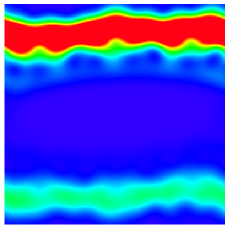
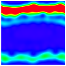
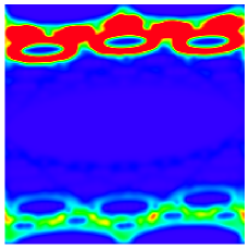
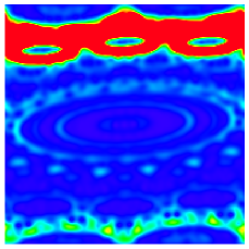
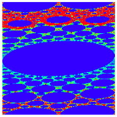
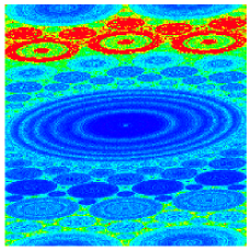
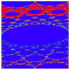
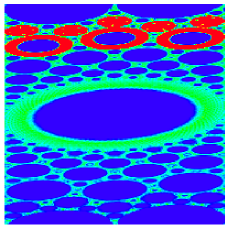
FIG. 1.: Husimi function for the sawtooth map in action angle variables $(p,\theta)$, with $-\pi\leq p<\pi$ (vertical axis) and $0\leq\theta<2\pi$ (horizontal axis), for $K=-0.1$, $T=2\pi/2^{n_{q}}$, $n_{0}=p_{0}/T=[0.38\times 2^{n_{q}}]$, averaged in the interval $950\leq t\leq 1000$. From top to bottom: $n_{q}=6,9,16$ and classical density plot, obtained from an ensemble of $10^{8}$ trajectories, with initial momentum $p_{0}=0.38\times 2\pi$ and random angles. Left and right columns show the case without and with imperfections: in the quantum case the imperfection strength $\epsilon=\delta\tau_{g}$ scales $\propto n_{q}^{-3}$, where $\epsilon=2\times 10^{-3}$ ($n_{q}=6$), $\epsilon=6\times 10^{-4}$ ($n_{q}=9$), $\epsilon=10^{-4}$ ($n_{q}=16$), at $J=0$; in the classical case round-off errors are of amplitude $10^{-3}$. We choose the ratio of the action-angle uncertainties $s=\Delta p/\Delta\theta=1$ ($\Delta p\Delta\theta=T/2$). The color is proportional to the density: blue for zero and red for maximal density.

with $t$ according to the law $f(t)\approx\exp(-At^{2})$. This can be understood as follows: the fluctuations in the individual qubit energies, coupled to the gate operations in time, give effective Rabi oscillations. For this reason $f(t)\sim|\prod_{i=1}^{n_{q}}\cos(\delta_{i}\tau_{g}n_{g}t)|^{2}$ and at short times $f(t)\sim\exp(-n_{q}(\epsilon n_{g}t)^{2})$. This applies also for the case with quantum chaos in the Hamiltonian (3) (e.g. $J=\delta$), which at short time scale can be considered from the viewpoint of Rabi oscillations. Indeed, here we consider small $\epsilon$ and $n_{q}$ values, for which quantum chaos develops on a chaotic time scale $\tau_{\chi}\approx 1/J\sqrt{n_{q}}>>\tau_{g}$ [18]. For example, for $n_{q}=9$, $\epsilon=10^{-4}$, and $J=\delta$ one has $\tau_{\chi}\approx 3\times 10^{3}\tau_{g}$, while one map iteration takes time $\tau_{1}=n_{g}\tau_{g}=413\tau_{g}\approx\tau_{\chi}/10$. The fidelity time scale $t_{f}$ can be obtained from the condition $f(t_{f})=c$, for example $c=0.9$. The above argument gives $t_{f}\propto\epsilon^{-1}n_{g}^{-1}n_{q}^{-1/2}\propto\epsilon^{-1}n_{q}^{-3}$. This estimate is in a good agreement with the numerical data shown in Fig.3. These data also show that $t_{f}$ is not strongly affected by the fact that the internal quantum computer hardware (3) is in the integrable ($J=0$) or quantum chaos ($J=\delta$) regime. The most important point is that the dependence of the fidelity time $t_{f}$ on $n_{q}$ is only polynomial.

FIG. 2.: Fidelity as a function of $t$, for $n_{q}=9$ qubits, $J=\delta$ (solid lines) and $J=0$ (dashed lines). From top to bottom: $\epsilon=10^{-5},3\times 10^{-5},10^{-4},3\times 10^{-4},10^{-3}$.

It is interesting to compare the effect of static imperfections generated by the Hamiltonian (3) in the regime of perfect gates with the case when the static imperfections are absent but the computer operates with noisy gates. To model the noisy gates we put $J=0$ and $\delta_{i}$ fluctuating randomly and independently from one gate to another in the interval $[-\delta/2,\delta/2]$. In this case the fidelity drops in a qualitatively different way $f(t)\approx\exp(-Bt)$ (data not shown). This corresponds to the Fermi golden rule regime, where the probability at a given state decays exponentially with time. At each gate operation a probability of order $\epsilon^{2}$ is transferred to other states, so that the fidelity time scale is given by $t_{f}\sim 1/(\epsilon^{2}n_{g})$. This estimate is in good agreement with numerical data shown in Fig.3. We found the same behavior for $J=\delta=0$ and noisy gates with unitary rotations on a random angle $\epsilon$. The dependence on $\epsilon$ is qualitatively different comparing to the static imperfection case (3) discussed above. We stress that static imperfections give shorter times $t_{f}$ and therefore are more dangerous for quantum computation. We note that the quadratic and linear regimes of fidelity decrease with time were respectively discussed in Refs. [19, 20].

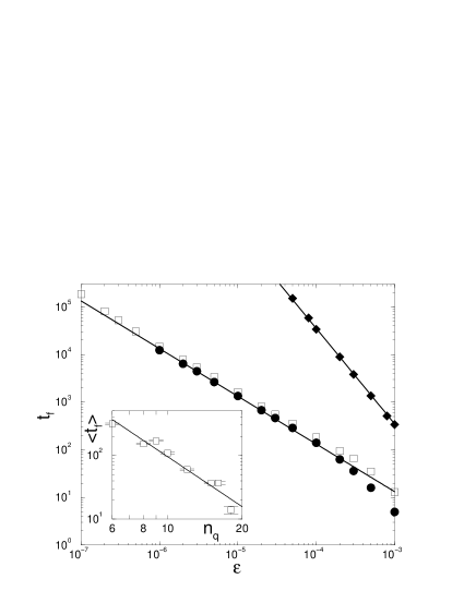
FIG. 3.: Fidelity time scale $t_{f}$ as a function of $\epsilon$, for $n_{q}=9$, in the case of static imperfections ($J=\delta$ (circles) and $J=0$ (squares)) and noisy gates (diamonds, see text). The straight lines have slopes $-1$ and $-2$. The inset shows the dependence of $t_{f}$ on the number of qubits, for $\epsilon=10^{-4}$, $J=0$; the power-law fit (straight line) gives $t_{f}\propto n_{q}^{-2.6}$. Error bars give the statistical errors obtained from $10\leq k\leq 500$ random configurations of static imperfections.

In summary, we have shown that a realistic quantum computer can simulate with exponential efficiency complex dynamics with rich phase space structures. Our studies demonstrate that the main structures inside the localization domain are rather stable in the presence of static imperfections. We show that the errors from static imperfections are stronger than the errors of noisy gates. Of course it is not possible to extract all exponentially large information hidden in the wave function with $2^{n_{q}}$ states. However, it is possible to have access to coarse grained information. For example from a polynomial number of measurements one can obtain the probability distribution over momentum (or angle) states. This allows one to study the anomalous diffusion in the deep semiclassical regime. Such an information is not accessible for classical computers which cannot simulate more than $2^{40}$ quantum states. Recently an efficient algorithm was proposed in Ref. [21], which allows one to measure the value of the Wigner function at a chosen phase space point. This can also provide important new informations about quantum states in systems with hierarchical phase space structures. We believe that in the near future our results can be experimentally observed in quantum computers operating with a small number of qubits.

This work was supported in part by the EC RTN network contract HPRN-CT-2000-0156 and (for D.L.S.) by the NSA and ARDA under ARO contract No. DAAD19-01-1-0553. Support from the PA INFM “Quantum transport and classical chaos” is gratefully acknowledged.

REFERENCES

- [1] For a review see, e.g., A.Steane, Rep. Prog. Phys. 61, 117 (1998).
- [2] P.W. Shor, in Proceedings of the 35th Annual Symposium on Foundations of Computer Science, edited by S. Goldwasser (IEEE Computer Society, Los Alamitos, CA, 1994), p. 124.
- [3] L.K. Grover, Phys. Rev. Lett. 79, 325 (1997).
- [4] S.Lloyd, Science 273, 1073 (1996).
- [5] A. Sørensen and K. Mølmer, Phys. Rev. Lett. 83, 2274 (1999).
- [6] R. Schack, Phys. Rev. A 57, 1634 (1998).
- [7] B. Georgeot and D.L. Shepelyansky, Phys. Rev. Lett. 86, 2890 (2001).
- [8] F. Borgonovi, G.Casati, and B. Li, Phys. Rev. Lett. 77, 4744 (1996); F. Borgonovi, Phys. Rev. Lett. 80, 4653 (1998).
- [9] G. Casati and T. Prosen, Phys. Rev. E 59, R2516 (1999).
- [10] R.E. Prange, R. Narevich, and O. Zaitsev, Phys. Rev. E 59, 1694 (1999).
- [11] See, e.g., A. Ekert and R. Jozsa, Rev. Mod. Phys. 68, 733 (1996).
- [12] C. Monroe, D.M. Meekhof, B.E. King, W.M. Itano, and D.J. Wineland, Phys. Rev. Lett. 75, 4714 (1995).
- [13] L.M.K. Vandersypen, M. Steffen, M.H. Sherwood, C.S. Yannoni, G. Breyta, and I.L. Chuang, Appl. Phys. Lett. 76, 646 (2000).
- [14] Y.S. Weinstein, M.A. Pravia, E.M. Fortunato, S. Lloyd, and D.G. Cory, Phys. Rev. Lett. 86, 1889 (2001).
- [15] I. Dana, N.W. Murray, and I.C. Percival, Phys. Rev. Lett. 62, 233 (1989); Q. Chen, I. Dana, J.D. Meiss, N.W. Murray, and I.C. Percival, Physica D 46, 217 (1990).
- [16] T. Geisel, G. Radons, and J. Rubner, Phys. Rev. Lett. 57, 2883 (1986).
- [17] R.S. MacKay and J.D. Meiss, Phys. Rev. A 37, 4702 (1988).
- [18] B. Georgeot and D.L. Shepelyansky, Phys. Rev. E 62, 3504 (2000); 62, 6366 (2000); G. Benenti, G. Casati, and D.L. Shepelyansky, quant-ph/0009084.
- [19] W.H. Zurek, Phys. Rev. Lett. 53, 391 (1984); V.V. Flambaum, Aust. J. Phys. 53, 489 (2000).
- [20] C. Miquel, J.P. Paz, and W.H. Zurek, Phys. Rev. Lett. 78, 3971 (1997).
- [21] P. Bianucci, C. Miquel, J.P. Paz, and M. Saraceno, quant-ph/0106091; M. Saraceno, private communication.