Optimal simulation of two-qubit Hamiltonians
using general local operations

Abstract

We consider the simulation of the dynamics of one nonlocal Hamiltonian by another, allowing arbitrary local resources but no entanglement nor classical communication. We characterize notions of simulation, and proceed to focus on deterministic simulation involving one copy of the system. More specifically, two otherwise isolated systems $A$ and $B$ interact by a nonlocal Hamiltonian $H\neq H_{A}+H_{B}$. We consider the achievable space of Hamiltonians $H^{\prime}$ such that the evolution $e^{-iH^{\prime}t}$ can be simulated by the interaction $H$ interspersed with local operations. For any dimensions of $A$ and $B$, and any nonlocal Hamiltonians $H$ and $H^{\prime}$, there exists a scale factor $s$ such that for all times $t$ the evolution $e^{-iH^{\prime}st}$ can be simulated by $H$ acting for time $t$ interspersed with local operations. For 2-qubit Hamiltonians $H$ and $H^{\prime}$, we calculate the optimal $s$ and give protocols achieving it. The optimal protocols do not require local ancillas, and can be understood geometrically in terms of a polyhedron defined by a partial order on the set of 2-qubit Hamiltonians.

I Introduction

A Motivation

Like the mythical lovers Thisbe and Pyramus, Alice and Bob wish to be forever in each other’s company, a situation described physically by some many-atom interaction Hamiltonian $H^{\prime}$. Unfortunately their parents disapprove, and have built a massive wall to keep the youngsters apart. Fortunately there is a small hole in the wall, just big enough for one atom of Alice to interact with one atom of Bob via the two-atom interaction Hamiltonian $H$ (Fig. 1). Can they use this limited interaction, together with local operations on each side of the wall, to simulate the desired interaction $H^{\prime}$? Yes, if they are patient, because any nontrivial bipartite interaction can be used both to generate entanglement and to perform classical communication. Therefore they can use $H$, along with local ancillary degrees of freedom on each side of the wall, to generate enough entanglement, and perform enough classical communication to teleport Alice’s entire original state to Bob’s side. Now that they are (virtually) together, Alice and Bob can interact to their heart’s content. When it is time for Alice to go home, they teleport her back to her side, in whatever entangled state they have gotten themselves into, again using $H$ to generate the needed entanglement and perform the needed classical communication. So, by the time they get to be old lovers, Alice and Bob can experience exactly what it would have been like to be young lovers, if they are still foolish enough to want that.

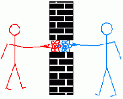
FIG. 1.: Thisbe (L) and Pyramus, separated by a wall, through which they can only interact by a $2$-atom Hamiltonian $H$.

A more practical motivation for studying the ability of nonlocal Hamiltonians to simulate one another comes from quantum control theory [1], in particular the problem of using an experimentally available interaction, together with local operations, to simulate the evolution that would have occurred under some other Hamiltonian not directly accessible to experiment. A more mathematical motivation comes from the desire to parameterize the nonlocal properties of interaction Hamiltonians, so as to characterize the efficiency with which they can be used to simulate one another, and perform other tasks like generating entanglement [2, 3] or performing quantum computation [4, 5, 6, 7]. This parallels the many recent efforts to parameterize the nonlocal properties of quantum states, so as to understand when, and with what efficiency, one quantum state can be converted to another by local operations, or local operations and classical communication. It is not difficult to see, by the Pyramus and Thisbe argument, that all nonlocal Hamiltonians are qualitatively equivalent, in the sense that for any positive $t^{\prime}$ and $\epsilon$, there is a time $t$ such that $t^{\prime}$ seconds of evolution under $H^{\prime}$ can be simulated, with fidelity at least $1\!\!-\!\epsilon$, by $t$ seconds of evolution under $H$, interspersed with local operations; but much work remains to be done on the quantitative efficiency of such simulations.

In this paper we derive bounds on the time efficiency with which one Hamiltonian can simulate another using local resources. In the case of two interacting qubits, we show that these bounds are optimal. The structure of the paper is as follows. In Sec. II, we define the allowed resources and the type of simulation we consider. In Sec. III, we prove some general results on the type of simulation we consider along with some examples. In Sec. IV, we define our goal and summarize our main results for two-qubit Hamiltonians, that are proved in Secs. V and VI. Some discussions and conclusions, and more auxiliary results can be found in Sec. VII, VIII and Apps. A-D. We first describe in more detail some related results.

B Related work

The qualitative equivalence of nonlocal Hamiltonians noted above, and the use of interaction as an infinitesimal generator of entanglement, was already noted several years ago [8]. These discussions also considered the question of interconverting discrete nonlocal primitives, such as nonlocal gates, shared EPR pairs, and uses of a classical bit channel. More generally and quantitatively one may ask, given a nonlocal Hamiltonian $H_{AB}\neq H_{A}+H_{B}$, what is the optimal efficiency with which it can be used, in conjunction with local operations,

• to generate entanglement between $A$ and $B$

• to transmit classical or quantum information from $A$ to $B$, or vice versa

• to simulate the operation of another nonlocal Hamiltonian $H^{\prime}$.

A partial answer to the first question, for two-qubit Hamiltonians, was given by Ref. [2]. The current work is a continuation of previous efforts to study the efficiency simulating one Hamiltonian by another.

Hamiltonian simulation has been considered in the context of quantum computation [4, 5, 6, 7] [9, 10, 11]. In these works the system consists of $n$ qubits, with some given pairwise interaction Hamiltonian. In Refs. [4, 5, 6], the given Hamiltonian was a sum of $\sigma_{z}\otimes\sigma_{z}$ interaction terms between distinct qubits (see Sec. III C for definitions) and the goal was to simulate a particular one of these terms. This was extended in Refs. [7, 10, 11] to arbitrary pairwise interactions, in both the simulating and the simulated Hamiltonians. In these papers the main concern was to obtain methods for simulation, and therefore upper bounds on the resources as a function of $n$.

Independent results on optimizing the time used of a given Hamiltonian for performing certain tasks are reported in Refs. [9, 12, 13]. Reference [9] gives a necessary condition for simulating one $n$-qubit pairwise interaction Hamiltonian by another, and gives a necessary and sufficient condition for simulation with a particular given Hamiltonian. Time resources for simulating the inverse of a Hamiltonian are discussed in Refs. [9, 10, 12]. Reference [13] considers simulating a unitary gate using a given Hamiltonian and a set of controllable gates in the shortest time. A general framework is set up in terms of Riemannian geometry. A time optimal protocol is obtained for the specific Hamiltonian $\sigma_{z}\otimes\sigma_{z}$ in the $2$-qubit case.

Finally, some more recent results have appeared since the original posting of this preprint, extending it and related work in various ways [14, 15, 16, 17] [18, 19, 20, 21].

II Simulation framework

In this section we describe our framework of Hamiltonian simulation, i.e. the rules under which the simulation is to be performed. We also describe other possible frameworks and their relations to the one we adopt.

A Available resources

Let $H$ and $H^{\prime}$ each be a nonlocal Hamiltonian acting on two isolated systems $A$ and $B$. We consider the problem of simulating $H^{\prime}$ by $H$ using unlimited local resources. These include instantaneous local operations and uncorrelated local ancillas of any finite dimensions. It is also necessary to allow some initial classical correlation – Alice and Bob are assumed to have agreed beforehand on their time and spatial coordinates and the simulation protocol to be followed. Besides this, no other nonlocal resources are allowed, neither prior entanglement nor any form of communication beyond what can be achieved through the interaction $H$ itself. Our goal is to minimize the time required of the given Hamiltonian $H$ to simulate another Hamiltonian $H^{\prime}$. This will be defined more formally in Sec. IV.

Note that either the simulating or the simulated system or both can be given the freedom of bringing in local degrees of freedom (ancillas) and allowing interaction between each ancilla with the corresponding local system. Ancillas on the simulated system can make the simulated more powerful and therefore harder to simulate. Ancillas on the simulating system potentially make the simulation easier. We will allow ancillas on the simulating system, though they may not always help (Section VI).

B One-shot and deterministic simulations

In this paper we only concern ourselves with protocols that are one-shot—i.e. operate on a single copy each of the simulated and simulating systems—and that are required to succeed with probability $1$.

More generally, a simulation can be “blockwise”, in which $H^{\otimes n}$ is used for the simulation of $H^{\prime\otimes n}$, or in which $H$ is time-shared among many copies of the system and the amortized cost is considered. A simulation can also be stochastic and fail with finite probability, in which case the expected cost is considered.

C Gate versus dynamics simulations

One possible notion of simulation is that, given $H^{\prime}$ and $t^{\prime}$, we simulate the final unitary evolution $e^{-iH^{\prime}t^{\prime}}$ by composing local operations with elements in the one-parameter family $\{e^{-iHt}\}_{t}$. The final evolution needs to be correct, but the intermediate evolution need not correspond to $e^{-iH^{\prime}t^{\prime\prime}}$ for $0\leq t^{\prime\prime}<t^{\prime}$. The efficiency, given by the ratio $t/t^{\prime}$ can depend on $t^{\prime}$. For example, $H$ can be used to generate entanglement and classical communication to bring $A$ and $B$ together by teleportation, apply $e^{-iH^{\prime}t^{\prime}}$, and teleport $A$ back. Viewing the cost $t$ as a function of $t^{\prime}$, $t$ does not increases indefinitely with $t^{\prime}$, rather, it can be made constant after it reaches a sufficiently large value. As another example, if the nonlocal Hamiltonian $H^{\prime}=\sigma_{z}\otimes\sigma_{z}$ acts for time $t^{\prime}=\pi/2$, the result is the unitary gate $i\sigma_{z}\otimes\sigma_{z}$, which is local, and requires no nonlocal interaction time at all to simulate. This type of simulation, with very different primitives, is much studied in the context of universality of quantum gates (composing a small set of available gates to obtain any desired unitary gate). More recently, simulation of a unitary gate using a fixed given Hamiltonian for a minimal amount of time and local manipulations was studied in Ref. [13] and some partial results were obtained. From now on, we call this type of simulation “gate simulation” or “finite time simulation”.

A natural direction to strengthen the above notion of Hamiltonian simulation is to require not only the end result, but also the intervening dynamics of $H^{\prime}$ to be simulated. Intuitively, one might expect this to mean that the application of $H$, interspersed with instantaneous local operations, produces a trajectory that remains continuously close to the trajectory $e^{-iH^{\prime}t}$ which one wishes to simulate. However, this is impossible in general, because the needed local operations cause the simulating trajectory to be discontinuous, agreeing only intermittently with the trajectory one wishes to simulate. Accordingly we adopt the following definition of dynamics simulation:  The Hamiltonian $H$ simulates the dynamics of $H^{\prime}$ with efficiency $\mu$ if $\forall_{t^{\prime}>0}$, $\forall_{\epsilon>0}$ the unitary operation $e^{-iH^{\prime}t^{\prime}}$ can be simulated with fidelity $\geq 1\!-\!\epsilon$ by some protocol using $H$ for a total time $t^{\prime}/\mu$ and local operations. While this characterization may appear to have given up the idea of approximating the simulated system at intermediate times, in fact it has not, because it can be shown to imply the existence of a $\mu$-efficient “stroboscopic” simulation, which approximates the simulated trajectory arbitrarily closely not only at the begining and end, but also at an arbitrary large set of intermediate times. We discuss this and other simulation notions in Appendix A. We also show that the existence of a protocol for dynamics simulation is equivalent to the existence of one for simulating an infinitesimal time (see Sec. III A) which in turns implies the ability to create protocols for arbitrary finite times by appropriately rescaling and repeating the infinitesimal-time protocol. (see Appendix. D).

III General results and examples

Having defined the simulation framework, we derive some important general results and provide some examples of dynamics simulation, which motivate our main results and simplify some of the later discussions.

A Infinitesimal and time independent simulation

First of all we show that dynamics simulation is equivalent to “infinitesimal simulation”, the problem of simulating the evolution of $H^{\prime}$ for an infinitesimal amount of time $t^{\prime}$. On one hand, any protocol for dynamics simulation simulates the initial evolution, therefore is a protocol for infinitesimal simulation. On the other hand, iterating an infinitesimal simulation results in dynamics simulation. We restrict our attention to infinitesimal simulation from now on, and focus on the lowest order effects in $t^{\prime}$. Note that this property may not hold for other types of simulation described in Appendix A.

Infinitesimal simulation has a very special structure – the optimal simulation protocol is independent of the infinitesimal value of $t^{\prime}$. The proof is included in Appendix D.

B Local Hamiltonians are irrelevant

A general bipartite Hamiltonian $K$ can be written as,

$$K=K_{A}\otimes I+I\otimes K_{B}+\sum_{ij}M_{ij}\,\eta_{i}\otimes\eta_{j}\,,$$ (1)

where $I$ denotes the identity throughout the paper, $K_{A}$, $K_{B}$ are local Hamiltonians acting on $A$, $B$ respectively, and $\{\eta_{i}\}$ is a basis for traceless hermitian operators acting on each of $A$ and $B$. We can “dispose” of the local Hamiltonians $K_{A}$ and $K_{B}$ by undoing them with local unitaries on $A$ and $B$:

$$(e^{iK_{A}t}\otimes e^{iK_{B}t})\;e^{-itK}=e^{-i\,(K-K_{A}\otimes I-I\otimes K_{B})\,t}+{\cal O}(t^{2})\,.$$ (2)

In other words, $K$ can be made to simulate its own nonlocal component.

Likewise, any Hamiltonian can simulate itself with additional local terms. Therefore, given unlimited local resources, the problem of simulating an arbitrary Hamiltonian $H^{\prime}$ by another arbitrary one $H$ reduces to the case when both are purely nonlocal.

C Possible inefficiencies in simulation

Consider the simplest case of two-qubit systems. We introduce the Pauli matrices

$$\sigma_{x}=\left(\begin{array}[]{rr}{0}&{1}\\ {1}&{0}\end{array}\right)\,,~{}~{}\sigma_{y}=\left(\begin{array}[]{rr}{0}&{-i}\\ {i}&{0}\end{array}\right)\,,~{}~{}\sigma_{z}=\left(\begin{array}[]{rr}{1}&{0}\\ {0}&{-1}\end{array}\right)\,,~{}~{}$$ (3)

and the useful identity

$$Ue^{M}U^{\dagger}=e^{UMU^{\dagger}}$$ (4)

where $M$ is any bounded square matrix and $U$ is any unitary matrix of the same dimension.

As an example, let $H=\sigma_{x}\otimes\sigma_{x}$ and $H^{\prime}={1\over 3}(\sigma_{x}\otimes\sigma_{x}+\sigma_{y}\otimes\sigma_{y}+\sigma_{z}\otimes\sigma_{z})$. To simulate $H^{\prime}$ by $H$, let $U_{1}={1\over\sqrt{2}}(\sigma_{x}+\sigma_{y})$ and $U_{2}={1\over\sqrt{2}}(\sigma_{x}+\sigma_{z})$, so that $\sigma_{y}=U_{1}\sigma_{x}U_{1}^{\dagger}$ and $\sigma_{z}=U_{2}\sigma_{x}U_{2}^{\dagger}$. Using Eq. (4), it is easily verified that

$$e^{-iH^{\prime}t^{\prime}}=\left(\rule{0.0pt}{9.04166pt}\right.e^{-iHt^{\prime}/3}\left.\rule{0.0pt}{9.04166pt}\right)\;\times\;\left(\rule{0.0pt}{9.04166pt}\right.U_{1}\otimes U_{1}\;e^{-iHt^{\prime}/3}\;U_{1}^{\dagger}\otimes U_{1}^{\dagger}\left.\rule{0.0pt}{9.04166pt}\right)\;\times\;\left(\rule{0.0pt}{9.04166pt}\right.U_{2}\otimes U_{2}\;e^{-iHt^{\prime}/3}\;U_{2}^{\dagger}\otimes U_{2}^{\dagger}\left.\rule{0.0pt}{9.04166pt}\right)\,.$$ (5)

Conversely, we can simulate $H$ with $H^{\prime}$:

$$e^{-iHt}=e^{-iH^{\prime}3t/2}\;\times\;\left(\rule{0.0pt}{9.04166pt}\right.\sigma_{z}\otimes I\,\;e^{-iH^{\prime}3t/2}\,\;\sigma_{z}\otimes I\left.\rule{0.0pt}{9.04166pt}\right)$$ (6)

Note that the simulating of $H^{\prime}$ for a duration of $t^{\prime}$ requires applying $H$ for a duration of $t^{\prime}$ whereas simulating $H$ for a duration $t$ requires applying $H^{\prime}$ for a duration of $3t$. As the time required of the given Hamiltonian is a resource to be minimized, we see that some simulations are less efficient than the others. In this paper, we are concerned with the inefficiencies of simulation intrinsic to the Hamiltonians $H$ and $H^{\prime}$ that are not caused by a bad protocol. For example, we will show later that the inefficiency in the above example is intrinsic.

D Simulating the zero Hamiltonian – stopping the evolution

In some applications, the given Hamiltonian $H$ cannot be switched on and off. Simulating the zero Hamiltonian ${\bf 0}$ can be viewed as a means for switching off the Hamiltonian $H$ [4, 5, 6]. This can always be done for any dimensions of $A$ and $B$.

First, let $A$ and $B$ be $2^{n}$-dimensional, and

$$H=\sum_{\bf ij}c_{\bf ij}P_{\bf i}\otimes P_{\bf j}\,,$$ (7)

where ${\bf i}$ is a binary vector $(i_{1},i_{2},\cdots,i_{2n})$ that labels the $n$-qubit Pauli matrix $P_{\bf i}=\sigma_{x}^{i_{1}}\sigma_{z}^{i_{2}}\otimes\cdots\otimes\sigma_{x}^{i_{2n\!-\!1}}\sigma_{z}^{i_{2n}}$. It is easily verified that

$${1\over 2^{2n}}\sum_{\bf i}P_{\bf i}MP_{\bf i}={\rm tr}M\;{I\over 2^{n}}\,.$$ (8)

A protocol for simulating ${\bf 0}$ by $H$ is given by,

$$\Pi_{\bf ij}\,(P_{\bf i}\otimes P_{\bf j})\,e^{-iHt/2^{4n}}\,(P_{\bf i}^{\dagger}\otimes P_{\bf j}^{\dagger})~{}=~{}e^{-{it\over 2^{4n}}\sum_{\bf ij}\,(P_{\bf i}\otimes P_{\bf j})\,H\,(P_{\bf i}^{\dagger}\otimes P_{\bf j}^{\dagger})+{\cal O}(t^{2})}~{}\approx~{}e^{-i\,t\,{\rm tr}H/2^{2n}}\,,$$ (9)

in which the net evolution is just an overall phase to the lowest order in $t$.

When $A$ and $B$ are $d$-dimensional, one can embed each of $A$ and $B$ in a larger, $2^{n}$-dimensional system for $n=\lceil\log_{2}d\rceil$ to perform the simulation. Physically, this can be done on each of $A$ and $B$, by attaching a qubit ancilla, extending the Hilbert space to $2d$-dimensions, and applying the simulation to a $2^{n}$-dimensional subspace, such as one spanned by $|i\rangle\otimes|0\rangle$ for $i=1,\cdots,d$ and $|i\rangle\otimes|1\rangle$ for $i=1\cdots 2^{n}\!-d$. Such simulation can also be done without ancillary degrees of freedom, and an alternative method based on Ref. [23] is given in Appendix B.

E Arbitrary but inefficient simulations

We now show that any nonlocal bipartite Hamiltonian can be used to simulate any other, albeit with inefficiencies. In other words, for any $H$ and $H^{\prime}$, operating $H$ for time $t$ can simulate the evolution of $H^{\prime}$ for time $t^{\prime}$ with $t^{\prime}/t>0$. This holds for any dimensions. We keep all definitions from the previous example in the following protocol.

First, let $A$ and $B$ be $2^{n}$-dimensional, $H=\sum_{\bf ij}c_{\bf ij}P_{\bf i}\otimes P_{\bf j}$ and $H^{\prime}=\sum_{\bf ij}c_{\bf ij}^{\prime}P_{\bf i}\otimes P_{\bf j}$. Without loss of generality the coefficient for $P_{\bf k}\otimes P_{\bf k}$ is positive, i.e. $c_{\bf kk}>0$, where ${\bf k}=(0,1,0,\cdots,0)$ and $P_{\bf k}=\sigma_{z}\otimes I\otimes\cdots\otimes I$. It is known that for any $P_{\bf i}$ and $P_{\bf j}$, there exist unitary operations $U_{{\bf ij}\pm}$ in the Clifford group [24], such that

$$U_{{\bf ij}\pm}P_{\bf i}U_{{\bf ij}\pm}^{\dagger}=\pm P_{\bf j}$$ (10)

In other words, one can always transform any $P_{\bf i}$ to any other or to its negation. In our protocol, $H$ simulates $H^{\prime}$ in two steps. First, $H$ simulates $P_{\bf k}\otimes P_{\bf k}$ by:

$$\Pi_{{\bf i,i^{\prime}}|i_{1},i^{\prime}_{1}=0}\;P_{\bf i}\otimes P_{\bf i^{\prime}}\;e^{-iHt/2^{4n\!-\!2}}P_{\bf i}\otimes P_{\bf i^{\prime}}~{}\approx~{}e^{-{it\over 2^{4n\!-\!2}}\sum_{{\bf i,i^{\prime}}|i_{1},i^{\prime}_{1}=0}\!P_{\bf i}\otimes P_{\bf i^{\prime}}HP_{\bf i}\otimes P_{\bf i^{\prime}}}~{}=~{}e^{-i\,t\,c_{\bf kk}P_{\bf k}\otimes P_{\bf k}\,+\,{\rm local~{}terms}}$$ (11)

Alice and Bob independently apply an averaging over all Pauli operators commuting with $P_{\bf k}$, removing all operators except for $I=P_{\bf 0}$ and $P_{\bf k}$ in each of their systems. The local terms can be ignored, following Sec. III B. Second, $P_{\bf k}\otimes P_{\bf k}$ simulates $H^{\prime}$ by:

$$\Pi_{\bf ij}\left(\rule{0.0pt}{9.04166pt}\right.U_{{\bf ki}\;{\rm sg}(\!c_{i\!j}^{\prime}\!)}\otimes U_{{\bf kj}+}\left.\rule{0.0pt}{9.04166pt}\right)\;e^{-iP_{\bf k}\otimes P_{\bf k}|c_{ij}^{\prime}|\>t^{\prime}}\;\left(\rule{0.0pt}{9.04166pt}\right.U_{{\bf ki}\;{\rm sg}(\!c_{i\!j}^{\prime}\!)}\otimes U_{{\bf kj}+}\left.\rule{0.0pt}{9.04166pt}\right)^{\dagger}~{}\approx~{}e^{-it^{\prime}\sum_{\bf ij}P_{\bf i}\otimes P_{\bf j}c_{ij}^{\prime}}~{}=~{}e^{-iH^{\prime}t^{\prime}}$$ (12)

where ${\rm sg}(x)=x/|x|$ if $x\neq 0$ and we omit terms with $c_{ij}^{\prime}=0$ .

When $A$ and $B$ are $d$-dimensional, the simulation of $sH^{\prime}$ by $H$ can again be performed in a larger $2^{n}\times 2^{n}$ system. This method implies a lower bound on the maximum possible value of $s$, $s\geq{1\over 2^{2\lceil\log_{2}d\rceil}}{\max_{\bf ij}|c_{\bf ij}|\over\sum_{\bf ij}|c_{\bf ij}^{\prime}|}$. It is also possible to perform the simulation without ancillas. The proof is given in Appendix C. Other methods for such simulation were independently reported in [18, 19, 20].

F Equivalent classes of local manipulations

Under our simulation framework, Alice and Bob are given unlimited local resources. In this subsection, we show that they only need a relatively small class of manipulations. To facilitate the discussion, we introduce classes of operations $C$, that can be LU, LO, LU$+$anc, and LO$+$anc, to be defined as follows. LU is the class of all local unitaries that act on $A\otimes B$. LU$+$anc is similar, but acts on $(A\otimes A^{\prime})\otimes(B\otimes B^{\prime})$ where $A^{\prime}$ and $B^{\prime}$ are uncorrelated ancillary systems of any finite dimension. LO and LO$+$anc are similarly defined, with the unitaries replaced by general trace-preserving quantum operations. Note that the largest class LO$+$anc corresponds to what is most generally allowed under our simulation framework.

We now show that LU$+$anc, LO, and LO$+$anc are equivalent under our framework. First, we show that LU$+$anc is at least as powerful as LO$+$anc. Any trace preserving quantum operation can be implemented by performing a unitary operation on a larger Hilbert space, followed by discarding the extra degrees of freedom (see, for example, Ref. [25]). The exact difference between LO$+$anc and LU$+$anc is that measurements and tracing are disallowed in the latter. However, these are not needed when simulating Hamiltonian in LU$+$anc, due to the following facts. (1) Measurements can be delayed until the end of the protocol, as operations conditioned on intermediate measurement results can be implemented unitarily. (2) In Hamiltonian simulation, the ancillary systems $A^{\prime}B^{\prime}$ have to be disentangled from $AB$ at the end of the simulation. Thus no actual measurement or discard is needed. These facts allow any LO$+$anc protocol to be reexpressed as an LU$+$anc protocol with pure product state ancillas, meaning that LO and LO$+$anc are no more powerful than LU$+$anc. Conversely, due to fact (2) above, any LU$+$anc protocol can be viewed as an LO protocol. Thus, we establish the equivalence between LO, LU$+$anc, and LO$+$anc. From now on, we focus on LU$+$anc protocols for full generality, and on LU protocols as a possible restriction.

IV Formal statement of the problem and summary of results

Let $H$, $H^{\prime}$, $A$, $B$, $A^{\prime}$, $B^{\prime}$ be defined as before.

Definition: $H^{\prime}$ can be efficiently simulated by $H$,

$$H^{\prime}\leq_{C}H,$$ (13)

if the evolution according to $e^{-iH^{\prime}t^{\prime}}$ for any time $t^{\prime}$ can be simulated by using the Hamiltonian $H$ for the same time $t^{\prime}$ and using manipulations in the class $C$.

Definition: $H^{\prime}$ and $H$ are equivalent under the class $C$,

$$H^{\prime}\equiv_{C}H,$$ (14)

if $H^{\prime}\leq_{C}H$ and $H^{\prime}\leq_{C}H$.

Throughout the paper, we only consider LU$+$anc protocols following Sec. III F. We also restrict attention to $H$ and $H^{\prime}$ that are purely nonlocal, following Sec. III B.

An LU$+$anc protocol simulates $H^{\prime}$ with $H$ by interspersing the evolution of $H$ with local unitaries on $AA^{\prime}$ and $BB^{\prime}$. More specifically, the most general protocol for simulating $H^{\prime}$ using $H$ for a total time $t$ is to attach the ancillas $A^{\prime}B^{\prime}$ in the state $\mbox{$|0_{A^{\prime}}\rangle$}\otimes\mbox{$|0_{B^{\prime}}\rangle$}$, apply some $U_{1}\otimes V_{1}$, evolve $AB$ according to $H$ for some time $t_{1}$, apply $U_{2}\otimes V_{2}$, further evolve $AB$ according to $H$ for time $t_{2}$, and iterate “apply $U_{i}\otimes V_{i}$ and evolve with $H$ for time $t_{i}$” some $n$ times. At the end, it applies a final $U_{f}\otimes V_{f}$. The $t_{i}>0$ are constrained by $\sum_{i=1}^{n}t_{i}=t$. Suppose the protocol indeed simulates an evolution for time $t^{\prime}$ according to $H^{\prime}$. Then we can write

$$\left(\rule{0.0pt}{10.33327pt}\right.U_{f}\otimes V_{f}\times U_{n}\otimes V_{n}\;e^{-iHt_{n}}\;U_{n}^{\dagger}\otimes V_{n}^{\dagger}\times\cdots\times U_{1}\otimes V_{1}\;e^{-iHt_{1}}\;U_{1}^{\dagger}\otimes V_{1}^{\dagger}\left.\rule{0.0pt}{10.33327pt}\right)\;|\psi\rangle\otimes|0_{A^{\prime}}\rangle\otimes|0_{B^{\prime}}\rangle\hskip 86.11084pt$$ (15)

$$\hskip 215.2771pt=\left(\rule{0.0pt}{9.04166pt}\right.e^{-iH^{\prime}t^{\prime}}|\psi\rangle\left.\rule{0.0pt}{9.04166pt}\right)\otimes\left(\rule{0.0pt}{9.04166pt}\right.W_{A^{\prime}B^{\prime}}(t_{1},\cdots,t_{n})|0_{A^{\prime}}\rangle\otimes|0_{B^{\prime}}\rangle\left.\rule{0.0pt}{9.04166pt}\right)\,,$$ (16)

where we have redefined $U_{i=1,2,\cdots,n}$ and $V_{i=1,2,\cdots,n}$, and $|\psi\rangle$ denotes the initial state in $AB$. In Eq. (16), $e^{-iHt_{i}}$ acts on $AB$ and implicitly means $e^{-iHt_{i}}\otimes I_{A^{\prime}B^{\prime}}$. The operator $W_{A^{\prime}B^{\prime}}(t_{1},\cdots,t_{n})$ describes the residual transformation of $A^{\prime}B^{\prime}$, and can be chosen to be unitary since the operation on the left hand side of Eq. (16) is unitary. The problem we are concerned with can be stated in two equivalent ways:

Optimal and efficient simulation: Let $H$ be arbitrary. The optimal simulation problem is to, for each $H^{\prime}$, find a solution $\{U_{i}\}$, $\{V_{i}\}$, $\{t_{i}\}$ of Eq. (16) such that $t^{\prime}/t$ is maximal. The efficient simulation problem is to characterize every $H^{\prime}$ which admits a solution for Eq. (16) with $t^{\prime}=t$, i.e. $H^{\prime}\leq_{{\rm LU}+{\rm anc}}H$.

Definition: The optimal simulation factor $s_{H^{\prime}|H}$ under class $C$ of operations is the maximal $s>0$ such that $sH^{\prime}\leq_{C}H$.

The optimal and efficient simulation problems are equivalent because inefficient simulation is always possible (see Section III). The efficient simulation problem can be solved by finding the optimal solution for each $H^{\prime}$ and characterizing those with $t^{\prime}/t\geq 1$. The optimal simulation problem can be solved by finding the maximum $s$ for which $sH^{\prime}$ is efficiently simulated. With this in mind, we may talk of solving either problem throughout the paper.

We now summarize our results. We show in Appendix D that, in the infinitesimal regime, the most general simulation protocol Eq. (16) using LU$+$anc is equivalent to

$$sH^{\prime}=\mbox{$\langle 0_{A^{\prime}}|$}\otimes\mbox{$\langle 0_{B^{\prime}}|$}\sum_{i}\;p_{i}\;U_{i}\otimes V_{i}\;(H\otimes I_{A^{\prime}B^{\prime}})\;U_{i}^{\dagger}\otimes V_{i}^{\dagger}\;\mbox{$|0_{A^{\prime}}\rangle$}\otimes\mbox{$|0_{B^{\prime}}\rangle$}\,.$$ (17)

In the LU case (without ancillas), Eq. (17) reads

$$sH^{\prime}=\sum_{i}\;p_{i}\;U_{i}\otimes V_{i}\;H\;U_{i}^{\dagger}\otimes V_{i}^{\dagger}\,,$$ (18)

where $t=t_{1}+\cdots+t_{n}$, $p_{k}=t_{k}/t$, and $s={t^{\prime}\over t}$. Thus, the set $\{H^{\prime}\leq_{\rm LU}H\}$ is precisely the convex hull of the set $\{U\otimes V\;H\;U^{\dagger}\otimes V^{\dagger}\}$ when $U$ and $V$ range over all unitary matrices on $A$ and $B$ respectively. The linear dependence of ${t^{\prime}\over t}H^{\prime}$ on $H$ is manifest in both Eq. (17) and Eq. (18).

Our main results apply to the simulation of two-qubit Hamiltonians, and are summarized as follows:

Result 1: Any simulation protocol using LU$+$anc can be replaced by one using LU with the same simulation factor. This will be proved in Section VI. Thus, the four partial orders $\leq_{\rm LU}$, $\leq_{{\rm LU}+{\rm anc}}$, $\leq_{\rm LO}$, $\leq_{{\rm LO}+{\rm anc}}$ are equivalent for two-qubit Hamiltonians.

Result 2: We present the necessary and sufficient conditions for $H^{\prime}\leq_{LU}H$, for arbitrary two-qubit Hamiltonians $H$ and $H^{\prime}$, and find the optimal simulation factor $s_{H^{\prime}|H}$ and the optimal simulation strategy in terms of $\{U_{i}\},\{V_{i}\},\{t_{i}\}$. This will be discussed in Section V.

These results naturally endow the set of two-qubit Hamiltonians with a partial order $\leq_{C}$. This induces for each $H$, a set $\{H^{\prime}:H^{\prime}\leq_{C}H\}$ which is convex: if $H^{\prime}\leq_{C}H$ and $H^{\prime\prime}\leq_{C}H$, $pH^{\prime}+(1-p)H^{\prime\prime}\leq_{C}H$ for any $0\leq p\leq 1$. Our method relies on the convexity of the set $\{H^{\prime}:H^{\prime}\leq_{C}H\}$, which has a simple geometric description, and in turns allows the partial order $\leq_{C}$ to be succinctly characterized by a majorization-like relation. The geometric and majorization interpretations offer two different methods to obtain, in practice, the optimal protocol and the simulation factor.

V Optimal LU simulation of two-qubit Hamiltonians

We will prove that $\leq_{\rm LU}$ is equivalent to $\leq_{{\rm LU}+{\rm anc}}$ in the next section. In this section, we focus on LU simulations. We first adapt a result from Ref. [2] to reduce the problem to a smaller set of two-qubit Hamiltonians $H$ and $H^{\prime}$. Then, for any $H$, we identify the set $\{H^{\prime}:H^{\prime}\leq_{C}H\}$ with a simple polyhedron and obtain simple geometric and algebraic characterizations of it. The optimal solution for each pair of $H$ and $H^{\prime}$ is derived. Finally, the problem is rephrased in the language of majorization.

A Normal form for two-qubit Hamiltonians

The most general purely nonlocal two-qubit Hamiltonian $K$ can be written as,

$$K=\sum_{ij}M_{ij}\,\sigma_{i}\otimes\sigma_{j}\,,$$ (19)

where the summation is over Pauli matrices $i,j=x,y,z$ or $1,2,3$ throughout the discussion for two-qubit Hamiltonians. Let

$$H=\sum_{i}h_{i}\,\sigma_{i}\otimes\sigma_{i},$$ (20)

where $h_{1}\geq h_{2}\geq|h_{3}|$ are the singular values of the $3\times 3$ matrix $M$ with entries $M_{ij}$, and $h_{3}={\rm sg}(\det M)|h_{3}|$. We say $H$ is the normal form of $K$.

Theorem: Let $H$ be the normal form of $K$. Then $H\equiv_{\rm LU}K$.

Proof: If the local unitaries $U^{\dagger}\otimes V^{\dagger}$ and $U\otimes V$ are applied before and after $e^{-iKt}$, the resulting evolution is given by

$$e^{-iK^{\prime}t}=U\otimes V\;e^{-iKt}\;U^{\dagger}\otimes V^{\dagger}=e^{-i\;(U\otimes V)\;K(U^{\dagger}\otimes V^{\dagger})\;t}\,,$$ (21)

with

$$K^{\prime} = (U\otimes V)\;K\;(U^{\dagger}\otimes V^{\dagger})$$ (22)

$$= \sum_{ij}M_{ij}\;(U\sigma_{i}U^{\dagger})\otimes(V\sigma_{j}V^{\dagger})$$ (23)

$$= \sum_{ij}M_{ij}\left(\rule{0.0pt}{10.33327pt}\right.\sum_{l}R_{il}\sigma_{l}\left.\rule{0.0pt}{10.33327pt}\right)\otimes\left(\rule{0.0pt}{10.33327pt}\right.\sum_{k}S_{jk}\sigma_{k}\left.\rule{0.0pt}{10.33327pt}\right)$$ (24)

$$= \sum_{lk}\left(\rule{0.0pt}{9.04166pt}\right.R^{T}MS\left.\rule{0.0pt}{9.04166pt}\right)_{lk}\;\sigma_{l}\otimes\sigma_{k}\;\equiv\;\sum_{lk}M^{\prime}_{lk}\;\sigma_{l}\otimes\sigma_{k}$$ (25)

In Eq. (24), $R,S\in$ SO(3) since conjugating $\vec{r}\cdot\vec{\sigma}$ by SU(2) matrices corresponds to rotating $\vec{r}$ by a matrix in SO(3) (and vice versa). Equation (25) implies that $K^{\prime}=U\otimes VKU^{\dagger}\otimes V^{\dagger}$ for some unitary $U,V$ if and only if $M^{\prime}=R^{T}MS$. In particular, there is a choice of $R$ and $S$ that makes $K^{\prime}=H$:

$$R^{T}=\left(\begin{array}[]{ccc}{1}&{0}&{0}\\ {0}&{1}&{0}\\ {0}&{0}&{\det O_{1}}\end{array}\right)\times O_{1}^{T}\,,~{}~{}~{}S=O_{2}^{T}\times\left(\begin{array}[]{ccc}{1}&{0}&{0}\\ {0}&{1}&{0}\\ {0}&{0}&\det O_{2}\end{array}\right)$$ (26)

where $M=O_{1}D\,O_{2}$ is the singular value decomposition of $M$, with $O_{1},O_{2}\in$ O(3) and $D={\rm diag}(h_{1},h_{2},|h_{3}|)$. Thus $K$ and $H$ are related by a conjugation by local unitaries, which implies $K\equiv_{\rm LU}H$.

As suggested by the above proof, we define a few useful notations.

Definitions We call the $3\times 3$ real matrix $M_{ij}$ the “Pauli representation” of $K$, when $M$ and $K$ are related by Eq. (19). We use $D_{K}$ to denote a diagonal Pauli representation of $K$.

Since any 2-qubit Hamiltonian is equivalent to its normal form, we assume $H^{\prime}$, $H$ are in normal forms from now on. We now turn to LU simulation of $H^{\prime}$ by $H$.

B General LU simulation of normal form two-qubit Hamiltonians

Recall from Eq. (18) in Section IV that the most general simulation using LU is given by

$$sH^{\prime}=p_{1}\;U_{1}\otimes V_{1}\;H\;U_{1}^{\dagger}\otimes V_{1}^{\dagger}+\cdots+p_{n}\;U_{n}\otimes V_{n}\;H\;U_{n}^{\dagger}\otimes V_{n}^{\dagger}$$ (27)

where $s=t^{\prime}/t$. Following the discussion in Section V A, we only need to consider $H=\sum_{i}h_{i}\;\sigma_{i}\otimes\sigma_{i}$ and $H^{\prime}=\sum_{i}h_{i}^{\prime}\;\sigma_{i}\otimes\sigma_{i}$ that are in their normal forms. The Pauli representation of $(U\otimes V)H(U^{\dagger}\otimes V^{\dagger})$ is given by $RD_{H}S$ for some $R,S\in$ SO(3). We can reexpress Eq. (27) as

$$sD_{H^{\prime}}=p_{1}\;R_{1}D_{H}S_{1}+\cdots+p_{n}\;R_{n}D_{H}S_{n}$$ (28)

where $R_{i},S_{i}\in SO(3)$. Since $H$ and $H^{\prime}$ are in their normal form, $h_{1}\geq h_{2}\geq|h_{3}|$ and $h_{1}^{\prime}\geq h_{2}^{\prime}\geq|h_{3}^{\prime}|$. Without loss of generality, we can make two assumptions. First, we can assume $h_{3}\geq 0$: If $h_{3}<0$, we can right-multiply Eq. (28) by $S={\rm diag}(1,1,-1)$:

$$sD_{H^{\prime}}S=p_{1}\;R_{1}(D_{H}S)(SS_{1}S)+\cdots+p_{n}\;R_{n}(D_{H}S)(SS_{n}S)$$ (29)

in which $SS_{i}S\in$ SO(3), and $D_{H}S={\rm diag}(h_{1},h_{2},|h_{3}|)$ is of the desired form. Thus, we can assume $h_{3}\geq 0$. Second, note that $s_{H^{\prime}|H}=as_{H^{\prime}|aH}={1\over a}s_{aH^{\prime}|H}$. The protocol is unchanged when Eq. (28) is divided by ${\rm tr}D_{H}=h_{1}+h_{2}+h_{3}$. Therefore, without loss of generality, the normalization $h_{1}+h_{2}+h_{3}=1$ can be assumed.

Equations (27) and (28) have a simple physical interpretation: the protocol partitions the allowed usage of $H$ ($D_{H}$) into different $U_{k}\otimes V_{k}\;H\;U_{k}^{\dagger}\otimes V_{k}^{\dagger}$ ($R_{k}DS_{k}$), resulting in an “average Hamiltonian” $H^{\prime}$ ($D_{H^{\prime}}$), which is a convex combination of the $U_{k}\otimes V_{k}\;H\;U_{k}^{\dagger}\otimes V_{k}^{\dagger}$ ($R_{k}DS_{k}$).

The Hamiltonians, represented by $D_{H^{\prime}}$, that can be efficiently simulated ($s=1$) correspond to the diagonal elements of the convex hull of $\{RD_{H}S:R,S\in{\rm SO(3)}\}$. We call this diagonal subset, which is also convex, ${\cal C}_{H}$. Note that the zero Hamiltonian is in the interior of ${\cal C}_{H}$, because $H$ can simulate any $sH^{\prime}$ for small $s$ without ancillas (see Section III). Thus $\forall~{}D_{H^{\prime}}\neq 0$, the optimal solution is a boundary point of ${\cal C}_{H}$. The problem of efficient or optimal simulation can be rephrased:

Given $H$, let ${\cal C}_{H}$ be the diagonal subset of the convex hull of $\{RD_{H}S:R,S\in{\rm SO(3)}\}$. Then $H^{\prime}$ can be efficiently simulated by $H$ if and only if $D_{H^{\prime}}\in{\cal C}_{H}$. For any $H^{\prime}$, $s_{H^{\prime}|H}D_{H^{\prime}}$, which represents the optimal simulation, is the unique intersection of the semi-line $\lambda D_{H^{\prime}}$ ($\lambda\geq 0$) with the boundary of ${\cal C}_{H}$. The optimal protocol can be obtained by decomposing $s_{H^{\prime}|H}\,D_{H^{\prime}}$ in terms of the extreme points of ${\cal C}_{H}$.

Since each point in ${\cal C}_{H}$ can be decomposed as a convex combination of the extreme points of ${\cal C}_{H}$, each efficiently simulated Hamiltonian can be identified with a simulation protocol and vice versa. We will refer to elements in ${\cal C}_{H}$ as Hamiltonians or simulation protocols interconvertibly.

Central to our problem is the structure of ${\cal C}_{H}$. We will show in Sec. V D that it is a simple polyhedron that we call ${\cal P}_{H}$. Its set of vertices, $P_{24}$, is a subset of ${\cal C}_{H}$ containing $24$ elements. They are obtained from $D_{H}$ by permuting the diagonal elements and putting an even number of $-$ signs. More explicitly, these elements are $\pi_{i}D_{H}\pi_{i}s_{j}$, where

$$\pi_{0}=I\,,~{} \pi_{1}=\left[\begin{array}[]{ccc}-1&0&0\\ 0&0&1\\ 0&1&0\end{array}\right]\,,~{}\pi_{2}=\left[\begin{array}[]{ccc}0&0&1\\ 0&-1&0\\ 1&0&0\end{array}\right]\,,~{}\pi_{3}=\left[\begin{array}[]{ccc}0&1&0\\ 1&0&0\\ 0&0&-1\end{array}\right]\,,~{}\pi_{4}=\left[\begin{array}[]{ccc}0&1&0\\ 0&0&1\\ 1&0&0\end{array}\right]\,,~{}\pi_{5}=\left[\begin{array}[]{ccc}0&0&1\\ 1&0&0\\ 0&1&0\end{array}\right]\,,~{}$$ (45)

$$s_{0}=I\,,~{} s_{1}=\left[\begin{array}[]{ccc}1&0&0\\ 0&-1&0\\ 0&0&-1\end{array}\right]\,,~{}s_{2}=\left[\begin{array}[]{ccc}-1&0&0\\ 0&1&0\\ 0&0&-1\end{array}\right]\,,~{}s_{3}=\left[\begin{array}[]{ccc}-1&0&0\\ 0&-1&0\\ 0&0&1\end{array}\right]\,.$$ (55)

The transformation $D_{H}\rightarrow\pi_{i}D_{H}\pi_{i}^{\dagger}s_{j}$ is physically achieved by $H\rightarrow(U_{\pi_{i}}^{\dagger}\!\otimes U_{s_{j}}U_{\pi_{i}})\,H\,(U_{\pi_{i}}\!\otimes U_{s_{j}}^{\dagger}U_{\pi_{i}}^{\dagger})$, where $U_{\pi_{i}}=(\sigma_{j}+\sigma_{k})/\sqrt{2}$ for $i=1,2,3$ and $i,j,k$ distinct, $U_{\pi_{i}}=\cos(\pi/3)I\pm i\sin(2\pi/3)(\sigma_{x}+\sigma_{y}+\sigma_{z})/\sqrt{3}$ for $i=4,5$, and $U_{s_{i}}=\sigma_{i}$ for $i=1,2,3$. These can be verified using Eq. (24). The fact that $P_{24}$ is the set of extreme points of ${\cal C}_{H}$ means that any optimal simulation protocol only involves the transformations $D_{H}\rightarrow\pi_{i}D_{H}\pi_{i}s_{j}$.

In the next few subsections, we investigate the geometry of ${\cal P}_{H}$, prove that ${\cal C}_{H}={\cal P}_{H}$, and find the optimal solution for any $H^{\prime}$ using the fact ${\cal C}_{H}={\cal P}_{H}$. Then, we restate the solution in terms of a majorization-like relation.

C The Polyhedron ${\cal P}_{H}$

Since $P_{24}$ and ${\cal P}_{H}$ consist of diagonal matrices only, their elements can be represented by real $3$-dimensional vectors. The defining characterization of ${\cal P}_{H}$ is the polyhedron with $24$ (not necessarily distinct) vertices that are elements of $P_{24}$. We now turn to a useful characterization of ${\cal P}_{H}$ as the region enclosed by its faces,

$$(x,y,z)\in{\cal P}_{H}~{}{\rm iff}\left\{\begin{array}[]{l}~{}~{}|x|\leq h_{1}~{},|y|\leq h_{1}~{},|z|\leq h_{1}\\ -(1-2h_{3})\leq+x+y+z\leq 1\\ -(1-2h_{3})\leq-x-y+z\leq 1\\ -(1-2h_{3})\leq+x-y-z\leq 1\\ -(1-2h_{3})\leq-x+y-z\leq 1\end{array}\right.$$ (56)

where the fact that $H$ is in normal form, $h_{3}\geq 0$, and that $h_{1}+h_{2}+h_{3}=1$ are used to replace the bounds $\sum_{i}h_{i}$ and $-(\sum_{i}h_{i}-2\min_{i}h_{i})$ by $1$ and $-(1-2h_{3})$ in Eq. (56). Equation (56) can be used to determine whether a point, as specified by its coordinates, is in ${\cal P}_{H}$ or not. The validity of Eq. (56) can be proved by plotting $P_{24}$ (and therefore ${\cal P}_{H}$) and verifying that the faces are as given in Eq. (56). We first plot ${\cal P}_{H}$ for the simple case $(h_{1},h_{2},h_{3})=(1,0,0)$, for which $P_{24}$ has $6$ distinct points: $(\pm 1,0,0)$, $(0,\pm 1,0)$, $(0,0,\pm 1)$ and Eq. (56) holds trivially:

(57)

Now, we plot ${\cal P}_{H}$ for the most complicated case, $h_{1}>h_{2}>h_{3}>0$ in Fig. (58):

(58)

As in Fig. (57), Fig. (58) is viewed from the direction $(1,1,1)$. Three faces are removed to show the structure in the back. There are $3$ types of faces. There are $6$ identical rectangular purple faces on the planes $x=\pm h_{1},y=\pm h_{1},z=\pm h_{1}$. There are two groups each consists of $4$ identical hexagonal faces. The first group of $4$ consists of the $3$ light blue faces in the back, and the light blue face in the front. These are the truncated faces of the original octahedron, lying on the planes $x+y+z=1,-x+y-z=1,-x-y+z=1,x-y-z=1$. The second group consists of the $3$ empty faces in the front, and the white face in the back. They are inside the original octahedron and are parallel to the original faces. They lie on the planes $-x-y-z=1-2h_{3},-x+y+z=1-2h_{3},x-y+z=1-2h_{3},x+y-z=1-2h_{3}$. Note that each hexagon in one group has a parallel counterpart in the other group. All together, there are $7$ pairs of parallel faces, each pair bounds one expression in Eq. (56). It is straightforward to verify the diagram and Eq. (56).

The plots for other cases, such as when $h_{3}=0$ or $h_{1}=h_{2}$, can be likewise obtained and Eq. (56) be verified. These are generally simpler then Fig. (58), and may admit simpler solutions in Section V E. However, we leave the details to the interested readers and move on to prove that ${\cal C}_{H}={\cal P}_{H}$.

D Proof of ${\cal C}_{H}={\cal P}_{H}$

We now show that ${\cal C}_{H}={\cal P}_{H}$. Recall that ${\cal C}_{H}$ consists of Hamiltonians that can be expressed as $D_{H^{\prime}}=\sum_{i}p_{i}\;R_{i}D_{H}S_{i}^{T}$ (by putting $s=1$ in Eq. (28) and using $S_{i}^{T}$ in place of $S_{i}$). The fact that $D_{H^{\prime}}$ is diagonal implies that only the diagonal elements in each $R_{i}D_{H}S_{i}^{T}$ contribute to $D_{H^{\prime}}$; it is possible for an individual $R_{i}D_{H}S_{i}^{T}$ to be off-diagonal, but the off-diagonal elements have to cancel out in the sum. To show that ${\cal C}_{H}={\cal P}_{H}$, it suffices to show that the diagonal part of each $R_{i}D_{H}S_{i}^{T}$ is in ${\cal P}_{H}$, because any $D_{H^{\prime}}\in{\cal C}_{H}$ will then be in ${\cal P}_{H}$.

Let us consider the diagonal part of $RD_{H}S^{T}$, represented as a $3$-dimensional vector $(g_{1},g_{2},g_{3})$. Since $D_{H}={\rm diag}(h_{1},h_{2},h_{3})$,

$$g_{i}=(RD_{H}S^{T})_{ii}=\sum_{k}R_{ik}h_{k}S^{T}_{ki}=\sum_{k}R_{ik}S_{ik}h_{k}\,.$$ (59)

The vectors $(h_{1},h_{2},h_{3})$ and $(g_{1},g_{2},g_{3})$ are linearly related by

$$\left[\begin{array}[]{c}g_{1}\\ g_{2}\\ g_{3}\end{array}\right]=R\mbox{.{\fds*}\hskip 0.43057pt}S\left[\begin{array}[]{c}h_{1}\\ h_{2}\\ h_{3}\end{array}\right]\,,$$ (60)

where $.*$ denotes the entry-wise multiplication of two matrices, also known as the Schur product or the Hadamard product. It is useful to expand $g_{i}$ in Eq. (59) explicitly

$$g_{i}=R_{i1}\,S_{i1}\;h_{1}+R_{i2}\,S_{i2}\;h_{2}+R_{i3}\,S_{i3}\;h_{3}\,.$$ (61)

Then, we can prove the first group of inequalities

$$|g_{i}|\leq|R_{i1}S_{i1}|\;h_{1}+|R_{i2}S_{i2}|\;h_{2}+|R_{i3}S_{i3}|\;h_{3}\leq\max_{i}h_{i}=h_{1}$$ (62)

We use the fact that $R,S\in$ SO(3) to prove the second inequality: $R,S$ consists of orthonormal rows and columns. Hence, $(|R_{i1}|,|R_{i2}|,|R_{i3}|)$ and $(|S_{i1}|,|S_{i2}|,|S_{i3}|)$ are unit vectors, and their inner product $|R_{i1}S_{i1}|+|R_{i2}S_{i2}|+|R_{i3}S_{i3}|\leq 1$. We refer to this argument, which is frequently used, as the “inner product argument”. The second group of inequalities can be proved by

$$\sum_{i}|g_{i}|=\sum_{i}\left|\rule{0.0pt}{10.33327pt}\right.\sum_{k}R_{ik}S_{ik}\;h_{k}\left.\rule{0.0pt}{10.33327pt}\right|\leq\sum_{k}\left(\rule{0.0pt}{10.33327pt}\right.\sum_{i}|R_{ik}||S_{ik}|\left.\rule{0.0pt}{10.33327pt}\right)|h_{k}|\leq\sum_{k}h_{k}=1\,.$$ (63)

The second inequality in Eq. (63) is due to $\sum_{i}|R_{ik}||S_{ik}|\leq 1$, obtained again by the inner product argument. This proves all of

$$g_{1}+g_{2}+g_{3}\leq 1\,,~{}~{}g_{1}-g_{2}-g_{3}\leq 1\,,~{}~{}-g_{1}+g_{2}-g_{3}\leq 1\,,~{}~{}-g_{1}-g_{2}+g_{3}\leq 1$$ (64)

Finally,

$$g_{1}+g_{2}+g_{3}=\left(\!\!\begin{array}[]{r}R_{11}\,S_{11}\\ +R_{21}\,S_{21}\\ +R_{31}\,S_{31}\end{array}\!\right)h_{1}+\left(\!\!\begin{array}[]{r}R_{12}\,S_{12}\\ +R_{22}\,S_{22}\\ +R_{32}\,S_{32}\end{array}\!\right)h_{2}+\left(\!\!\begin{array}[]{r}R_{13}\,S_{13}\\ +R_{23}\,S_{23}\\ +R_{33}\,S_{33}\end{array}\!\right)h_{3}=\lambda_{1}h_{1}+\lambda_{2}h_{2}+\lambda_{3}h_{3}$$ (65)

where $\lambda_{i}$ is the coefficient of $h_{i}$ in the parenthesis. The inner product argument implies $|\lambda_{i}|\leq 1$. Moreover, we will prove $\sum_{i}\lambda_{i}\geq-1$ shortly, which implies

$$g_{1}+g_{2}+g_{3} \geq \lambda_{1}h_{1}+\lambda_{2}h_{2}+(-1-\lambda_{1}-\lambda_{2})h_{3}$$ (66)

$$= \lambda_{1}(h_{1}-h_{3})+\lambda_{2}(h_{2}-h_{3})-h_{3}$$ (67)

$$\geq -h_{1}-h_{2}+h_{3}=-(1-2h_{3})$$ (68)

where Eq. (68) is the minimum of the previous line, attained at $\lambda_{1}=\lambda_{2}=-1$ and $\lambda_{3}=1$. We now prove $\sum_{i}\lambda_{i}\geq-1$. First,

$$\sum_{i}\lambda_{i}=R_{11}S_{11}+R_{21}S_{21}+R_{31}S_{31}+R_{12}S_{12}+R_{22}S_{22}+R_{32}S_{32}+R_{13}S_{13}+R_{23}S_{23}+R_{33}S_{33}={\rm tr}(R^{T}S)$$ (69)

As $R,S\in$ SO(3), $R^{T}S\in$ SO(3). Each SO(3) matrix is a spatial rotation, therefore having the eigenvalue $+1$ that corresponds to the vector defining the rotation axis. Moreover, any SO(3) matrix has determinant $1$. Therefore, the eigenvalues are generally given by $1$, $e^{i\phi}$, $e^{-i\phi}$ and the trace is $1+2\cos(\phi)\geq-1$. This completes the proof of Eq. (68). The last $3$ of the $4$ inequalities

$$+g_{1}+g_{2}+g_{3}\geq-(1-2h_{3})\,,~{}~{}+g_{1}-g_{2}-g_{3}\geq-(1-2h_{3})\,,$$ (70)

$$-g_{1}+g_{2}-g_{3}\geq-(1-2h_{3})\,,~{}~{}-g_{1}-g_{2}+g_{3}\geq-(1-2h_{3})\,,$$ (71)

can be proved similarly. For example, consider

$$g_{1}-g_{2}-g_{3}=\left(\!\!\begin{array}[]{r}R_{11}\,S_{11}\\ -R_{21}\,S_{21}\\ -R_{31}\,S_{31}\end{array}\!\right)h_{1}+\left(\!\!\begin{array}[]{r}R_{12}\,S_{12}\\ -R_{22}\,S_{22}\\ -R_{32}\,S_{32}\end{array}\!\right)h_{2}+\left(\!\!\begin{array}[]{r}R_{13}\,S_{13}\\ -R_{23}\,S_{23}\\ -R_{33}\,S_{33}\end{array}\!\right)h_{3}\,.$$ (72)

The previous argument for $g_{1}+g_{2}+g_{3}$ applies by redefining $R$ to be $\left[\begin{array}[]{rrr}{1}&{0}&{0}\\ {0}&{-1}&{0}\\ {0}&{0}&{-1}\end{array}\right]\times R$.

Altogether, the inequalities in Eqs. (62), (63), and (71) satisfied by $(g_{1},g_{2},g_{3})$ are precisely the defining inequalities for ${\cal P}_{H}$ in Eq. (56). Therefore, the diagonal part of any $RD_{H}S^{T}$ is in ${\cal P}_{H}$, and ${\cal C}_{H}={\cal P}_{H}$.

E Optimization over ${\cal P}_{H}$

Having proved ${\cal C}_{H}={\cal P}_{H}$, we can solve the optimal simulation problem given $D_{H}$ and $D_{H^{\prime}}$ by finding the unique intersection of the semi-line $\lambda D_{H^{\prime}}$ with the boundary of ${\cal P}_{H}$ (see Section V B). We now explicitly work out $s_{H|H^{\prime}}$, i.e. the value of $\lambda$ in the intersection, as a function of $H$ and $H^{\prime}$.

Let all the symbols be as previously defined. The intersection is given by $\vec{v}=s_{H^{\prime}|H}(h_{1}^{\prime},h_{2}^{\prime},h_{3}^{\prime})$, so that

$$s_{H^{\prime}|H}={||\vec{v}||_{1}\over||(h_{1}^{\prime},h_{2}^{\prime},h_{3}^{\prime})||_{1}}={||\vec{v}||_{1}\over h_{1}^{\prime}+h_{2}^{\prime}+|h_{3}^{\prime}|}\,,$$ (73)

where $||\vec{v}||_{1}$ for a vector $\vec{v}$ is the sum of the absolute values of the entries. The set ${\cal P}_{H}$ has only $3$ types of boundary faces. Therefore, there are only $3$ possibilities where the intersection can occur:

1. On the group of faces given by $x+y+z=1,-x+y-z=1,-x-y+z=1,x-y-z=1$. In this case, $||\vec{v}||_{1}=1$, and $s_{H^{\prime}|H}={1\over h_{1}^{\prime}+h_{2}^{\prime}+|h_{3}^{\prime}|}$.

2. On the group of faces $x+y-z=1-2h_{3},x-y+z=1-2h_{3},-x+y+z=1-2h_{3},-x-y-z=1-2h_{3}$. In this case, $||\vec{v}||_{1}=1-2h_{3}$, and $s_{H^{\prime}|H}={1-2h_{3}\over h_{1}^{\prime}+h_{2}^{\prime}+|h_{3}^{\prime}|}$.

3. On the group of faces $x=\pm h_{1},y=\pm h_{1},z=\pm h_{1}$. In this case, $\vec{v}={h_{1}\over h_{1}^{\prime}}(h_{1}^{\prime},h_{2}^{\prime},h_{3}^{\prime})$ (note $h_{1}^{\prime}/h_{1}\geq 0$), $||\vec{v}||_{1}={h_{1}\over h_{1}^{\prime}}(h_{1}^{\prime}+h_{2}^{\prime}+|h_{3}^{\prime}|)$ (not constant on the face), and $s_{H^{\prime}|H}={h_{1}\over h_{1}^{\prime}}$.

Note that when $H^{\prime}$ is in normal form, $\vec{v}$ can only fall on $x+y+z=1$, $x+y-z=1-2h_{3}$, and $x=h_{1}$ in each of case 1, 2, and 3. We now characterize the $(h_{1}^{\prime},h_{2}^{\prime},h_{3}^{\prime})$ belonging to each case.

• Case 1. Note that the face of ${\cal P}_{H}$ on $x+y+z=1$ is the convex hull of $(h_{1},h_{2},h_{3})$ and all permutations of the entries. The hexagon contains exactly all vectors $\vec{v}$ majorized by $(h_{1},h_{2},h_{3})$, $\vec{v}\prec(h_{1},h_{2},h_{3})$ (see next section for definition of majorization). Hence, $(h_{1}^{\prime},h_{2}^{\prime},h_{3}^{\prime})$ is in case 1 if and only if it is proportional to some $\vec{v}\prec(h_{1},h_{2},h_{3})$.

• Case 3. In this case, $\vec{v}=(h_{1},{h_{1}h_{2}^{\prime}\over h_{1}^{\prime}},{h_{1}h_{3}^{\prime}\over h_{1}^{\prime}})$. Thus $(h_{1}^{\prime},h_{2}^{\prime},h_{3}^{\prime})$ is in case 3 iff $({h_{1}h_{2}^{\prime}\over h_{1}^{\prime}},{h_{1}h_{3}^{\prime}\over h_{1}^{\prime}})$ is within the rectangle with vertices $(h_{2},h_{3}),(h_{3},h_{2}),(-h_{2},-h_{3}),(-h_{3},-h_{2})$.

  (74)

  Hence, $(h_{1}^{\prime},h_{2}^{\prime},h_{3}^{\prime})$ is of case 3

  $${\rm iff}\hskip 8.61108pt\left|\rule{0.0pt}{10.33327pt}\right.{h_{1}h_{2}^{\prime}\over h_{1}^{\prime}}+{h_{1}h_{3}^{\prime}\over h_{1}^{\prime}}\left.\rule{0.0pt}{10.33327pt}\right|\leq h_{2}+h_{3} \left|\rule{0.0pt}{10.33327pt}\right.{h_{1}h_{2}^{\prime}\over h_{1}^{\prime}}-{h_{1}h_{3}^{\prime}\over h_{1}^{\prime}}\left.\rule{0.0pt}{10.33327pt}\right|\leq h_{2}-h_{3}$$ and (75)

  $${\rm iff}\hskip 43.05542pt{h_{1}\over h_{2}+h_{3}}\leq{h_{1}^{\prime}\over h_{2}^{\prime}+h_{3}^{\prime}} {h_{1}\over h_{2}-h_{3}}\leq{h_{1}^{\prime}\over h_{2}^{\prime}-h_{3}^{\prime}}$$ and (76)

• Case 2. This contains all $(h_{1}^{\prime},h_{2}^{\prime},h_{3}^{\prime})$ not in case 1 or 3.

The intersection on a boundary face can be easily decomposed as a convex combination of at most $3$ vertices in $P_{24}$. The decomposition directly translates to an optimal protocol (using the discussion at the end of Section V B) with at most 3 types of conjugation.

F Optimal simulation, polyhedron ${\cal P}_{H}$, and s-majorization

The problem of Hamiltonian simulation can also be analyzed from the perspective of a majorization-like relation, which provides a compact language to present the main results of this paper.

Let us recall the standard notions of majorization and submajorization as defined in the space of $n$-dimensional real vectors. Let $u$ be an $n$-dimensional vector with real components $u_{i}$, $i=1,\cdots,n$. We denote by $u^{\downarrow}$ the vector with components $u_{1}^{\downarrow}\geq u_{2}^{\downarrow}\geq\cdots\geq u_{n}^{\downarrow}$, corresponding to $|u_{i}|$ decreasingly ordered. Then, for two vectors $u$ and $v$, $u$ is submajorized or weakly majorized by $v$, written $u\prec_{w}v$, if

$$u_{1}^{\downarrow} \leq v_{1}^{\downarrow}\,,$$ (77)

$$u_{1}^{\downarrow}+u_{2}^{\downarrow} \leq v_{1}^{\downarrow}+v_{2}^{\downarrow}\,,$$ (78)

$$\vdots$$ (79)

$$u_{1}^{\downarrow}+u_{2}^{\downarrow}+\cdots u_{n}^{\downarrow} \leq v_{1}^{\downarrow}+v_{2}^{\downarrow}+\cdots v_{n}^{\downarrow}\,.$$ (80)

In case of equality in the last equation, we say that $u$ is majorized by $v$, and write $u\prec v$.

These notions can be extended to real matrices. Suppose $M$ and $N$ are two $n\times n$ real matrices. Let sing$(M)$ denote the set of singular values of the matrix $M$ (and similarly for $N$). Then, $M\prec_{w}N$, when sing$(M)\prec_{w}$ sing$(N)$. Thus, majorization endows the set of real matrices with a partial order, and a notion of equivalence,

$$M\sim O_{1}MO_{2}\,,$$ (81)

where $O_{i}\in O(n)$ are orthogonal, and the transformation $M\rightarrow O_{1}MO_{2}$ preserves the singular values. A “convex sum” characterization of weak majorization

$$M\prec_{w}N\Leftrightarrow M=\sum_{i}p_{i}O_{i1}NO_{i2}$$ (82)

also holds [26], meaning that $N$ always weakly majorizes a (left and right) orthogonal mixing of itself.

We now introduce the notion of special majorization, s-majorization for short, on $n\times n$ real matrices $M$. First, we define a new equivalence relation in terms of any $R,S\in$ SO($n$):

$$M\sim_{s}RMS\,.$$ (83)

Then, we introduce the s-majorization relation by means of the “convex sum” characterization,

$$M\prec_{s}N\,\Leftrightarrow\,M=\sum_{i}p_{i}R_{i}NS_{i}\,.$$ (84)

That is, $M$ is s-majorized by $N$ when $M$ is a (left and right) special orthogonal mixing of $N$. Equations (83) and (84) suggest s-ordering for a real vector $u$, $u^{\downarrow s}$:

$$(|u|_{1}^{\downarrow},|u|_{2}^{\downarrow},\cdots,|u|_{n-1}^{\downarrow},{\rm sg}(\Pi_{i}u_{i})|u|_{n}^{\downarrow})\,.$$ (85)

In other words, we rearrange the absolute values of $u_{i}$ in decreasing order, and put the sign of the last element to be the product of all the original signs. Our results in Section V D-V E imply, for $n=3$, the following characterization of s-majorization:

Let $u$ and $v$ be $3$-dimensional vectors, and their s-ordered versions be $u^{\downarrow_{s}}=(u_{1},u_{2},u_{3})$ and $v^{\downarrow_{s}}=(v_{1},v_{2},v_{3})$. Then $u\prec_{s}v$ if and only if

$$u_{1} \leq v_{1}\,,$$ (86)

$$u_{1}+u_{2}-u_{3} \leq v_{1}+v_{2}-v_{3}\,,$$ (87)

$$u_{1}+u_{2}+u_{3} \leq v_{1}+v_{2}+v_{3}\,.$$ (88)

Remark  Note that $u\prec_{s}v\Rightarrow u\prec_{w}v$. Moreover, when sg$(\Pi_{i}u_{i})=$ sg$(\Pi_{i}v_{i})$ and $\sum_{i}u_{i}=\sum_{i}v_{i}$, then $\prec_{w}$, $\prec_{s}$, and $\prec$ are all equivalent.

We can now state our result in Hamiltonian simulation in the language of s-majorization:

Theorem: Let $H=\sum_{i}h_{i}\sigma_{i}\otimes\sigma_{i}$ and $H^{\prime}=\sum_{i}h_{i}^{\prime}\sigma_{i}\otimes\sigma_{i}$, $h=(h_{1},h_{2},h_{3})$, and $h^{\prime}=(h_{1}^{\prime},h_{2}^{\prime},h_{3}^{\prime})$. Then

$$H^{\prime}\leq_{\rm LU}H~{}~{}\Leftrightarrow~{}~{}h^{\prime}\prec_{s}h.$$ (89)

The optimal simulation factor is given by $s_{H^{\prime}|H}=\max_{sh^{\prime}\prec_{s}h}s$.

Proof: Note that when both $h$ and $h^{\prime}$ are s-ordered, Eq. (56) that characterizes ${\cal P}_{H}$ reduces to

$$h_{1}^{\prime} \leq h_{1}\,,$$ (90)

$$h_{1}^{\prime}+h_{2}^{\prime}-h_{3}^{\prime} \leq h_{1}+h_{2}-h_{3}\,,$$ (91)

$$h_{1}^{\prime}+h_{2}^{\prime}+h_{3}^{\prime} \leq h_{1}+h_{2}+h_{3}\,.$$ (92)

which is the condition for s-majorization. Thus $h^{\prime}\in{\cal P}_{H}$ iff $h^{\prime}\prec_{s}h$, and $H^{\prime}\leq_{\rm LU}H~{}\Leftrightarrow~{}h^{\prime}\prec_{s}h$. $\Box$

VI Hamiltonian Simulation with LU$+$anc

In this section we will show that the use of uncorrelated ancillas does not help when simulating one two-qubit Hamiltonian with another, so that all results on efficient and optimal simulation under LU hold under LU$+$anc. We prove this by describing the most general LU$+$anc protocol and reducing it to an LU protocol.

In this scenario, qubits $A$ and $B$ are respectively appended with ancillas $A^{\prime}$ and $B^{\prime}$, which have finite but arbitrary dimensions. The initial state of $A^{\prime}B^{\prime}$ can be chosen to be a pure product state $\mbox{$|0_{A^{\prime}}\rangle$}\otimes\mbox{$|0_{B^{\prime}}\rangle$}$. At the final stage of the simulation, the ancillas $A^{\prime}$ and $B^{\prime}$ may be correlated, but $A^{\prime}B^{\prime}$ is uncorrelated with $AB$ if the latter is to evolve unitarily according to $H^{\prime}$. The local unitary transformations $U_{i}$ and $V_{i}$ can act on $AA^{\prime}$ and $BB^{\prime}$ respectively. This feature distinguishes LU$+$anc from LU.

The most general LU$+$anc protocol to simulate $H^{\prime}$ with $H$ can be described as

$$\left(\rule{0.0pt}{10.33327pt}\right.U_{f}\otimes V_{f}\times U_{n}\otimes V_{n}\;e^{-iHt_{n}}\;U_{n}^{\dagger}\otimes V_{n}^{\dagger}\times\cdots\times U_{1}\otimes V_{1}\;e^{-iHt_{1}}\;U_{1}^{\dagger}\otimes V_{1}^{\dagger}\left.\rule{0.0pt}{10.33327pt}\right)\;|\psi\rangle\otimes|0_{A^{\prime}}\rangle\otimes|0_{B^{\prime}}\rangle\hskip 86.11084pt$$ (93)

$$\hskip 215.2771pt=\left(\rule{0.0pt}{9.04166pt}\right.e^{-iH^{\prime}t^{\prime}}|\psi\rangle\left.\rule{0.0pt}{9.04166pt}\right)\otimes\left(\rule{0.0pt}{9.04166pt}\right.W_{A^{\prime}B^{\prime}}(t_{1},\cdots,t_{n})|0_{A^{\prime}}\rangle\otimes|0_{B^{\prime}}\rangle\left.\rule{0.0pt}{9.04166pt}\right)\,.$$ (94)

In Appendix D we have shown that for infinitesimal times Eq. (94) leads to

$$sH^{\prime}_{AB}=\langle 0_{A^{\prime}}|\otimes\langle 0_{B^{\prime}}|\left[\rule{0.0pt}{10.33327pt}\right.\sum_{k}p_{k}\,U_{k}\otimes V_{k}\,(H\otimes I_{A^{\prime}B^{\prime}})\,U_{k}^{\dagger}\otimes V_{k}^{\dagger}\left.\rule{0.0pt}{10.33327pt}\right]|0_{A^{\prime}}\rangle\otimes|0_{B^{\prime}}\rangle,$$ (95)

where $p_{k}\equiv t_{k}/t$ and $s\equiv t^{\prime}/t$. Let $M_{k}\equiv\mbox{$\langle 0_{A^{\prime}}|$}U_{k}$ and $N_{k}\equiv\mbox{$\langle 0_{B^{\prime}}|$}V_{k}$. We can write Eq. (95) as

$$sH^{\prime}=\sum_{k}p_{k}\,M_{k}\otimes N_{k}\,(H\otimes I_{A^{\prime}B^{\prime}})\,M_{k}^{\dagger}\otimes N_{k}^{\dagger}\,.$$ (96)

Note that this is the LU$+$anc analogue of Eq. (27) for LU. In this case, $H$ is replaced by $H\otimes I_{A^{\prime}B^{\prime}}$ and the local unitaries are replaced with more general transformations.

We focus on just one term in the convex combination of Eq. (96), $M\otimes N\,(H_{AB}\otimes I_{A^{\prime}B^{\prime}})\,M^{\dagger}\otimes N^{\dagger}$, with $M\equiv\langle 0_{A^{\prime}}|U_{k}$ and $N\equiv\langle 0_{B^{\prime}}|V_{k}$. We will show how to obtain the same contribution to $H^{\prime}$ using only local unitaries on $A$ and $B$ to establish the equivalence of LU and LU$+$anc. First, note that

$$M\otimes N\,(H_{AB}\otimes I_{A^{\prime}B^{\prime}})\,M^{\dagger}\otimes N^{\dagger}={\cal E}_{A}\circ{\cal E}_{B}(H)$$ (97)

where ${\cal E}_{A}(\tau)\equiv M(\tau\otimes I_{A^{\prime}})M^{\dagger}$ and similarly for ${\cal E}_{B}$. We emphasize that ${\cal E}_{A,B}$ are linear operators on matrices that are not necessarily quantum operations [25], despite various resemblances to the latter. One can check that ${\cal E}_{A}$ is unital, i.e. ${\cal E}_{A}(I)=I$, by using $M=\mbox{$\langle 0_{A^{\prime}}|$}U$. Furthermore, ${\cal E}_{A}$ is completely positive [25], because an operator-sum representation ${\cal E}_{A}(\tau)\equiv\sum_{i}F_{i}\tau F_{i}^{\dagger}$ can be obtained by expanding $I_{A^{\prime}}$ in terms of some basis $\{\mbox{$|i_{A^{\prime}}\rangle$}\}$, and by writing $F_{i}=M|i_{A^{\prime}}\rangle=\langle 0_{A^{\prime}}|U|i_{A^{\prime}}\rangle$. However, in general, ${\cal E}_{A}$ is neither trace nonincreasing or trace nondecreasing, though ${\rm tr}_{A}\sum_{i}F_{i}^{\dagger}F_{i}={\rm tr}_{A}\sum_{i}\langle i_{A^{\prime}}|U^{\dagger}|0_{A^{\prime}}\rangle\langle 0_{A^{\prime}}|U|i_{A^{\prime}}\rangle=2$. For each $F_{i}$, we can obtain the singular value decomposition ${\cal F}_{i}=W_{2i}Q_{i}W_{1i}$, where $W_{1i}$ and $W_{2i}$ are unitary, and

$$Q_{i}=\left[\begin{array}[]{cc}q_{i1}&0\\ 0&q_{i2}\end{array}\right]$$ (98)

is diagonal and positive semidefinite. Altogether,

$${\cal E}_{A}(\tau)=\sum_{i}{1\over 2}(q_{i1}^{2}+q_{i2}^{2})\;W_{2i}\;\tilde{Q}_{i}\;W_{1i}\;\tau\;W_{1i}^{\dagger}\;\tilde{Q}_{i}\;W_{2i}^{\dagger}$$ (99)

where $\tilde{Q}_{i}=\sqrt{2}\left[\begin{array}[]{cc}\cos\theta_{i}&0\\ 0&\sin\theta_{i}\end{array}\right]$ and $\cos\theta_{i}=q_{i1}/\sqrt{q_{i1}^{2}+q_{i2}^{2}}$. We now claim that we can replace the action of $\tilde{Q}_{i}$ by ${\cal Q}_{i}(\tau)=(1-\cos\theta\sin\theta)\;I\tau I+\cos\theta\sin\theta\;\sigma_{z}\tau\sigma_{z}$, i.e., replacing ${\cal E}_{A}$ by the following:

$$\tilde{{\cal E}}_{A}(\tau)=\sum_{i}{1\over 2}(q_{i1}^{2}+q_{i2}^{2})\;W_{2i}\;{\cal Q}_{i}(W_{1i}\;\tau\;W_{1i}^{\dagger})\;W_{2i}^{\dagger}$$ (100)

It is straightforward to verify that

$$\tilde{Q}_{i}I\tilde{Q}_{i}=I+\cos 2\theta\;\sigma_{z}\,,~{}~{}\tilde{Q}_{i}\sigma_{x}\tilde{Q}_{i}=\sin 2\theta\;\sigma_{x}\,,~{}~{}\tilde{Q}_{i}\sigma_{y}\tilde{Q}_{i}=\sin 2\theta\;\sigma_{y}\,,~{}~{}\tilde{Q}_{i}\sigma_{z}\tilde{Q}_{i}=\cos 2\theta\;I+\sigma_{z}\,.$$ (101)

$${\cal Q}_{i}(I)=I\,,~{}~{}{\cal Q}_{i}(\sigma_{x})=\sin 2\theta\;\sigma_{x}\,,~{}~{}{\cal Q}_{i}(\sigma_{y})=\sin 2\theta\;\sigma_{y}\,,~{}~{}{\cal Q}_{i}(\sigma_{z})=\sigma_{z}\,.$$ (102)

As $H$ is purely nonlocal, the input to ${\cal E}_{A}$ in Eq. (97) is always traceless. Now, consider how ${\cal E}_{A}$ and $\tilde{{\cal E}}_{A}$ act on $\sigma_{x,y,z}$. The only difference is that ${\cal Q}_{i}$ is not producing the extra $I$ component produced by $\tilde{Q}_{i}\sigma_{z}\tilde{Q}_{i}$. This extra $I$ component has a final contribution as local terms in Eq. (97), which can be ignored. Finally, we note that $\sum_{i}{1\over 2}(q_{i1}^{2}+q_{i2}^{2})={1\over 2}\sum_{i}{\rm tr}F_{i}^{\dagger}F_{i}=1$, so that $\tilde{{\cal E}}_{A}$ is indeed a convex combination of the individual terms, each in turns a mixture of unitary operations on $A$. Applying the same argument to ${\cal E}_{B}$, Alice and Bob only need to perform local unitaries in the simulation step of Eq. (97).

VII Discussion

First, we point out that the normal form for Hamiltonians acting on $2$ qubits (Sec. V A) is symmetric with respect to exchanging the systems $A$ and $B$. More formally, let ${\cal S}(M_{1}\otimes M_{2})=M_{2}\otimes M_{1}$ be the (nonlocal) swap operation. Then $H\equiv_{\rm LU}{\cal S}(H)$. This has important consequence – any task generated by the Hamiltonian can be done equally well with the role of Alice and Bob interchanged.

In higher dimensions, the property $H\equiv_{\rm LU}{\cal S}(H)$ no longer holds. For example, $H\not\leq_{\rm LU}{\cal S}(H)$ and ${\cal S}(H)\not\leq_{\rm LU}H$ for the Hamiltonian (see Ref. [29] for proof):

$$H=\left[\begin{array}[]{ccc}1&0&0\\ 0&-1&0\\ 0&0&0\end{array}\right]\otimes\left[\begin{array}[]{ccc}1&0&0\\ 0&1&0\\ 0&0&-2\end{array}\right]$$ (103)

In fact, if $H=H_{1}\otimes H_{2}$ where $H_{1}$ and $H_{2}$ are members of a traceless orthogonal basis with different eigenvalues, ${\cal S}(H)\not\leq_{LU}H$ and $H\not\leq{\cal S}(H)$. This also has important consequences – in higher dimensions, the nonlocal degrees of freedom of a Hamiltonian cannot be characterized by quantities that are symmetric with respect to $A$ and $B$, such as eigenvalues of $H$ (independently reported in Ref. [21]). Any normal form necessarily contains terms of the form $c_{ij}\eta_{i}\otimes\eta_{j}$ for some nonzero $c_{ij}$ and the matrix with entries $c_{ij}$ cannot be symmetric.

Second, we revisit the notion of efficiency in Hamiltonian simulation. Our definition of $H^{\prime}\leq H$ depends on the normalization of both $H$ and $H^{\prime}$. One method to remove the normalization dependence is to require $h_{1}^{\prime}+h_{2}^{\prime}+|h_{3}^{\prime}|=1$. Alternatively, we can consider the product $s_{H|H^{\prime}}s_{H^{\prime}|H}$, that measures the inefficiency of interconverting $H$ and $H^{\prime}$ independent of the normalization of the Hamiltonians. We found that (proof omitted) when $h_{3}^{\prime}\geq 0$, $s_{H|H^{\prime}}s_{H^{\prime}|H}\geq{1\over 3}$. Otherwise, $s_{H|H^{\prime}}s_{H^{\prime}|H}\geq{1\over 9}$, with the lower bound attained at $h=(1/3,1/3,1/3)$ and $h^{\prime}=(1/3,1/3,-1/3)$.

Third, we have considered the optimal simulation of one two-qubit Hamiltonian using another, both arbitrary but known. We can apply the characterization of ${\cal P}_{H}$ to analyze other interesting problems. For example, inverting a known Hamiltonian is equivalent to setting $H^{\prime}=-H$. Without loss, assume $h_{3}\geq 0$ and $h_{1}+h_{2}+h_{3}=1$. Using the analysis in Section V E, the intersection is of case 2. Therefore, $s_{-H|H}=-(1-2h_{3})$. The worst case is inverting ${1\over 3}(\sigma_{x}\otimes\sigma_{x}+\sigma_{y}\otimes\sigma_{y}+\sigma_{z}\otimes\sigma_{z})$ in which case $s_{-H|H}=1/3$. In contrast, any protocol for inverting an unknown Hamiltonian can invert the worst known Hamiltonian, thus $s_{-H|H}\leq 1/3$. This is achievable using the following protocol:

$$\sigma_{x}\otimes I\;\;e^{-iHt^{\prime}}\;(\sigma_{x}\sigma_{y}\otimes I)\;\;e^{-iHt^{\prime}}\;(\sigma_{y}\sigma_{z}\otimes I)\;\;e^{-iHt^{\prime}}\;\sigma_{z}\otimes I=e^{-i(-H)t^{\prime}/3}\,.$$ (104)

We can also improve on the time requirement for simulation protocols for $n$-qubit pairwise coupling Hamiltonians [7] with our construction. Instead of selecting a term by term simulation using a single nonlocal Pauli operator acting on a pair of qubit, one can directly simulate the desired coupling between the pair with any given one in a time optimal manner.

VIII Conclusion

We have discussed various notions of Hamiltonian simulation. Focusing on dynamics simulation, we show its equivalence to infinitesimal simulation, and the intrinsic time independence of the protocols. We also show the possibility of simulating one nonlocal Hamiltonian with another without ancillas in any two $d$-dimensional system. Our main results are on two-qubit Hamiltonians, in which case, for any Hamiltonian $H$, we characterize all $H^{\prime}$ that can be simulated efficiently, and obtain the optimal simulation factor and protocol. We obtain our results by considering a simple polyhedron that is related to some majorization-like relations. Our results show that the two-qubit Hamiltonians are endowed with a partial order, in close analogy to the partial ordering of bipartite pure states under local operations and classical communication [27].

We have restricted our attention to simulation protocols that are infinitesimal, one-shot, deterministic, and without the use of entangled ancillas and classical communication. We also restricted our attention to bipartite systems. Extensions to the unexplored regime, and alternative direction such as other nonlocal tasks will prove useful, and are being actively pursued.

IX Acknowledgements

We thank Wolfgang Dür, John Smolin, and Barbara Terhal for suggestions and discussions that were central to this work, as well as Herbert Bernstein, Ben Recht, and Aram Harrow for additional helpful discussions and comments. CHB and DWL are supported in part by the NSA and ARDA under the US Army Research Office, grant DAAG55-98-C-0041. GV is supported by the European Community project EQUIP (contract IST-1999-11053), and contract HPMF-CT-1999-00200.

A Notions of simulation

We consider various notions of using a Hamiltonian $H$ to simulate the evolution due to $H^{\prime}$ for time $t^{\prime}$.

In dynamics simulation, the evolution of the system is close to $e^{-iH^{\prime}t^{\prime\prime}}$ after an operation time of $\mu t^{\prime\prime}$ for constant $\mu$ and $\forall~{}t^{\prime\prime}\in[0,t^{\prime}]$. It is possible to relax this requirement, so that, $\mu(t^{\prime\prime})$ is a function of $t^{\prime\prime}$, and without loss of generality, $\mu(t^{\prime\prime})$ is nondecreasing. We call this “variable rate dynamics simulation”. Finally, in gate simulation, the only requirement is that, the final evolution is given by $e^{-iH^{\prime}t^{\prime}}$.

As an analogy, let $H^{\prime}$ be driving along a particular highway from my house to your house at 100 km/hr. Dynamics simulation is like driving, biking or walking along the same highway at any constant speed. Variable rate dynamics simulation is like driving along the highway at variable speed, for example, when there is stop-and-go traffic. The vehicle is always on the trajectory defined by $H^{\prime}$. Finally, gate simulation is like going from my house to your house by any means, for example using local roads, or flying a helicopter.

It is important to note the difference between dynamics simulation (or infinitesimal simulation) and variable rate dynamics simulation. For example, iterating infinitesimal simulations to perform dynamics simulation, the ancillas are implicitly discarded after each iteration, and new ones be used next. However, it is possible in variable dynamics simulation that used ancillas can subsequently be used to accelerate the simulation. Such phenomena are known in entanglement generation [2]. The more complicated analysis for variable dynamics simulation will be addressed in future work.

B Simulating zero Hamiltonian in $d\times d$ without ancillas

In Ref. [23], it is shown that for any $d$-dimensional square matrix $M$,

$$\sum_{ij}U_{ij}MU_{ij}^{\dagger}={\rm tr}{M}\;{I\over d}$$ (B1)

where

$$U_{ij}=\left[\begin{array}[]{ccccc}1&0&0&0&0\\ 0&\omega&0&0&0\\ 0&0&\omega^{2}&0&0\\ 0&0&0&\cdot&0\\ 0&0&0&0&\omega^{d-1}\end{array}\right]^{i}\left[\begin{array}[]{ccccc}0&1&0&0&0\\ 0&0&1&0&0\\ 0&0&0&1&0\\ 0&0&0&0&1\\ 1&0&0&0&0\end{array}\right]^{j}$$ (B2)

and $\omega$ is a primitive $d$-th root of unity. $H$ can simulate ${\bf 0}$ using the protocol:

$$\Pi_{ij}(U_{ij}\otimes I)\;e^{-iHt}\;(U_{ij}^{\dagger}\otimes I)\approx e^{-i\sum_{ij}(U_{ij}\otimes I)H(U_{ij}^{\dagger}\otimes I)t}=e^{-iI\otimes K_{B}t}$$ (B3)

which is local and can be removed.

C Arbitrary Hamiltonian simulation in $d\times d$ without ancillas

Let $H$ and $H^{\prime}$ act on two $d$-dimensional systems. We use the following (nonorthonormal) basis for traceless hermitian operators acting on a $d$-dimensional system:

$$\eta_{1}=\left[\begin{array}[]{rrrr}1&0&0&...\\ 0&-1&0&...\\ 0&0&0&...\\ \vdots&\vdots&\vdots&\vdots\end{array}\right]\,,~{}~{}\eta_{2}=\left[\begin{array}[]{rrrr}1&0&0&...\\ 0&0&0&...\\ 0&0&-1&...\\ \vdots&\vdots&\vdots&\vdots\end{array}\right]\,,~{}~{}\cdots~{}~{}\,,~{}~{}\eta_{d-1}=\left[\begin{array}[]{rrrr}1&0&0&...\\ 0&0&0&...\\ 0&0&0&...\\ \vdots&\vdots&\vdots&-1\end{array}\right]\,,~{}~{}$$ (C13)

$$\eta_{d}=\left[\begin{array}[]{rrrr}0&1&0&...\\ 1&0&0&...\\ 0&0&0&...\\ \vdots&\vdots&\vdots&\vdots\end{array}\right]\,,~{}~{}\eta_{d+1}=\left[\begin{array}[]{rrrr}0&-i&0&...\\ i&0&0&...\\ 0&0&0&...\\ \vdots&\vdots&\vdots&\vdots\end{array}\right]\,,~{}~{}\eta_{d+2}=\left[\begin{array}[]{rrrr}0&0&1&...\\ 0&0&0&...\\ -1&0&0&...\\ \vdots&\vdots&\vdots&\vdots\end{array}\right]\,,~{}~{}\eta_{d+3}=\left[\begin{array}[]{rrrr}0&0&-i&...\\ 0&0&0&...\\ i&0&0&...\\ \vdots&\vdots&\vdots&\vdots\end{array}\right]\,,~{}~{}\cdots~{}~{}\,,~{}~{}$$ (C30)

Let $H=\sum_{ij}c_{ij}\,\eta_{i}\otimes\eta_{j}$ and $H^{\prime}=\sum_{ij}c_{ij}^{\prime}\eta_{i}\otimes\eta_{j}$. To show that $sH^{\prime}\leq_{\rm LU}H$ for some $s>0$, it suffices to show that $s\;\eta_{1}\otimes\eta_{1}\leq_{\rm LU}H$, since $\eta_{1}\otimes\eta_{1}\equiv_{\rm LU}\pm\eta_{i}\otimes\eta_{j}$ for all $i,j$. Furthermore, $\eta_{1}\otimes\eta_{1}$ can be simulated if one can simulate $|i\rangle\langle i|\otimes|j\rangle\langle j|$ and $-|i^{\prime}\rangle\langle i^{\prime}|\otimes|j^{\prime}\rangle\langle j^{\prime}|$ for any $i,j,i^{\prime},j^{\prime}$.

Without loss of generality, $c_{11}\neq 0$. We first use $H$ to simulate its diagonal components, $H_{d}=\sum_{i,j=1}^{d-1}c_{ij}\,\eta_{i}\otimes\eta_{j}$:

$$H_{d}={1\over d^{2}}\sum_{i,j=0}^{d-1}\left[\begin{array}[]{rrrr}1&0&0&...\\ 0&\omega&0&...\\ 0&0&\omega^{2}&...\\ \vdots&\vdots&\vdots&\vdots\end{array}\right]^{i}\!\!\otimes\left[\begin{array}[]{rrrr}1&0&0&...\\ 0&\omega&0&...\\ 0&0&\omega^{2}&...\\ \vdots&\vdots&\vdots&\vdots\end{array}\right]^{j}~{}H~{}\;\left[\begin{array}[]{rrrr}1&0&0&...\\ 0&\omega&0&...\\ 0&0&\omega^{2}&...\\ \vdots&\vdots&\vdots&\vdots\end{array}\right]^{i\dagger}\!\!\otimes\left[\begin{array}[]{rrrr}1&0&0&...\\ 0&\omega&0&...\\ 0&0&\omega^{2}&...\\ \vdots&\vdots&\vdots&\vdots\end{array}\right]^{j\dagger}$$ (C31)

$H_{d}$ can further be used to simulate $c_{11}|2\rangle\langle 2|\otimes|2\rangle\langle 2|$, using the protocol

$${1\over(d-1)^{2}}\sum_{i,j=0}^{d-2}\left[\begin{array}[]{rrrrr}0&0&1&0&...\\ 0&1&0&0&...\\ 0&0&0&1&...\\ \vdots&\vdots&\vdots&\vdots&1\\ 1&0&0&0&0\\ \end{array}\right]^{i}\!\!\otimes\left[\begin{array}[]{rrrrr}0&0&1&0&...\\ 0&1&0&0&...\\ 0&0&0&1&...\\ \vdots&\vdots&\vdots&\vdots&1\\ 1&0&0&0&0\\ \end{array}\right]^{j}~{}H_{d}~{}\;\left[\begin{array}[]{rrrrr}0&0&1&0&...\\ 0&1&0&0&...\\ 0&0&0&1&...\\ \vdots&\vdots&\vdots&\vdots&1\\ 1&0&0&0&0\\ \end{array}\right]^{i\dagger}\!\!\otimes\left[\begin{array}[]{rrrrr}0&0&1&0&...\\ 0&1&0&0&...\\ 0&0&0&1&...\\ \vdots&\vdots&\vdots&\vdots&1\\ 1&0&0&0&0\\ \end{array}\right]^{j\dagger}$$ (C32)

This corresponds to Alice and Bob each applies an averaging over all the computation basis states except for $|2\rangle$. Since all $\eta_{i\neq 1}$ are traceless on the subspace spanned by $|i\neq 2\rangle$, they vanish after the averaging, leaving only a contribution by $\eta_{1}\otimes\eta_{1}$:

$$c_{11}\left[\begin{array}[]{rrrrr}{1\over d-1}&0&0&0&...\\ 0&-1&0&0&...\\ 0&0&{1\over d-1}&0&...\\ \vdots&\vdots&\vdots&\vdots&0\\ 0&0&0&0&{1\over d-1}\\ \end{array}\right]^{i\dagger}\!\!\otimes\left[\begin{array}[]{rrrrr}{1\over d-1}&0&0&0&...\\ 0&-1&0&0&...\\ 0&0&{1\over d-1}&0&...\\ \vdots&\vdots&\vdots&\vdots&0\\ 0&0&0&0&{1\over d-1}\\ \end{array}\right]^{i\dagger}\!\!$$ (C33)

which is equivalent to $c_{11}|2\rangle\langle 2|\otimes|2\rangle\langle 2|$ up to local terms. It remains to obtain a term with sign opposite to $c_{11}$. If some $c_{kl}\neq 0$ has a sign opposite to $c_{11}$, we can simply repeat the same procedure, with Alice applying an averaging over all $|i\neq k\rangle$ and Bob applying an averaging over all $|j\neq l\rangle$. If all $c_{ij}$ has the same sign, Alice can apply an averaging over all $|i\neq 1\rangle$ and Bob can apply an averaging over all $|j\neq 2\rangle$ to obtain $-\sum_{i=1}^{d-1}c_{i1}|1\rangle\langle 1|\otimes|2\rangle\langle 2|$, completing the proof.

D Infinitesimal simulation and time independence

The most general simulation protocol of $H^{\prime}$ with $H$ using LU$+$anc can be described by

$$\left(\rule{0.0pt}{9.04166pt}\right.U_{f}\otimes V_{f}\times U_{n}\otimes V_{n}\;e^{-iHt_{n}}\;U_{n}^{\dagger}\otimes V_{n}^{\dagger}\cdots U_{1}\otimes V_{1}\;e^{-iHt_{1}}\;U_{1}^{\dagger}\otimes V_{1}^{\dagger}\left.\rule{0.0pt}{9.04166pt}\right)\left(\rule{0.0pt}{9.04166pt}\right.|\psi\rangle\otimes|0_{A^{\prime}}\rangle\otimes|0_{B^{\prime}}\rangle\left.\rule{0.0pt}{9.04166pt}\right)$$ (D1)

$$=\left(\rule{0.0pt}{9.04166pt}\right.e^{-iH^{\prime}t^{\prime}}|\psi\rangle\left.\rule{0.0pt}{9.04166pt}\right)\otimes\left(\rule{0.0pt}{9.04166pt}\right.W_{A^{\prime}B^{\prime}}\;|0_{A^{\prime}}\rangle\otimes|0_{B^{\prime}}\rangle\left.\rule{0.0pt}{9.04166pt}\right),$$ (D2)

where the equality must hold for all possible states $|\psi\rangle$ of system $AB$. Here the unitaries $U_{i}$ and $V_{i}$, acting on $AA^{\prime}$ and $BB^{\prime}$ respectively, and the partition $\{t_{i}\}$ of the time interval $t=\sum_{i}t_{i}$, correspond to all the degrees of freedom available for the simulation of $H^{\prime}$ for time $t^{\prime}$. The initial states of the ancillas $A^{\prime}$ and $B^{\prime}$ is $|0_{A^{\prime}}\rangle\otimes|0_{B^{\prime}}\rangle$, and $W_{A^{\prime}B^{\prime}}$ is their residual, unitary evolution, which is determined by the other degrees of freedom and may create entanglement between $A^{\prime}$ and $B^{\prime}$.

We have argued earlier that optimal dynamics simulation can always be achieved by a protocol for simulating infinitesimal evolution times $t^{\prime}$. This also implies $t$ being infinitesimal. Recall that $p_{i}\equiv t_{i}/t$ and $s\equiv t^{\prime}/t$. We can expand Eq. (D2) to first order in $t$ to obtain

$$U_{f}\otimes V_{f}\times\left[\rule{0.0pt}{10.33327pt}\right.I-it\sum_{i}p_{i}\,U_{i}\otimes V_{i}\;(H\otimes I_{A^{\prime}B^{\prime}})\;U_{i}^{\dagger}\otimes V_{i}^{\dagger}\left.\rule{0.0pt}{10.33327pt}\right]\mbox{$|0_{A^{\prime}}\rangle$}\otimes\mbox{$|0_{B^{\prime}}\rangle$}=\left(\rule{0.0pt}{9.04166pt}\right.I-itsH^{\prime}\left.\rule{0.0pt}{9.04166pt}\right)\otimes\left(\rule{0.0pt}{9.04166pt}\right.W_{A^{\prime}B^{\prime}}\;\mbox{$|0_{A^{\prime}}\rangle$}\otimes\mbox{$|0_{B^{\prime}}\rangle$}\left.\rule{0.0pt}{9.04166pt}\right)\,.$$ (D3)

The validity of Eq. (D2) for all $|\psi\rangle$ is used to obtain Eq. (D3), each term of which is taken to be an operator on $AB$. It follows from Eq. (D3) that

$$\left(\rule{0.0pt}{9.04166pt}\right.U_{f}\mbox{$|0_{A^{\prime}}\rangle$}\left.\rule{0.0pt}{9.04166pt}\right)\otimes\left(\rule{0.0pt}{9.04166pt}\right.V_{f}\mbox{$|0_{B^{\prime}}\rangle$}\left.\rule{0.0pt}{9.04166pt}\right)=I_{AB}\otimes\left(\rule{0.0pt}{9.04166pt}\right.W_{A^{\prime}B^{\prime}}\mbox{$|0_{A^{\prime}}\rangle$}\otimes\mbox{$|0_{B^{\prime}}\rangle$}\left.\rule{0.0pt}{9.04166pt}\right)+{\cal O}(t)\,,$$ (D4)

which implies that

$$U_{f}\,\mbox{$|0_{A^{\prime}}\rangle$} = I_{A}\otimes\left(\rule{0.0pt}{9.04166pt}\right.W_{A^{\prime}}\,\mbox{$|0_{A^{\prime}}\rangle$}\left.\rule{0.0pt}{9.04166pt}\right)+{\cal O}(t),$$ (D5)

$$V_{f}\,\mbox{$|0_{B^{\prime}}\rangle$} = I_{B}\otimes\left(\rule{0.0pt}{9.04166pt}\right.W_{B^{\prime}}\,\mbox{$|0_{B^{\prime}}\rangle$}\left.\rule{0.0pt}{9.04166pt}\right)+{\cal O}(t),$$ (D6)

$$W_{A^{\prime}B^{\prime}}\;\mbox{$|0_{A^{\prime}}\rangle$}\otimes\mbox{$|0_{B^{\prime}}\rangle$} = \left(\rule{0.0pt}{9.04166pt}\right.W_{A^{\prime}}\,\mbox{$|0_{A^{\prime}}\rangle$}\left.\rule{0.0pt}{9.04166pt}\right)\otimes\left(\rule{0.0pt}{9.04166pt}\right.W_{B^{\prime}}\,\mbox{$|0_{B^{\prime}}\rangle$}\left.\rule{0.0pt}{9.04166pt}\right)+{\cal O}(t)\,.$$ (D7)

Equation (D7) implies $W_{A^{\prime}B^{\prime}}$ is a product operator to zeroth order in $t$. Redefining $U_{f}$ and $V_{f}$ is necessary, we can assume $W_{A^{\prime}}=I_{A^{\prime}}$ and $W_{B^{\prime}}=I_{B^{\prime}}$. Explicitly writing down the most general ${\cal O}(t)$ terms in Eqs. (D5)-(D7), we obtain

$$U_{f}\,\mbox{$|0_{A^{\prime}}\rangle$} = \left(\rule{0.0pt}{9.04166pt}\right.I_{AA^{\prime}}-itK_{AA^{\prime}}\left.\rule{0.0pt}{9.04166pt}\right)\mbox{$|0_{A^{\prime}}\rangle$}+{\cal O}(t^{2})\,,$$ (D8)

$$V_{f}\,\mbox{$|0_{B^{\prime}}\rangle$} = \left(\rule{0.0pt}{9.04166pt}\right.I_{BB^{\prime}}-itK_{BB^{\prime}}\left.\rule{0.0pt}{9.04166pt}\right)\mbox{$|0_{B^{\prime}}\rangle$}+{\cal O}(t^{2}),\,,$$ (D9)

$$W_{A^{\prime}B^{\prime}}\;\mbox{$|0_{A^{\prime}}\rangle$}\otimes\mbox{$|0_{B^{\prime}}\rangle$} = \left(\rule{0.0pt}{9.04166pt}\right.(I_{A^{\prime}}-itK_{A^{\prime}})\mbox{$|0_{A^{\prime}}\rangle$}\left.\rule{0.0pt}{9.04166pt}\right)\otimes\left(\rule{0.0pt}{9.04166pt}\right.(I_{B^{\prime}}-itK_{B^{\prime}})\mbox{$|0_{B^{\prime}}\rangle$}\left.\rule{0.0pt}{9.04166pt}\right)-itK_{A^{\prime}B^{\prime}}\,|0_{A^{\prime}}\rangle\otimes|0_{B^{\prime}}\rangle+{\cal O}(t^{2}).$$ (D10)

where the unitarity of the operators on the LHS implies the hermiticity of $K_{AA^{\prime}}$, $K_{BB^{\prime}}$, $K_{A^{\prime}}$, $K_{B^{\prime}}$, and $K_{A^{\prime}B^{\prime}}$. Substituting Eqs. (D8)-(D10) in Eq. (D3) implies

$$sH^{\prime}\otimes\left(\rule{0.0pt}{9.04166pt}\right.I_{A^{\prime}B^{\prime}}\mbox{$|0_{A^{\prime}}\rangle$}\otimes\mbox{$|0_{B^{\prime}}\rangle$}\left.\rule{0.0pt}{9.04166pt}\right)=$$ (D11)

$$\hskip 12.91663pt\left(\rule{0.0pt}{9.04166pt}\right.\sum_{i}p_{i}U_{i}\otimes V_{i}(H\otimes I_{A^{\prime}B^{\prime}})U_{i}^{\dagger}\otimes V_{i}^{\dagger}+K_{AA^{\prime}}+K_{BB^{\prime}}-K_{A^{\prime}}-K_{B^{\prime}}-K_{A^{\prime}B^{\prime}}\left.\rule{0.0pt}{9.04166pt}\right)\mbox{$|0_{A^{\prime}}\rangle$}\otimes\mbox{$|0_{B^{\prime}}\rangle$}+{\cal O}(t)\,.$$ (D12)

Projecting this equation on the left onto $\mbox{$\langle 0_{A^{\prime}}|$}\otimes\mbox{$\langle 0_{B^{\prime}}|$}$, the terms $K_{AA^{\prime}}+K_{BB^{\prime}}-K_{A^{\prime}}-K_{B^{\prime}}-K_{A^{\prime}B^{\prime}}$ become local or identity terms. Taking into account that $H^{\prime}$ has zero trace and no local terms (recall Section I.C.1), their contributions vanish, and we obtain

$$sH^{\prime}=\langle 0_{A^{\prime}}|\otimes\langle 0_{B^{\prime}}|\left[\rule{0.0pt}{10.33327pt}\right.\sum_{i}\;p_{i}\;U_{i}\otimes V_{i}\;(H\otimes I_{A^{\prime}B^{\prime}})\;U_{i}^{\dagger}\otimes V_{i}^{\dagger}\left.\rule{0.0pt}{10.33327pt}\right]|0_{A^{\prime}}\rangle\otimes|0_{B^{\prime}}\rangle\,.$$ (D13)

In the case we do not have ancillary systems, $U_{i}$ and $V_{i}$ only acts on $A$ and $B$, and Eq. (D13) reads

$$sH^{\prime}=\sum_{i}\;p_{i}\;U_{i}\otimes V_{i}\;H\;U_{i}^{\dagger}\otimes V_{i}^{\dagger}\,,$$ (D14)

In Eqs. (D13) and (D14), the dependence of the equation on the original infinitesimal times $t$ and $t^{\prime}$ is only through $s=t^{\prime}/t$. This implies any protocol for $t$ and $t^{\prime}$, applies to $at$ and $at^{\prime}$ within the infinitesimal regime. Thus the protocol, namely, the set $\{U_{i},V_{i},p_{i}\}$ can be considered being independent of $t$ in the infinitesimal regime.

REFERENCES

- [1] For a review, see H. Rabitz, R. de Vivie-Riedle, M. Motzkus, and K. Kompa, Science 288, 824 (2000).
- [2] W. Dür, G. Vidal, J. I. Cirac, N. Linden, S. Popescu, Phys. Rev. Lett., 87:137901 (2001). arXive e-print quant-ph/0006034.
- [3] P. Zanardi, C. Zalka, and L. Faoro, Phys. Rev. A, 63:040304(R) (2001). arXive e-print quant-ph/0005031 (2000).
- [4] N. Linden, H. Barjat, R. Carbajo, and R. Freeman. Chemical Physics Letters, 305:28–34, 1999. arXive e-print quant-ph/9811043.
- [5] D. W. Leung, I. L. Chuang, F. Yamaguchi, and Y. Yamamoto. Phys. Rev. A, 61:042310, 2000. arXive e-print quant-ph/9904100.
- [6] J. Jones and E. Knill. J. of Mag. Res., 141:322–5, 1999. arXive e-print quant-ph/9905008.
- [7] J. L. Dodd, M. A. Nielsen, M. J. Bremner, R. T. Thew, arXive e-print quant-ph/0106064.
- [8] C. H. Bennett, S. Braunstein, I. L. Chuang, D. P. DiVincenzo, D. Gottesman, J. A. Smolin, B. M. Terhal, and W. K. Wootters, unpublished (1998).
- [9] P. Wocjan, D. Janzing, Th. Beth, arXive e-print quant-ph/0106077.
- [10] D. Leung, arXive e-print quant-ph/0107041v2, to appear in J. Mod. Opt..
- [11] M. Stollsteimer and G. Mahler, arXive e-print quant-ph/0107059v1, to appear in Phys. Rev. A.
- [12] D. Janzing, P. Wocjan, and Th. Beth, arXive e-print quant-ph/0106085v1.
- [13] N. Khaneja, R. Brockett, and S. J. Glaser, Phys. Rev. A., 63, 032308 (2001).
- [14] D. Janzing, arXive e-print quant-ph/0108052.
- [15] D. Janzing and Th. Beth, arXive e-print quant-ph/0108053.
- [16] G. Vidal and J. Cirac, arXive e-print quant-ph/0108076.
- [17] G. Vidal and J. Cirac, arXive e-print quant-ph/0108077.
- [18] P. Wocjan, M. Roetteler, D. Janzing, and Th. Beth, arXive e-print quant-ph/0109063.
- [19] M. A. Nielsen, M. J. Bremner, J. L. Dodd, A. M. Childs, C. M. Dawson, arXive e-print quant-ph/0109064.
- [20] P. Wocjan, M. Roetteler, D. Janzing, and Th. Beth, arXive e-print quant-ph/0109088.
- [21] H. Chen, arXive e-print quant-ph/0109115.
- [22] A. Barenco, C. Bennett, R. Cleve, D. DiVincenzo, N. Margolus, P. Shor, T. Sleator, J. Smolin and H. Weinfurter, Phys. Rev. A. 52, 3457 (1995). arXive e-print quant-ph/9503016. For a complete list of work, see Ref. [25].
- [23] L. Viola, S. Lloyd, and E. Knill, Phys. Rev. Lett., 83 (1999) 4888. arXive e-print quant-ph/9906094.
- [24] D. Gottesman. Stabilizer Codes and Quantum Error Correction. PhD thesis, California Institute of Technology, Pasadena, CA, 1997. arXive e-print quant-ph/9705052.
- [25] M. A. Nielsen and I. L. Chuang. Quantum computation and quantum information. Cambridge University Press, Cambridge, U.K., 2000.
- [26] The forward implication follows from Exercise II.1.9 in [28] when applied to the vectors of singular values of and , whereas the converse implication follows from the triangle inequality of the Ky Fan -norms (Exercise II.1.15 in [28]).
- [27] M. A. Nielsen, Phys. Rev. Lett., 83 (1999) 436. arXive e-print quant-ph/9811053.
- [28] R. Bhatia, Matrix analysis. Springer-Verlag, New York, 1997.
-
[29]
Let , be members of
a traceless orthogonal basis (under the trace norm) with different
eigenvalues. We show that , which
also implies .
We can renormalize both and so that the basis is
orthonormal.
The condition implies
for some unitary . Multiplying the product of the above with and taking the trace,(D15)
However, and , with equalities hold only when and , implying and need to have the same eigenvalues. It is well known that, in -dimensions, the traceless matrices are part of a traceless orthogonal basis for hermitian matrices (for example, the Gell-Mann matrices) completing the proof.(D16)