Weak localization of light by cold atoms: the impact of quantum internal structure

Abstract

Since the work of Anderson on localization, interference effects for the propagation of a wave in the presence of disorder have been extensively studied, as exemplified in coherent backscattering (CBS) of light. In the multiple scattering of light by a disordered sample of thermal atoms, interference effects are usually washed out by the fast atomic motion. This is no longer true for cold atoms where CBS has recently been observed. However, the internal structure of the atoms strongly influences the interference properties. In this paper, we consider light scattering by an atomic dipole transition with arbitrary degeneracy and study its impact on coherent backscattering. We show that the interference contrast is strongly reduced. Assuming a uniform statistical distribution over internal degrees of freedom, we compute analytically the single and double scattering contributions to the intensity in the weak localization regime. The so-called ladder and crossed diagrams are generalized to the case of atoms and permit to calculate enhancement factors and backscattering intensity profiles for polarized light and any closed atomic dipole transition.

I Introduction

Interference of waves is the general feature shared by different fields of physics such as Optics, Acoustics and Quantum Mechanics. For waves propagating in disordered media, it was believed that interference effects would be scrambled and that a reliable Boltzmann transport theory would emerge [1]. But Anderson [2] predicted in the context of solid state physics that interference can inhibit the propagation of matter waves in disordered media (Anderson localization). Since then, many theoretical and experimental works have shown that elastic multiple scattering in the presence of disorder is full of rich phenomena [3, 4, 5]. The coherent backscattering effect, an interferential enhancement of the average reflected light intensity in the backscattering direction, was the first direct experimental evidence [6, 7, 8] that interference of light waves persists in the presence of disorder and has been extensively studied for the past fifteen years.

At the same time, considerable advances were achieved in creating and controlling dilute gases of cold atoms, leading to the experimental observation of Bose-Einstein condensation in 1995 and triggering active experimental and theoretical research [9]. It is not surprising that cold atomic gases have been suggested as promising media for strong (Anderson) localization of light [10]. Well-defined atomic transition lines allow strongly resonant light scattering with cross-sections of the order of the squared optical wavelength, much bigger than the actual size of the atom. In this respect, atoms are natural realizations of the mathematical concept of point dipole scatterers (also known as resonant Rayleigh scatterers), a paradigmatic model in the context of multiple scattering [11, 12, 13]. However, this simplified description has become questionable. The atomic dipole transition interacting with light in real experiments is usually more complicated: both the ground state (with angular momentum $J$) and the excited state (with angular momentum $J_{\mathrm{e}}$) present an important degeneracy, necessary for cooling and trapping. This internal structure makes the atom behave very differently from a point dipole scatterer. Indeed, coherent backscattering of polarized light by a laser-cooled gas of Rubidium atoms has been observed recently [14, 15] in the weak localization regime. There, surprisingly low enhancement factors for the backscattered intensity indicate that interference is less efficient for atoms than for classical point dipole scatterers. A careful study of the coherent propagation of light waves in atomic gases therefore promises to be of great interest for both fields “multiple scattering in disordered media” and “cold atoms”.

In this paper, we show in detail how the internal atomic structure can account for the reduction of the enhanced backscattering of polarized light by atoms. In particular, we generalize the theory of single and double scattering of polarized light by classical point scatterers to the case of atomic scatterers with an arbitrarily degenerate dipole transition. Because of this degeneracy, the full atomic scattering tensor has to be considered. It will be shown that its non-scalar parts are responsible for a single scattering background in all polarization channels and a drastic reduction of the interference contrast.

The paper is organized as follows. Sec. II introduces the basic notions of enhanced backscattering of light by a standard disordered medium. Sec. III presents an analysis of single and double scattering amplitudes of light by atoms and shows qualitatively how a quantum internal structure reduces the backscattering enhancement. In Sec. IV, the single and double scattering intensities are calculated analytically, preparing the way for the quantitative analysis contained in Sec. V.

II Enhanced backscattering of light

A Two-wave interference

A wave, characterized by its wavelength $\lambda$ or wavenumber $k=2\pi/\lambda$ in vacuum, incident upon a disordered medium is scattered into a multitude of partial waves. If the individual scattering events are elastic, these partial waves are all coherent and interfere. In the weak localization regime, individual scatterers with a scattering cross-section $\sigma$ are distributed with number density $n$ so that the scattering mean free path $\ell=1/n\sigma$ is much larger than $\lambda$. This condition, equivalently stated as $k\ell\gg 1$, says that the mean distance between scattering events is much larger than the wavelength, so that waves propagate almost freely inside the medium. In this regime, the wave amplitude $A$ can be constructed by coherent superposition $A=\sum_{p}a_{p}$ of partial waves which are scattered along a quasi-classical path joining the positions of consecutive scatterers [16]. The positions of all scatterers in turn determine the precise shape of the resulting interference pattern, as observed in the speckle figures of scattered laser light.

This interference pattern is naively expected to be washed out when averaged over the realizations of the disorder (for example, by thermal motion of the scatterers). In fact, the average intensity $I=\left\langle|A|^{2}\right\rangle$ separates into independently squared amplitudes and the sum of interference terms, $I=\sum_{p}\left\langle|a_{p}|^{2}\right\rangle+\sum_{p\neq p^{\prime}}\left\langle\bar{a}_{p}a_{p^{\prime}}\right\rangle$ (the brackets indicate an average over realizations of disorder, the bar denotes complex conjugation). If the scatterers are distributed randomly, different scattering paths ($p^{\prime}\neq p$) involve uncorrelated phases. The interference terms may be expected to vanish, $\left\langle\bar{a}_{p}a_{p^{\prime}}\right\rangle=0$, yielding the uniform average intensity that is familiar to us from the view of most natural objects like clouds. In the context of light scattering, it was first realized by Watson [17], de Wolf [18] and others, however, that each multiple scattering sequence visiting $N$ scatterers in a given order $(1,\dots,N)$ has exactly one reversed counterpart $(N,\dots,1)$. The phase difference between the two corresponding partial waves (visiting the same scatterers, but travelling in opposite directions) is given by $\Delta\phi=({\bf k}+{\bf k}^{\prime})\cdot({\bf r}_{1}-{\bf r}_{N})$, where ${\bf k}$ and ${\bf k}^{\prime}$ are the incoming and outgoing wave vectors, and ${\bf r}_{1}$ and ${\bf r}_{N}$ are the positions of the first and last scatterer along the scattering path. The phase difference is exactly zero in the backscattering direction where ${\bf k}^{\prime}=-{\bf k}$. Zero phase difference means constructive interference, independently of the actual path configuration. This constructive two-wave interference therefore survives the ensemble average and gives rise to coherent backscattering, the enhancement of the multiply scattered intensity in the backward direction by a factor of two.

B Enhancement factor

There is an exception to the systematic interference between direct and reverse amplitudes: scattering paths which are their own reversed do not give rise to any interference term and thus add a uniform background to the average scattered intensity. In the weak scattering regime $k\ell\gg 1$, this uniform background reduces to the single scattering contribution $I_{\mathrm{S}}$. In this regime, the average intensity can be written as a sum of three terms $I(\theta)=I_{\mathrm{S}}(\theta)+I_{\mathrm{L}}(\theta)+I_{\mathrm{C}}(\theta)$ as a function of the angle $\theta$ with respect to the backscattering direction. Here, the so-called ladder term $I_{\mathrm{L}}(\theta)$ is the contribution of all squared multiple scattering amplitudes, neglecting interference. The so-called crossed term $I_{\mathrm{C}}(\theta)$ contains the interferences between direct and reverse amplitudes. Under well chosen experimental conditions, where all paths and their reverse counterparts have exactly the same amplitude, the constructive two-wave interference leads to a maximal contrast $I_{\mathrm{C}}(0)=I_{\mathrm{L}}(0)$. Away from the backward direction, $I_{\mathrm{C}}(\theta)$ is averaged to zero once the typical phase difference of interfering amplitudes approaches $\Delta\phi\approx 1$. Taking the double scattering contribution ($N=2$), the distance $r_{12}=||{\bf r}_{1}-{\bf r}_{2}||$ will be given on average by the scattering mean free path $\ell$. To first order in $\theta$, the typical phase difference then is $\Delta\phi=k\ell\theta$. Therefore, $I_{\mathrm{C}}(\theta)$ decreases to zero over an angular scale $1/k\ell$ which is very small in the weak scattering regime $k\ell\gg 1$. Higher orders of scattering involve paths with endpoints further apart and thus contribute to $I_{\mathrm{C}}$ with a smaller angular width. For a semi-infinite and non-absorbing scattering medium, the sum of all contributions has been shown to result in the so-called coherent backscattering cone, a sharp intensity peak exactly in the backscattering direction [19, 20, 21]. When higher orders of scattering become relevant, the width of the backscattering enhancement is determined not by the scattering mean free path but rather by the transport mean free path $\ell_{\mathrm{tr}}=\ell/(1-\left\langle\cos\theta\right\rangle)$; here, $\left\langle.\right\rangle$ denotes an average over the differential cross-section. If $\left\langle\cos\theta\right\rangle=0$, the two length scales are identical, $\ell_{\mathrm{tr}}=\ell$. This is true for isotropic point scatterers and unpolarized atoms (cf. Sec. IV D), so scattering and transport mean free path will be identified throughout the rest of this article. $I_{\mathrm{S}}$ and $I_{\mathrm{L}}$ exhibit a smooth angular dependence with respect to the normal of the surface of the medium (Lambert’s law [22]). They can thus be taken constant, for not too oblique incidence, on the backscattering angular scale $1/k\ell$.

The ratio of the average intensity at backscattering $I(0)=I_{\mathrm{S}}+I_{\mathrm{L}}+I_{\mathrm{C}}(0)$ to the average background intensity $I(k\ell\theta\gg 1)=I_{\mathrm{S}}+I_{\mathrm{L}}$ is the enhancement factor

$$\alpha=1+\frac{I_{\mathrm{C}}(0)}{I_{\mathrm{S}}+I_{\mathrm{L}}}.$$ (1)

Its maximum value $\alpha=2$ is attained if and only if there is no single scattering background, $I_{\mathrm{S}}=0$, and the contrast of the two-wave interference is perfect, $I_{\mathrm{C}}(0)=I_{\mathrm{L}}$.

C Polarization and reciprocity

Since light is a vector wave, polarization (which describes the direction of the electric field vector) is an essential ingredient of any analysis of the enhancement factor. The incident field polarization $\boldsymbol{\varepsilon}$ and the scattered field polarization $\boldsymbol{\varepsilon}^{\prime}$ define two sets of orthogonal polarization channels. For linearly polarized incident light, the scattered light can be analyzed with parallel ($lin\,{\parallel}\,lin$) or perpendicular ($lin\,{\perp}\,lin$) polarization. For circularly polarized incident light, it is convenient to use the concept of helicity, i.e., the orientation of the circular polarization with respect to the direction of propagation. The scattered light can be analyzed with preserved helicity ($h\,{\parallel}\,h$) or flipped helicity ($h\,{\perp}\,h$). At exact backscattering, these two cases respectively correspond to flipped ($\boldsymbol{\varepsilon}^{\prime}=\boldsymbol{\bar{\varepsilon}}$) and preserved polarization ($\boldsymbol{\varepsilon}^{\prime}=\boldsymbol{\varepsilon}$). Note that the circularly polarized light scattered backwards by a mirror has the same polarization, thus flipped helicity.

For classical scatterers, the following results have been established  [23, 24]: $(i)$ Single scattering in the backscattering direction is absent in the $lin\,{\perp}\,lin$ and $h\,{\parallel}\,h$ channels for scatterers of spherical symmetry; $(ii)$ In the absence of an external magnetic field, the reciprocity theorem (see below) assures that $I_{\mathrm{C}}(0)=I_{\mathrm{L}}$ in the parallel channels $lin\,{\parallel}\,lin$ and $h\,{\parallel}\,h$. Satisfying simultaneously conditions $(i)$ and $(ii)$, an enhancement factor $\alpha=2$ has been predicted and observed for spherically symmetric scatterers in the $h\,{\parallel}\,h$ polarization channel [25].

As reciprocity is an important notion for CBS, let us precise this point. Reciprocity is a symmetry property stemming from the invariance of the fundamental microscopic dynamics under time-reversal [24]. Reciprocity assures that amplitudes relating to scattering processes where initial and final states are exchanged and time-reversed are equal. For the scattering of incident light with wavevector ${\bf k}$ and polarization $\boldsymbol{\varepsilon}$ into light with wavevector ${\bf k}^{\prime}$ and polarization $\boldsymbol{\varepsilon}^{\prime}$, it implies

$$T_{\mathrm{d}ir}({\mathbf{k}}\boldsymbol{\varepsilon}\rightarrow{\mathbf{k}}^{\prime}\boldsymbol{\varepsilon}^{\prime})=T_{\mathrm{r}ev}(-{\mathbf{k}}^{\prime}{\boldsymbol{\bar{\varepsilon}}^{\prime}}\rightarrow-{\mathbf{k}}\boldsymbol{\bar{\varepsilon}}).$$ (2)

Here, $T_{\mathrm{d}ir}({\bf k}\boldsymbol{\varepsilon}\rightarrow{\bf k}^{\prime}\boldsymbol{\varepsilon}^{\prime})$ is the amplitude of a given scattering sequence, and $T_{\mathrm{r}ev}(-{\mathbf{k}}^{\prime}{\boldsymbol{\bar{\varepsilon}}^{\prime}}\rightarrow-{\mathbf{k}}\boldsymbol{\bar{\varepsilon}})$ is the amplitude of the reciprocal process (the bar denotes complex conjugation). In general, these reciprocal amplitudes describe different scattering processes and thus cannot interfere. CBS interference arises between amplitudes $T_{\mathrm{d}ir,rev}({\bf k}\boldsymbol{\varepsilon}\rightarrow{\bf k}^{\prime}\boldsymbol{\varepsilon}^{\prime})$ associated to direct and reverse scattering paths with the same initial and final direction of propagation and the same polarization. The reciprocity relation (2) thus assures equality for the two CBS amplitudes if and only if two conditions are met:

$${\bf k}^{\prime}=-{\bf k}\quad\text{and}\quad\boldsymbol{\bar{\varepsilon}}^{\prime}=\boldsymbol{\varepsilon}.$$ (3)

¿From these conditions, it follows that the CBS amplitudes of any given path and its reverse are equal at backscattering in the $lin\,{\parallel}\,lin$ and $h\,{\parallel}\,h$ channels, implying $I_{\mathrm{C}}(0)=I_{\mathrm{L}}$. On the other hand, away from the backscattering direction or in the perpendicular channels, the relation (2) is still valid, but says nothing about the pairs of amplitudes that interfere for CBS. These amplitudes are therefore expected to be different, leading to a reduced contrast $I_{\mathrm{C}}<I_{\mathrm{L}}$.

III Amplitudes for scattering of light by atoms

A Description of the atomic medium and approximations

We are interested in the situation where the scatterers are not macroscopic objects, but individual atoms. One may think of several specific characteristics of atomic light scatterers which affect coherent backscattering:

• Atoms have extremely narrow resonances. Close to an atomic resonance, the light scattering cross-section is of the order of the square of the wavelength, much larger than the geometric cross-section of the atom. A dense cloud of atoms therefore is ideal for strong elastic multiple scattering.

• Because of the high polarizability of atoms near an atomic resonance, it is rather easy to induce non-linear effects (e.g. saturation) with only few milliwatts of laser power. Despite some studies of multiple scattering in non-linear media [26], it is basically unknown how this affects CBS by atoms.

• When an atom scatters a photon, its velocity changes by an amount of the order of mm/s. This recoil effect becomes important for cold atoms with typical velocities of a few cm/s.

• The atomic resonances being very narrow, atoms may be driven in or out of resonance because of the Doppler effect. Adding the contributions of the various velocity classes to the CBS signal is far from obvious.

• Atoms also have a quantum internal structure. For a given transition line, the total angular momentum $J$ of the atomic groundstate in general is not zero. In the absence of any external magnetic field, the groundstate then is $(2J+1)$-fold degenerate. As a first consequence, there is the possibility of elastic light scattering processes which change the internal atomic substate (degenerate Raman transitions). Subsequent light scattering then gives rise to optical pumping.

• When the atoms are very cold, their de Broglie wavelength becomes comparable to the optical wavelength. In this regime, the external atomic motion must be treated quantum mechanically. For high enough density, Bose-Einstein condensation sets in.

Addressing all these problems is beyond the scope of this paper. We will focus our present investigation on the crucial role of the atomic internal structure, making use of several simplifying approximations.

Firstly, we assume the weak scattering relation $k\ell\gg 1$ to hold. This will be the case for sufficiently low density $n$ of the atomic medium. Indeed, as the resonant atomic cross-section $\sigma=1/n\ell$ is of the order of $\lambda^{2}$, weak scattering is implied by the low density condition $n\lambda^{3}\ll 1$. In this regime, the independent scattering approximation (ISA) is justified [11]. Equivalently, recurrent scattering (i.e., sequences visiting a given scatterer more than once) can be neglected. The single scattering transition matrix then suffices to compute the single scattering intensity which, in turn, serves as a building block for higher order scattering. In this regime, the average index of refraction of the medium is very close to unity (cf. Sec. IV A).

Secondly, we use quantum mechanical perturbation theory to describe the scattering of light by an atom. This will be valid as long as the laser intensity is sufficiently low [27]. We will restrict our calculation to the case of one photon scattering, determining the transient reponse of the system rather than its stationary state. This method thus ignores saturation effects and optical pumping. In principle both could be described by carrying the perturbation to higher numbers of scattered photons, but practically one has to calculate the stationary density matrix by solving the multi-level optical Bloch equations. In the experimental application sofar [15], the laser intensity was kept well below the saturation intensity. Furthermore, optical pumping in the bulk of an optically thick atomic cloud is expected to be severely limited by multiple scattering.

Thirdly, we treat the external motion of the atoms classically. In other words, we require the atoms to be sufficiently hot so that the coherence length of the external wavefunction is shorter than the optical wavelength. This is the case for cold atoms created in a standard magneto-optical trap. The present treatment does not apply, however, to ultra-cold atoms as, e.g., in a Bose-Einstein condensate.

The question of the recoil effect can then be addressed rather easily. Indeed, light imparts various momentum kicks to the atoms defining a scattering path, but these momentum transfers are identical for the direct and reverse paths at backscattering. Consequently, the recoil effect does not affect the interference between the amplitudes along the two paths.

Let us now discuss the role of the atomic motion. Close to an atomic resonance of width $\Gamma$, the average time an atom takes to scatter a photon is $\Gamma^{-1}$. If, in the meantime, atoms move by more than an optical wavelength, then the interference term between direct and reverse scattering sequences will be spoiled [28]. To avoid this, we require the spread $v$ of the atomic velocity distribution to satisfy

$$kv\ll\Gamma.$$ (4)

If this condition is met, atoms can be thought as being fixed in space during the multiple scattering process  [15]. On a much longer time scale, the motion of the atoms simply acts as a configuration average. Typically, eq. (4) is satisfied for atoms slower than few m/s, which is true for atoms originating from a magneto-optical trap. Note that eq. (4) can be alternatively viewed as a resonance condition: under scattering, the Doppler shift will not bring atoms out of resonance.

Under these conditions, the most important effect will come from the internal structure of the atoms, i.e., the degeneracy of the light scattering transition. We assume that the incident light is nearly resonant with an atomic transition of (bare) angular frequency $\omega_{0}$ between a ground state with total angular momentum $J$ and an excited state with total angular momentum $J_{\mathrm{e}}$ (see fig. 1). Since no external magnetic field is supposed to be present, the atomic ground state and the excited state are respectively $(2J+1)$-fold and $(2J_{\mathrm{e}}+1)$-fold degenerate. The corresponding substates with magnetic quantum numbers $m$ and $m_{\mathrm{e}}$ with respect to some arbitrary quantization axis are denoted by $|Jm\rangle$ for the ground state ($-J\leq m\leq J$) and by $|J_{\mathrm{e}}m_{\mathrm{e}}\rangle$ for the excited state ($-J_{\mathrm{e}}\leq m_{\mathrm{e}}\leq J_{\mathrm{e}}$).

The restriction to a single $J\to J_{\mathrm{e}}$ transition could be relaxed at the price of more complicated calculations since, in essence, the various transitions contribute independently to the atomic scattering tensor, the essential ingredient of our analysis as shown below. We will also assume that the $J\to J_{\mathrm{e}}$ transition is closed, so that light scattering is purely elastic. Again, different final states with different energies could be included along the same lines of reasoning.

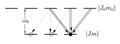
FIG. 1.: Energy representation of a degenerate atomic dipole transition, here for $J=1$, $J_{\mathrm{e}}=2$. Arrows mark atomic transitions from the initial substate, here $|J,m=J\rangle$, under scattering of a photon. In the absence of an external magnetic field, all transitions are elastic. Solid arrows: Rayleigh transitions, conserving the magnetic quantum number ($m^{\prime}=m$). Dotted arrows: degenerate Raman transitions, changing the magnetic quantum number (here $m^{\prime}=m-1$ and $m^{\prime}=m-2$).

In the following, we recall the amplitude for the scattering of one photon by one atom (single scattering) and determine the amplitude for the scattering by two atoms (double scattering). We discuss how the degeneracy of the atomic dipole transition affects the CBS enhancement factor (1). We will use a full quantum mechanical treatment of both atoms and electromagnetic field. While the internal atomic degrees of freedom can only be described quantum mechanically, the electromagnetic field will be described by quantum Fock states for reasons of symmetry. An equivalent treatment can be set up for low-intensity coherent states which are known to correspond closely to a classical light field [29].

Throughout the paper, transitions between identical atomic substates ($m^{\prime}=m$) are called Rayleigh transitions and transitions between different substates ($m^{\prime}\neq m$) are called degenerate Raman transitions. Let us stress that, since one-photon scattering on a degenerate atomic dipole transition is necessarily elastic, inelastic processes (also known as Raman scattering) are completely absent of our analysis. In the following, we use natural units where $\hbar=c=1$ so that $[\mbox{length}]=[\mbox{time}]=[\mbox{frequency}]^{-1}=[\mbox{energy}]^{-1}$.

B Single scattering amplitude

In the single scattering situation, an atom at fixed position ${\bf r}$ is exposed to a plane light wave with wave vector ${\bf k}$, angular frequency $\omega=k$ and transverse polarization $\boldsymbol{\varepsilon}$. We describe the uncoupled system by the sum of the atomic internal hamiltonian and the free field hamiltonian,

$$H_{0}=\omega_{0}\sum_{m_{\mathrm{e}}}|J_{\mathrm{e}}m_{\mathrm{e}}\rangle\langle J_{\mathrm{e}}m_{\mathrm{e}}|+\sum_{{\bf k},\boldsymbol{\varepsilon}\perp{\bf k}}\omega\>a_{{\bf k}\boldsymbol{\varepsilon}}^{\dagger}a_{{\bf k}\boldsymbol{\varepsilon}}.$$ (5)

Here, $a_{{\bf k}\boldsymbol{\varepsilon}}$ and $a_{{\bf k}\boldsymbol{\varepsilon}}^{\dagger}$ are the usual annihilation and creation operator of a transverse field mode with wave vector ${\bf k}$ and polarization vector $\boldsymbol{\varepsilon}$. The corresponding one-photon Fock state will be denoted $|{\bf k}\boldsymbol{\varepsilon}\rangle$ where the transversality $({\bf k}\cdot{\bf\boldsymbol{\varepsilon}})=0$ is understood. The interaction between atom and light is given in the dipole form by $V=-{\bf D}\cdot{\bf E}({\bf r})$. The atomic dipole operator ${\bf D}$ connects the subspaces ${\mathcal{H}}_{J}$ and ${\mathcal{H}}_{J_{\mathrm{e}}}$ (since we consider a closed transition, no other subspaces are involved) with reduced matrix element $\langle J_{\mathrm{e}}||{\bf D}||J\rangle=D\sqrt{2J_{\mathrm{e}}+1}$ [30]. The electric field operator at the atomic position is given by

$${\bf E}({\bf r})=i\sum_{{\bf k},\boldsymbol{\varepsilon}\perp{\bf k}}{\mathcal{E}}_{\omega}\boldsymbol{\varepsilon}_{{\bf k}\boldsymbol{\varepsilon}}a_{{\bf k}\boldsymbol{\varepsilon}}\exp[i({\bf k}\cdot{\bf r})]+h.c.$$ (6)

The field strength ${\mathcal{E}}_{\omega}=(\omega/2\epsilon_{0}L^{3})^{1/2}$ is defined in terms of a quantization volume $L^{3}$ that eventually disappears in results of physical significance.

The probability amplitude for a transition from an initial state $|i\rangle=|{\bf k}\boldsymbol{\varepsilon};Jm\rangle$ to a final state $|f\rangle=|{\bf k}^{\prime}\boldsymbol{\varepsilon}^{\prime};Jm^{\prime}\rangle$ is the element $S_{fi}$ of the scattering matrix. The transition amplitude for $i\neq f$ is written

$$S_{fi}=-2i\pi\delta(\omega-\omega^{\prime})T_{fi}(\omega+i0),$$ (7)

in terms of the transition operator $T$. Here, because the atomic ground state is degenerate, energy conservation, assured by the delta distribution, implies elastic light scattering $(\omega^{\prime}=\omega)$. The matrix element $T_{fi}(z)$ is calculated perturbatively using the Born expansion $T(z)=V+VG_{0}(z)V+\dots$ in powers of the interaction $V$ and the resolvent $G_{0}(z)=(z-H_{0})^{-1}$ of the unperturbed system. The excited atomic state can be eliminated by partial summation of the Born series, dressing the transition frequency and introducing a finite lifetime [27]: $\delta=\omega-\omega_{0}$ is the detuning from the (dressed) transition frequency $\tilde{\omega}_{0}\approx\omega_{0}$ and $\Gamma=D^{2}\omega_{0}^{3}/3\pi\epsilon_{0}$ is the natural width of the atomic excited state.

Let us define the reduced dipole operator ${\bf d}={\bf D}/D$ and the Rabi frequency $\omega_{\mathrm{R}}=D{\mathcal{E}}_{\omega}$. The transition matrix element $T_{fi}=\langle{\bf k}^{\prime}\boldsymbol{\varepsilon}^{\prime},Jm^{\prime}|T(\omega+i0)|{\bf k}\boldsymbol{\varepsilon},Jm\rangle$ near resonance then is

$$T_{fi}=\frac{\omega^{2}_{\mathrm{R}}}{\delta+i\Gamma/2}\langle Jm^{\prime}|(\boldsymbol{\bar{\varepsilon}}^{\prime}\cdot{\bf d})(\boldsymbol{\varepsilon}\cdot{\bf d})|Jm\rangle\;e^{i({\bf k}-{\bf k}^{\prime})\cdot{\bf r}},$$ (8)

represented by its Feynman diagram in fig. 2. The condition “near resonance” means $\delta\ll\omega_{0}$ (but not necessarily $\delta<\Gamma$). Therefore, anti-resonant scattering, i.e., first emission then absorption, can be neglected.

FIG. 2.: Feynman diagram for the transition matrix element $T_{fi}$ (eq. (8)) near resonance. Wavy lines denote photons, straight lines atomic internal states. The thick line stands for the dressed propagator $(\delta+i\Gamma/2)^{-1}$ of the excited atomic state. The absorption vertex yields a factor $\omega_{\mathrm{R}}\exp(i{\bf k}\cdot{\bf r})\langle J_{\mathrm{e}}m_{\mathrm{e}}|\boldsymbol{\varepsilon}\cdot{\bf d}|Jm\rangle$, the emission vertex yields a factor $\omega_{\mathrm{R}}\exp(-i{\bf k}^{\prime}\cdot{\bf r})\langle Jm^{\prime}|\boldsymbol{\bar{\varepsilon}}^{\prime}\cdot{\bf d}|J_{\mathrm{e}}m_{\mathrm{e}}\rangle$, and all intermediate variables, here $m_{\mathrm{e}}$, have to be summed over.

In eq. (8), all information about the atomic internal degrees of freedom and polarization has been factorized into the matrix element

$$\langle Jm^{\prime}|\boldsymbol{\bar{\varepsilon}}^{\prime}\cdot{\bf t}\cdot\boldsymbol{\varepsilon}|Jm\rangle=\frac{\omega^{2}_{\mathrm{R}}}{\delta+i\Gamma/2}\langle Jm^{\prime}|(\boldsymbol{\bar{\varepsilon}}^{\prime}\cdot{\bf d})(\boldsymbol{\varepsilon}\cdot{\bf d})|Jm\rangle.$$ (9)

This defines the scattering operator ${\bf t}$ which acts on the product space ${\mathcal{H}}_{J}\otimes{\mathbb{C}}^{3}$ of atomic internal states and polarizations. It is the scattering operator ${\bf t}$ that characterizes the scattering object and contains all relevant information about the scattering process [31]. We can separate its frequency dependence from its tensor structure: ${\bf t}(\omega)=t(\omega){\bf\hat{t}}$ where

$$t(\omega)=\frac{\omega^{2}_{\mathrm{R}}}{\delta+i\Gamma/2}$$ (10)

is given as the ratio of the squared Rabi frequency (or squared coupling strength) and the resonant denominator known for point dipole scatterers [11]. The novelty of the present approach lies in the peculiar tensor part ${\bf\hat{t}}$. For a given transition $m\rightarrow m^{\prime}$, the dimensionless matrix element

$$\hat{t}_{ij}(m,m^{\prime})=\langle Jm^{\prime}|d_{i}d_{j}|Jm\rangle$$ (11)

defines the scattering tensor which connects the incoming to the outgoing polarization. This $3\times 3$ $t$-matrix can be decomposed into its scalar, antisymmetric and symmetric traceless components, transforming irreducibly under rotations [30].

A classical point dipole scatterer is characterized by a $t$-matrix proportional to unity [11]. This behaviour is reproduced by the elementary dipole transition $J=0$, $J_{\mathrm{e}}=1$. Indeed, the only matrix element of the scattering operator yields the scalar part $\langle 00|\hat{t}_{ij}|00\rangle=\delta_{ij}$. Non-spherical classical scatterers also display an additional traceless symmetric part in their scattering $t$-matrix. In the case of atoms, therefore, it is the antisymmetric part that is characteristic for the quantum internal structure. The antisymmetric part simply implies that an atom scatters light with polarization-dependent strength. To be more specific, consider scattering of circularly polarized light in a Rayleigh transition ($m^{\prime}=m$; quantization axis is the direction of propagation). The scattering strengths for the two possible helicities are different because the Clebsch-Gordan coefficients associated to the transitions $|J,m\rangle\leftrightarrow|J_{\mathrm{e}},m\pm 1\rangle$ are unequal.

This situation is somewhat similar to the usual Faraday effect where circular polarizations with opposite helicities are scattered differently in the presence of an applied magnetic field [32]. There are, however, significant differences: in the Faraday effect, the antisymmetric part of the atomic polarizability depends both on the magnetic field direction and on the direction of light propagation; for the atomic scattering operator, antisymmetry is a fully intrinsic property. When averaged over the internal state, the antisymmetric part of the atomic scattering operator vanishes, leading to a symmetric polarizability and to no dichroism inside the effective medium (cf. Sec. IV A). Thus, the degenerate atomic situation ressembles a (zero magnetic field) Faraday effect depending on the internal state of the atom.

The degeneracy of the atomic ground state also implies that, by scattering a photon, the internal state may change (cf. Fig. 1). The possibility of changing the internal state leaves more choice for the photon polarization. Which polarization is possible for which transition follows from the conservation of angular momentum. In exactly the backscattering direction (${\bf k}^{\prime}=-{\bf k}$) and chosing the quantization axis along the direction of propagation, the following relations hold: linearly polarized light is scattered into the $lin\,{\parallel}\,lin$ channel by a Rayleigh transition ($m^{\prime}=m$), and into the $lin\,{\perp}\,lin$ channel by a degenerate Raman transition ($|m^{\prime}-m|=1$); circularly polarized light is backscattered into the $h\,{\perp}\,h$ channel by Rayleigh transition ($m^{\prime}=m$), and into the $h\,{\parallel}\,h$ channel by a degenerate Raman transition ($|m^{\prime}-m|=2$).

Therefore, the single scattering amplitude shows that changes in the atomic internal state permit changes in the light polarization. Since in general the atomic internal state is not under control, the single backscattering contribution cannot be removed by polarization analysis (with the only exception $J=\frac{1}{2}$ in the $h\,{\parallel}\,h$ channel) and degrades the observable enhancement factor (1).

C Double scattering amplitudes

1 Direct and reverse transition amplitudes

In the double scattering situation, a plane wave impinges upon two atoms $\alpha=1,2$ at fixed positions ${\bf r}_{\alpha}$. The interaction between atoms and field in the full hamiltonian is now $V=-{\bf D}_{1}\cdot{\bf E}({\bf r}_{1})-{\bf D}_{2}\cdot{\bf E}({\bf r}_{2})$. This interaction defines a transition operator $T$ along the lines of Sec. III B. Resonant dipole interaction between the atoms arises from the exchange of photons. Among the numerous different diagrams that describe the transition $|i\rangle=|{\bf k}\boldsymbol{\varepsilon},Jm_{1},Jm_{2}\rangle\rightarrow|f\rangle=|{\bf k}^{\prime}\boldsymbol{\varepsilon}^{\prime},Jm^{\prime}_{1},Jm^{\prime}_{2}\rangle$, the two dominant diagrams involving both atoms are concatenations of two single scattering diagrams. The first diagram, shown in fig. 3, describes the direct scattering path: absorption of the incident photon by atom 1 and emission of the final photon by atom 2. The diagram for the reversed path is obtained by exchanging the role of the two atoms.

FIG. 3.: Feynman diagram of the direct transition matrix element $T_{fi}^{(\mathrm{d}ir)}$ (eq. (12)): resonant scattering first by atom $1$, then by atom $2$. The Feynman rules are defined in fig. 2.

The Feynman rules introduced in fig. 2 permit to explicit the scattering amplitudes. As usual in diagrammatic expansions, a sum over the virtual intermediate states has to be carried out, here the excited atomic states and the intermediate photon. The matrix element for the direct scattering path in the far field approximation $kr_{12}\gg 1$ takes the following form:

$$T^{(\mathrm{d}ir)}_{fi}=-\frac{3\Gamma t^{2}(\omega)}{4\omega^{2}_{\mathrm{R}}}\,\frac{\exp(ikr_{12})}{kr_{12}}\,\hat{t}_{\mathrm{d}ir}\,e^{i({\bf k}\cdot{\bf r}_{1}-{\bf k}^{\prime}\cdot{\bf r}_{2})}.$$ (12)

Again, all information about polarization and internal structure is factorized into the dimensionless matrix element

$$\hat{t}_{\mathrm{d}ir}=\boldsymbol{\bar{\varepsilon}}^{\prime}\cdot{\bf\hat{t}}_{2}(m_{2},m_{2}^{\prime})\cdot\Delta\cdot{\bf\hat{t}}_{1}(m_{1},m_{1}^{\prime})\cdot\boldsymbol{\varepsilon}.$$ (13)

Here, the dimensionless one-atom $t$-matrices, defined in eq. (11), are connected by the projector $\Delta_{ij}=\delta_{ij}-\hat{n}_{i}\hat{n}_{j}$ onto the plane transverse to the unit vector ${\bf\hat{n}}={\bf r}_{12}/r_{12}$ joining the two atoms.

The matrix element $T^{(\mathrm{r}ev)}_{fi}$ for the reversed path is obtained from eq. (12) by exchanging the roles of atoms 1 and 2. The internal matrix element (13) becomes

$$\hat{t}_{\mathrm{r}ev}=\boldsymbol{\bar{\varepsilon}}^{\prime}\cdot{\bf\hat{t}}_{1}(m_{1},m_{1}^{\prime})\cdot\Delta\cdot{\bf\hat{t}}_{2}(m_{2},m_{2}^{\prime})\cdot\boldsymbol{\varepsilon}.$$ (14)

The two amplitudes $T^{(\mathrm{d}ir)}_{fi}$ and $T^{(\mathrm{r}ev)}_{fi}$ describe indistinguishable processes and interfere. A maximal contrast in the backscattering direction is obtained if and only if the amplitudes have equal magnitude $\hat{t}_{\mathrm{d}ir}=\hat{t}_{\mathrm{r}ev}$. But due to the non-scalar part of the atomic $t$-matrix, we expect that in general the matrices do not commute, $\boldsymbol{\hat{t}}_{2}\cdot\Delta\cdot\boldsymbol{\hat{t}}_{1}\neq\boldsymbol{\hat{t}}_{1}\cdot\Delta\cdot\boldsymbol{\hat{t}}_{2}$, so that (13) and (14) are not equal. An exception to this rule is of course the case $m_{1}=m_{2}$, $m_{1}^{\prime}=m_{2}^{\prime}$ where the exchange symmetry assures their equality. Furthermore, we can see that it is precisely the antisymmetric part of the $t$-matrix that is responsible for the inquality of amplitudes in the parallel polarization channels. Indeed, if the one-atom $t$-matrix were symmetric, then $\boldsymbol{\bar{\varepsilon}}^{\prime}\cdot{\bf\hat{t}}_{1}(m_{1},m_{1}^{\prime})\cdot\Delta\cdot{\bf\hat{t}}_{2}(m_{2},m_{2}^{\prime})\cdot\boldsymbol{\varepsilon}=\boldsymbol{\varepsilon}\cdot{\bf\hat{t}}_{2}(m_{2},m_{2}^{\prime})\cdot\Delta\cdot{\bf\hat{t}}_{1}(m_{1},m_{1}^{\prime})\cdot\boldsymbol{\bar{\varepsilon}}^{\prime}$. In the parallel channels $\boldsymbol{\bar{\varepsilon}}^{\prime}=\boldsymbol{\varepsilon}$, from this would immediately follow the equality of the direct and reverse matrix elements (13) and (14). But because of the antisymmetric part of the atomic scattering tensor, in general

$$\begin{split}\boldsymbol{\bar{\varepsilon}}^{\prime}\cdot{\bf\hat{t}}_{1}(m_{1},m_{1}^{\prime})&\cdot\Delta\cdot{\bf\hat{t}}_{2}(m_{2},m_{2}^{\prime})\cdot\boldsymbol{\varepsilon}\neq\\ &\boldsymbol{\varepsilon}\cdot{\bf\hat{t}}_{2}(m_{2},m_{2}^{\prime})\cdot\Delta\cdot{\bf\hat{t}}_{1}(m_{1},m_{1}^{\prime})\cdot\boldsymbol{\bar{\varepsilon}}^{\prime},\end{split}$$ (15)

so that the two interfering amplitudes are different in magnitude. An explicit example for unequal interfering amplitudes in the $h\,{\parallel}\,h$ channel – one is zero while the other is not – has been given in [33].

2 Reciprocity revisited

A question may arise at this point: Does the imbalance of amplitudes $\hat{t}_{\mathrm{d}ir}\neq\hat{t}_{\mathrm{r}ev}$ contradict the theorem of reciprocity? The answer is no: the complete system “field and atoms” obeys reciprocity, but this does not imply $\hat{t}_{\mathrm{d}ir}=\hat{t}_{\mathrm{r}ev}$. The classical reciprocity relation (2) has to be generalized to take into account the set $\{m\}$ of the internal variables of all atoms [34]:

$$\begin{split}T_{\mathrm{d}ir}({\mathbf{k}}\boldsymbol{\varepsilon},\{m\}\rightarrow{\mathbf{k}}^{\prime}\boldsymbol{\varepsilon}^{\prime},\{m^{\prime}\})=(-1)^{\sum_{i}(m_{i}^{\prime}-m_{i})}\\ \times T_{\mathrm{r}ev}(-{\mathbf{k}}^{\prime}{\boldsymbol{\bar{\varepsilon}}^{\prime}},-\{m^{\prime}\}\rightarrow-{\mathbf{k}}\boldsymbol{\bar{\varepsilon}},-\{m\}).\end{split}$$ (16)

This relation shows that in order to obtain the reciprocal sequence of a given sequence, the signs of all internal quantum numbers have to be flipped. The reciprocity relation (16) assures the equality of two interfering CBS amplitudes only if three conditions are met: the two classical conditions (3) on light direction and polarization, and a third one pertaining to the atomic internal variables,

$$\{m^{\prime}\}=\{-m\}.$$ (17)

Whereas the direction of observation and polarization can be controlled experimentally, this is impossible for the internal atomic states in an optically dense medium. Just as in the case of scattering away from the backward direction or into perpendicular polarization channels, reciprocity including the internal states never ceases to be valid, but simply becomes inapplicable to predict the equality of interfering amplitudes. It follows that although there might be some amplitudes satisfying condition (17), the majority will not, and perfect interference contrast is lost. Of course, in the case of the elementary dipole transition $J=0$, $J_{\mathrm{e}}=1$, the condition (17) is trivially fulfilled since all atoms verify $m^{\prime}=m=0$ and we recover the classical case.

Classical reciprocity for light scattering has been derived using Maxwell’s equations for a linear scattering medium provided that its constitutive tensors (dielectric constant, permeablility and conductivity) be symmetric [35]. In the present case, when one does not consider the internal atomic states as intrinsic variables of the system but as given parameters for each path, the $t$-matrix ${\bf\hat{t}}(m,m^{\prime})$ then has an antisymmetric part. In this respect, atoms with degenerate transitions constitute a scattering medium that does not obey classical reciprocity, and a reduced interference is no surprise. Indeed, the same is observed in scattering media with the Faraday effect [36, 37] where the external magnetic field is said to break time-reversal invariance.

Finally, let us note that the ensemble average over the internal variables $\{m\}$ cannot restore the equality of the direct and interference contributions to the diffuse intensity. Indeed, $I_{\mathrm{C}}(0)$ is equal to $I_{\mathrm{L}}$ if and only if, for each pair of scattering paths, the direct and reverse amplitudes are equal. In the sum of all contributions, the equal amplitudes cannot win back what the non-equal amplitudes have lost: the result is a reduced overall enhancement factor.

3 The role of degenerate Raman transitions

In the case of the elementary dipole transition $J=0$, $J_{\mathrm{e}}=1$, the atomic scattering tensor only has a scalar part $\langle 00|\hat{t}_{ij}|00\rangle=\delta_{ij}$. The analysis of the double scattering amplitudes in Sec. III C 1 shows that the internal amplitudes then are equal and full interference contrast is guaranteed. As for $J=0$ no degenerate Raman transitions ($m^{\prime}\neq m$) can occur, the following question is inevitable: can the decrease of interference contrast be attributed to the Raman transitions alone?

Indeed, one might be tempted to suggest incoherence of the Raman scattered light (i.e., the loss of phase coherence in spontaneous emission) as the origin for this loss of contrast. In the present description, however, this is not a pertinent explanation. It is true that the Raman scattered light does not interfere with the reference light from the source: the respective final atomic states are orthogonal and the two amplitudes do not describe indistinguishable processes (this is a typical “which-path” argument [38, 39]). But a photon scattered elastically along the direct path interferes very well with the same photon scattered along the reverse path — as long as the internal states of all atoms in both processes are identical, no matter whether they describe degenerate Raman or Rayleigh transitions.

A closer analysis of the situation in the channels of circular polarization permits the following remarks. In the channel $h\,{\perp}\,h$ of flipped helicity, a selection rule special to the double scattering configuration admits only Rayleigh transitions to the crossed intensity. The ladder intensity contains a contribution from Rayleigh transitions (equal to the crossed intensity) and an additional contribution from degenerate Raman transitions. In this sense, the degenerate Raman transitions are responsible for a reduced double scattering interference in the $h\,{\perp}\,h$ channel. This is consistent with the observation that degenerate Raman transitions make the atoms behave as non-spherical scatterers for which reduced interference in the perpendicular channels is expected. But for higher scattering orders, Raman transitions contribute also to the crossed intensity, and it is no longer evident to compare the relative weights of Rayleigh and Raman contributions.

The explicit example of a double Rayleigh transition in the $h\,{\parallel}\,h$ channel with zero interference given in ref. [33], shows that Rayleigh transitions also are responsible for a loss of contrast. On the other hand, the fact that Raman transitions give to atoms some characteristics of non-spherical scatterers does not by itself imply a loss of contrast: the reciprocity theorem is independent of the actual shape of the scatterers and applies to spherical as well as to non-spherical classical scatterers. For example, a double Raman transition such that ($m_{1}=m_{2}=-m_{1}^{\prime}=-m_{2}^{\prime}\neq 0$) satisfies the reciprocity condition (17) and has perfect contrast (as is also evident from the exchange symmetry). In the sum of all scattering amplitudes, Raman scattering amplitudes can even be dominant in the backscattering interference signal. An explicit example of such a situation is given in fig. 9.

In fact, independently of the scattering order, it is precisely the antisymmetric part of the atomic scattering tensor that is responsible for the loss of contrast in the parallel polarization channels. This antisymmetric part appears for both degenerate Raman and Rayleigh transitions (cf. the unequal scattering of circularly polarized light with different helicities as mentioned in Sec. III B). Therefore, the degenerate Raman transitions must not be held responsible alone for the reduction of interference contrast.

IV Analytical formulation of the internal ensemble average

We wish to describe the light propagation inside a macroscopic disordered medium on average. Starting from an entirely symmetric microscopic description of matter and light, the ensemble average is a trace over the matter degrees of freedom. This trace contains an average over atomic positions as well as an average over the internal degrees of freedom. This is analogous to the case of classical non-spherical scatterers where averages over position and orientation have to be performed. We suppose in the following that the atomic sample is prepared without correlations between positions and internal substates, and that different atoms are uncorrelated. This is a reasonable assumption for a cloud of cold atoms created from a standard magneto-optical trap. The two averaging procedures then become independent. As far as positions are concerned, we will use the averaging techniques developed for classical point scatterers [3]. In the independent scattering approximation, the average over the internal quantum numbers $\{m\}$ can be expressed as traces over a one-atom density matrix $\rho$ and one-atom operators.

A Average amplitudes: effective medium

Tracing over the matter degrees of freedom defines an effective medium for the average propagation of light amplitudes and intensities. In this paragraph, we will deal with the rather simple issue of the average amplitude. As will be seen, the internal structure of the atomic scatterers provides no major surprise, and we are able to recover the well-known properties of a dilute atomic gas [29]. The impact of the effective medium on the amplitude is described by the self-energy $\Sigma(\omega)$ that renormalizes the vacuum light frequency $\omega$ [11]. In the independent scattering approximation, the self-energy is proportional to the average scattering operator,

$$\boldsymbol{\Sigma}(\omega)=N{\mathrm{T}r}\rho{\bf t}(\omega)=N\left\langle{\mathbf{t}}(\omega)\right\rangle_{\mathrm{i}nt}.$$ (18)

Because of the vector character of the light wave, the self-energy is formally a second rank tensor. Assuming a scalar density matrix, i.e., a uniform distribution over internal states, the internal average simply projects onto the scalar part: $\boldsymbol{\Sigma}(\omega)=\Sigma(\omega)\boldsymbol{1}$. Calculating the average is elementary using the closure relation of Clebsch-Gordan coefficients, and we find

$$\Sigma(\omega)=nM_{J}\frac{3\pi}{\omega^{2}}\frac{\Gamma/2}{\delta+i\Gamma/2}$$ (19)

Here, we define for convenience the ratio of multiplicities

$$M_{J}=\frac{2J_{\mathrm{e}}+1}{3(2J+1)}$$ (20)

with $M_{0}=1$. The atomic polarizability close to resonance is given by

$$\boldsymbol{\alpha}(\omega)=-\frac{2L^{3}}{\omega}\left\langle{\mathbf{t}}(\omega)\right\rangle_{\mathrm{i}nt}.$$ (21)

Expliciting the internal average as a weighted sum over substates,

$$\left\langle{\bf t}(\omega)\right\rangle_{\mathrm{i}nt}=\sum_{m}p_{m}\langle Jm|{\bf t}(\omega)|Jm\rangle,$$ (22)

it is evident that solely the Rayleigh transitions $(m^{\prime}=m)$ enter into the definition of the self-energy and of the polarizability. In the case of a uniform distribution with weights $p_{m}=(2J+1)^{-1}$, this average selects the scalar part of the scattering operator. A thorough discussion of the polarizability, the scattering operator and its analysis by decomposition in irreducible components can be found in the textbook by Berestetskii et al. [31].

The susceptibility of the dilute atomic medium is $\chi=n\alpha$, and the condition of low density now reads $n\alpha\ll 1$. The effective refractive index then is given by $n_{\mathrm{r}}=1+n\alpha/2$. Its real part is very close to unity, and we need not distinguish between the optical wavelength in the medium and in the vacuum. Its imaginary part describes attenuation of the average amplitude, and here the effect of the dilute medium is essential. Since we do not describe any absorption, all attenuation is necessarily due to scattering from the initial mode into other modes. This argument is the essence of the optical theorem

$$\sigma_{\mathrm{t}ot}=-2L^{3}{\mathrm{I}m}\left\langle\boldsymbol{\bar{\varepsilon}}\cdot{\bf t}(\omega)\cdot\boldsymbol{\varepsilon}\right\rangle_{\mathrm{i}nt}=k\ {\mathrm{I}m}\alpha(\omega).$$ (23)

We thus find the total scattering cross-section

$$\sigma_{\mathrm{t}ot}=M_{J}\frac{6\pi}{k^{2}}\frac{1}{1+4\delta^{2}/\Gamma^{2}}.$$ (24)

This well known expression features the resonant dipole cross-section $6\pi/k^{2}=3\lambda^{2}/2\pi$ and the Lorentzian line shape for detuning $\delta$ around the resonance with width $\Gamma$.

The mean free path of the light inside the average medium is $\ell=-2({\mathrm{I}m}\Sigma(\omega))^{-1}$. By virtue of the optical theorem, it depends on the total cross-section and on the number density of scatterers through:

$$\ell=\frac{1}{n\sigma_{\mathrm{t}ot}}$$ (25)

and is independent of both the polarization and the direction of propagation. This reflects statistical invariance of the atomic medium under rotation.

In summary, in the weak density and weak scattering regime, the internal structure has very small influence on the properties of an average light amplitude. For a uniform statistical distibution over internal states, all average quantities are isotropic and are only modified by a factor $M_{J}=(2J_{\mathrm{e}}+1)/3(2J+1)$ with respect to the classical dipole point scatterer where $M_{0}=1$. This is not surprising since the internal average over a scalar density matrix simply selects the scalar part of the atomic scattering operator. The antisymmetric part that appeared as the genuine quantum feature in Sec. III therefore is not present here.

B Average intensities

Coherent backscattering is an interference effect for the average intensity, which of course must be distinguished from the square of the average amplitude. Consequently, we stress that it is not sufficient to calculate quantities pertaining to the average amplitude (such as the polarizability or the scattering mean free path) in order to decide whether the internal structure affects CBS or localization. In the following paragraphs, we show how proper use of tensor algebra makes it possible to analytically perform the averaging over the atomic internal degrees of freedom. In the specific case of a semi-infinite medium, exact averaging over the external position of the atoms is also possible for the single and double scattering contributions.

The average scattered intensity $I$ far away from the medium can be calculated in terms of the dimensionless bistatic coefficient [40]

$$\gamma=\frac{4\pi}{A}\left\langle\frac{d\sigma}{d\Omega}({\bf k}\boldsymbol{\varepsilon}\rightarrow{\bf k}^{\prime}\boldsymbol{\varepsilon}^{\prime})\right\rangle.$$ (26)

Here, the light incidence is supposed to be perpendicular to the surface $A$ of the medium which will be taken to become the half space $z>0$ as $A\rightarrow\infty$. The average differential cross section is determined by Fermi’s golden rule which reads

$$\left\langle\frac{d\sigma}{d\Omega}({\bf k}\boldsymbol{\varepsilon}\rightarrow{\bf k}^{\prime}\boldsymbol{\varepsilon}^{\prime})\right\rangle=\frac{L^{6}\omega^{2}}{4\pi^{2}}\left\langle|T({\bf k}^{\prime}\boldsymbol{\varepsilon}^{\prime},{\bf k}\boldsymbol{\varepsilon})|^{2}\right\rangle.$$ (27)

The square of the transition operator means explicitly $|T({\bf k}^{\prime}\boldsymbol{\varepsilon}^{\prime},{\bf k}\boldsymbol{\varepsilon})|^{2}=\langle{\bf k}\boldsymbol{\varepsilon}|T(\omega+i0)^{\dagger}|{\bf k}^{\prime}\boldsymbol{\varepsilon}^{\prime}\rangle\langle{\bf k}^{\prime}\boldsymbol{\varepsilon}^{\prime}|T(\omega+i0)|{\bf k}\boldsymbol{\varepsilon}\rangle$ and acts on the atomic states only. Note that the factor $L^{6}$ cancels with the inverse factor coming from the squared transition operator, so that the quantization volume finally disappears.

For single scattering, eqs. (8) and (9) show that the internal average has to be taken over the square of the (dimensionless) scattering operator:

$$\left\langle|\boldsymbol{\bar{\varepsilon}}^{\prime}\cdot{\bf\hat{t}}\cdot\boldsymbol{\varepsilon}|^{2}\right\rangle_{\mathrm{i}nt}={\mathrm{T}r}[\rho(\boldsymbol{\bar{\varepsilon}}\cdot{\bf d})(\boldsymbol{\varepsilon}^{\prime}\cdot{\bf d})(\boldsymbol{\bar{\varepsilon}}^{\prime}\cdot{\bf d})(\boldsymbol{\varepsilon}\cdot{\bf d})].$$ (28)

It is crucial that the average be taken over the square of the scattering tensor. This is not equivalent to taking the square of the average which is essentially the polarizability (21). Again, the trace over a scalar density matrix will select the scalar part of the averaged operator. But, as becomes evident in App. A, now the antisymmetric and symmetric traceless parts can combine with their counterpart in the direct product and contribute a non-trivial scalar component.

In the double scattering situation, the two atoms are coupled by the intermediate photon. Let

$$\hat{t}_{21}=\boldsymbol{\bar{\varepsilon}}^{\prime}\cdot{\bf\hat{t}}_{2}\cdot\Delta\cdot{\bf\hat{t}}_{1}\cdot\boldsymbol{\varepsilon}$$ (29)

be a short-hand notation for the contracted double scattering operator for the direct path, and $\hat{t}_{12}$ for the reverse path. The ladder contribution to the double scattering intensity, just like in the classical case, is given by the average sum of the squares of the two amplitudes,

$${{\mathrm{T}r}}[\rho_{12}(|\hat{t}_{21}|^{2}+|\hat{t}_{12}|^{2})].$$ (30)

Here, $\rho_{12}$ is the two-scatterer density matrix. The crossed contribution is obtained, again in perfect analogy to the classical case, by the interference between the direct and reverse amplitude

$${\mathrm{T}r}[\rho_{12}(\hat{t}_{12}\bar{\hat{t}}_{21}\exp[i({\bf k}+{\bf k}^{\prime})\cdot{\bf r}_{12}]+(1\leftrightarrow 2))].$$ (31)

Since the atoms are uncorrelated, the density matrix factorizes, $\rho_{12}=\rho_{1}\otimes\rho_{2}$. Furthermore, $\rho_{\alpha}=\rho$ since the atoms are identically distributed. The two-atom scattering operator (29) is not factorized in terms of elementary scalar products. But by expliciting the transverse projector $\Delta_{ij}=\delta_{ij}-\hat{n}_{i}\hat{n}_{j}$, it becomes

$$\hat{t}_{21}=(\boldsymbol{\bar{\varepsilon}}^{\prime}\cdot{\bf d}_{2})[({\bf d}_{2}\cdot{\bf d}_{1})-({\bf\hat{n}}\cdot{\bf d}_{2})({\bf\hat{n}}\cdot{\bf d}_{1})](\boldsymbol{\varepsilon}\cdot{\bf d}_{1}).$$ (32)

All averages (28), (30) and (31) can then be expressed as linear combinations of the one-atom trace

$\displaystyle{\mathrm{T}r}[\rho({\bf x}_{4}\cdot{\bf d})({\bf x}_{3}\cdot{\bf d})({\bf x}_{2}\cdot{\bf d})({\bf x}_{1}\cdot{\bf d})]$

where the fixed vectors ${\bf x}_{\alpha}$ stand for $\boldsymbol{\varepsilon},\boldsymbol{\bar{\varepsilon}},\boldsymbol{\varepsilon}^{\prime},\boldsymbol{\bar{\varepsilon}}^{\prime},{\bf\hat{n}},$ or ${\bf d}^{\prime}$ (the dipole operator of the other atom). Rather than calculating each term separately, we determine the one-atom trace for four arbitray ${\bf x}_{\alpha}$ and later substitute what is required by the single and double scattering terms.

C The single scattering vertex

We proceed to calculate the dimensionless trace function

$${\mathcal{T}}({\bf x}_{\alpha})=\frac{1}{M_{J}}{{\mathrm{T}r}}[\rho({\bf x}_{4}\cdot{\bf d})({\bf x}_{3}\cdot{\bf d})({\bf x}_{2}\cdot{\bf d})({\bf x}_{1}\cdot{\bf d})].$$ (33)

It depends linearly on the components of the ${\bf x}_{\alpha}$, albeit in a complicated manner, involving the characteristics of the transition and the elements of the density matrix. A systematic way of evaluating the trace is a development in terms transforming under irreducible representations of the rotation group [41]. We shall explicit the solution in the simplest case when the atom is distributed with equal probability over its internal substates. Since the corresponding density matrix is then proportional to unity and therefore a scalar under rotations, the trace selects the scalar part of the averaged operator. The result can only be a function of the scalar products $({\bf x}_{\alpha}\cdot{\bf x}_{\beta})$, of the most general form

$$\begin{split}{\mathcal{T}}({\bf x}_{\alpha})&=w_{1}({\bf x}_{1}\cdot{\bf x}_{2})({\bf x}_{3}\cdot{\bf x}_{4})+w_{2}({\bf x}_{1}\cdot{\bf x}_{3})({\bf x}_{2}\cdot{\bf x}_{4})\\ &\quad+w_{3}({\bf x}_{1}\cdot{\bf x}_{4})({\bf x}_{2}\cdot{\bf x}_{3}).\end{split}$$ (34)

The coefficients $w_{i}$ are calculated explicitly using the standard techniques of irreducible tensor operators (details are given in appendix A):

$$w_{1}=\frac{s_{0}-s_{2}}{3},\ w_{2}=\frac{s_{2}-s_{1}}{2},\ w_{3}=\frac{s_{1}+s_{2}}{2}$$ (35)

where

$$s_{K}=3(2J_{\mathrm{e}}+1)\left\{\begin{array}[]{ccc}1&1&K\\ J&J&J_{\mathrm{e}}\end{array}\right\}^{2}.$$ (36)

The “$6J$”-symbols [30] (or Wigner coupling coefficients) contain all essential informations about our problem. They are the simplest scalar quantities that can be constructed from the basic ingredients $J$, $J_{\mathrm{e}}$, $1$ (the rank of the vector operator ${\bf d}$) and $K$ (the tensor ranks of the irreducible components of the scattering operator). The “$6J$”-symbols introduce useful selection rules:

1. $|J-J_{\mathrm{e}}|\leq 1$, the usual selection rule for a dipole transition;

2. $0\leq K\leq 2$: the scattering operator is the direct product of two vector operators and thus has irreducible components of rank $K=0,1,2$. In other words, the change of the atomic angular momentum is limited to $|m^{\prime}-m|\leq 2$ for the one photon scattering;

3. $K\leq 2J$: the ground state degeneracy determines which tensor rank comes into play. For $J=0$, $K=0$ and thus only Rayleigh transitions $m^{\prime}-m=0$ are possible; for $J=1/2$, $K=0,1$ and degenerate Raman transitions with $|m^{\prime}-m|=1$ become possible; for $J\geq 1$, $K=0,1,2$ and all possible transitions $|m^{\prime}-m|\leq 2$ can take place.

A sum rule over $K$ for the “$6J$”-symbols implies that the $w$ coefficients are not independent but obey

$$w_{1}+w_{2}+3w_{3}=1$$ (37)

for arbitrary $J,J_{\mathrm{e}}$. Explicit formulae for the $w_{i}$ are contained in app. B 1.

We introduce a diagrammatical representation for the trace function (34):

$$\vertex{{\bf x}_{1}}{{\bf x}_{2}}{{\bf x}_{3}}{{\bf x}_{4}}=w_{1}\horizontal{1\,}{\,2}{\,3}{4\,}+w_{2}\diagonal{1}{\,2}{\,3}{4}+w_{3}\vertical{1}{2}{3}{4}$$ (38)

This four-point intensity vertex is the weighted sum of the three pairwise contractions between the vectors ${\bf x}_{\alpha}$. A factor $w_{1}$ comes in for the horizontal pairwise contraction $({\bf x}_{1}\cdot{\bf x}_{2})({\bf x}_{3}\cdot{\bf x}_{4})$, a factor $w_{2}$ for a diagonal pairwise contraction, and a factor $w_{3}$ for a vertical pairwise contraction. It ressembles Wicks’s theorem known from Gaussian integration [42], but here, the weights of the possible contractions are not equal. As in quantum field theory, this diagrammatic representation proves especially useful for the systematic description of higher-order scattering (cf. Sec. IV E).

D The single scattering contribution

Using $\boldsymbol{\varepsilon}=\bar{\bf x}_{1}={\bf x}_{4}$ and $\boldsymbol{\varepsilon}^{\prime}={\bf x}_{2}=\bar{\bf x}_{3}$ in (34), the internal average (28) for the single scattering contribution becomes

$$\left\langle|\boldsymbol{\bar{\varepsilon}}^{\prime}\cdot{\bf\hat{t}}\cdot\boldsymbol{\varepsilon}|^{2}\right\rangle_{\mathrm{i}nt}=M_{J}\left(w_{1}|\boldsymbol{\bar{\varepsilon}}^{\prime}\cdot\boldsymbol{\varepsilon}|^{2}+w_{2}|\boldsymbol{\varepsilon}^{\prime}\cdot\boldsymbol{\varepsilon}|^{2}+w_{3}\right)$$ (39)

The average differential cross-section for single scattering on an unpolarized atom is

$$\left\langle\frac{d\sigma_{\mathrm{S}}}{d\Omega}\right\rangle_{\!\!\mathrm{i}nt}=\frac{3\sigma_{\mathrm{t}ot}}{8\pi}\left(w_{1}|\boldsymbol{\bar{\varepsilon}}^{\prime}\cdot\boldsymbol{\varepsilon}|^{2}+w_{2}|\boldsymbol{\varepsilon}^{\prime}\cdot\boldsymbol{\varepsilon}|^{2}+w_{3}\right)$$ (40)

in terms of the total scattering cross-section (24). Using this expression, we see that the sum rule (37) simply represents flux conservation. All angular information is contained in the squared moduli of polarization contractions. Since these expressions are even in the scattering angle $\theta$, the mean value $\left\langle\cos\theta\right\rangle=\int d\theta\left\langle d\sigma/d\Omega\right\rangle\cos\theta$ vanishes, justifying that the transport mean free path $\ell_{\mathrm{tr}}=\ell/(1-\left\langle\cos\theta\right\rangle)$ is equal to the scattering mean free path $\ell$.

To determine the bistatic coefficient now means to average eq. (40) over position. We assume a semi-infinite, homogenous medium of independently distributed atoms. The single scattering bistatic coefficient then is

$$\gamma_{\mathrm{S}}=\frac{4\pi n}{A}\int_{z>0}\!\!\!\!\!\!\!d^{3}{r}\;\left\langle\frac{d\sigma_{\mathrm{S}}}{d\Omega}\right\rangle_{\!\!\mathrm{i}nt}e^{-2z/\ell}.$$ (41)

The exponential takes account of the extinction of incoming and scattered light with the mean free path $\ell$ inside the scattering medium. Since the differential cross-section is independent of the position, the integral is readily calculated and we find

$$\gamma_{\mathrm{S}}=\frac{3}{4}\ \vertex{\boldsymbol{\varepsilon}}{\boldsymbol{\bar{\varepsilon}}^{\prime}}{\boldsymbol{\varepsilon}^{\prime}}{\boldsymbol{\bar{\varepsilon}}}=\frac{3}{4}\left(w_{1}|\boldsymbol{\bar{\varepsilon}}^{\prime}\cdot\boldsymbol{\varepsilon}|^{2}+w_{2}|\boldsymbol{\varepsilon}^{\prime}\cdot\boldsymbol{\varepsilon}|^{2}+w_{3}\right).$$ (42)

The coefficients $w_{i}(J,J_{\mathrm{e}})$ carry the weights of the different contractions of the polarization vectors (for detailed expressions, see app. B 1). In the case of a transition $J=0$, $J_{\mathrm{e}}=1$, these coefficients are simply $(w_{1},w_{2},w_{3})=(1,0,0)$. So one recovers exactly the classical expression [43]

$$\gamma_{\mathrm{S}}=\frac{3}{4}\clvertex{\boldsymbol{\varepsilon}}{\boldsymbol{\bar{\varepsilon}}^{\prime}}{\boldsymbol{\varepsilon}^{\prime}}{\boldsymbol{\bar{\varepsilon}}}=\frac{3}{4}|\boldsymbol{\bar{\varepsilon}}^{\prime}\cdot\boldsymbol{\varepsilon}|^{2}.$$ (43)

In the classical diagram, the upper line, read from left to right, signifies scattering of the wave amplitude, and the lower line, read from right to left, signifies scattering of the complex conjugate amplitude by the same scatterer (identified by the dashed line). The only possible connection is horizontal, giving the factor $|\boldsymbol{\bar{\varepsilon}}^{\prime}\cdot\boldsymbol{\varepsilon}|^{2}$ that implies a dipole radiation pattern. For atoms, however, the coefficients $w_{2}$ and $w_{3}$ come into play and lead to contributions in the $lin\,{\perp}\,lin$ channel (where $\boldsymbol{\bar{\varepsilon}}^{\prime}\cdot\boldsymbol{\varepsilon}=\boldsymbol{\varepsilon}^{\prime}\cdot\boldsymbol{\varepsilon}=0$) as soon as $J\geq 1/2$. When $J\geq 1$, there is a signal even in the helicity preserving backscattering channel $h\,{\parallel}\,h$ (where $\boldsymbol{\bar{\varepsilon}}^{\prime}\cdot\boldsymbol{\varepsilon}=0$, $\boldsymbol{\varepsilon}^{\prime}\cdot\boldsymbol{\varepsilon}=1$). Now we see why the polarizability (21) is not sufficient to describe the scattering by a degenerate transition. The polarizability is essentially the average scattering tensor, a two-point vertex connecting the incoming to the outgoing polarization. If the atom is distributed with equal probability over its substates, the polarizability then is diagonal and defines a purely horizontal contraction proportional to $|\boldsymbol{\bar{\varepsilon}}^{\prime}\cdot\boldsymbol{\varepsilon}|^{2}$. But the internal structure of an atom allows also for diagonal and vertical connections in the single scattering diagram: the classical line stretches to a two dimensional ribbon.

E The double scattering contributions

Van Tiggelen et al. [43] have calculated the double-scattering contribution to the ladder bistatic coefficient in the backward direction,

$$\gamma_{\mathrm{L}2}=\frac{9}{16\pi A\ell^{2}}\int_{z_{1,2}>0}\!\!\!\!\!\!\!\!\!d^{3}{r}_{1}d^{3}{r}_{2}\;\;\frac{e^{-(z_{1}+r_{12}+z_{2})/\ell}}{r_{12}^{2}}\>P_{\mathrm{L}2}$$ (44)

for classical point scatterers in a half-space, within the weak scattering limit $k\ell\gg 1$ and in the far field approximation $kr_{12}\gg 1$. Here, the exponential describes the attenuation of incident, intermediate and scattered light with mean free path $\ell$. For classical dipole point scatterers, the polarization kernel is given by $P_{\mathrm{L}2}^{(\mathrm{cl})}=|\boldsymbol{\bar{\varepsilon}}^{\prime}\cdot\Delta\cdot\boldsymbol{\varepsilon}|^{2}$. For atomic scatterers under the same conditions, eq. (44) remains valid. As all information about the internal structure is connected to the polarization, only the polarization kernel has to be generalized. Keeping track of all factors, it follows from Sec. IV B that the polarization kernel is given as the internal average (30) over the square of the dimensionless double scattering operator:

$$P_{\mathrm{L}2}=M_{J}^{-2}\left\langle|\boldsymbol{\bar{\varepsilon}}^{\prime}\cdot{\bf\hat{t}}_{2}\cdot\Delta\cdot{\bf\hat{t}}_{1}\cdot\boldsymbol{\varepsilon}|^{2}\right\rangle_{\mathrm{i}nt}.$$ (45)

Using eqs. (29) to (38), it is represented by the generalized ladder diagram

$$P_{\mathrm{L}2}=\doubleladder{\boldsymbol{\varepsilon}}{\boldsymbol{\bar{\varepsilon}}^{\prime}}{\boldsymbol{\varepsilon}^{\prime}}{\boldsymbol{\bar{\varepsilon}}}.$$ (46)

This double-scattering ladder diagram is the product of two single scattering diagrams (38) connected by the polarization propagator $\Delta_{ij}=\delta_{ij}-\hat{n}_{i}\hat{n}_{j}$, one for the amplitude (upper line) and one for its complex conjugate (lower line). The diagram is evaluated using the following rules. Each scattering box yields three pairwise contractions: horizontal with weight $w_{1}$, diagonal with weight $w_{2}$ and vertical with weight $w_{3}$. Now choose $w_{i}w_{j}$ for the two boxes and contract the vectors accordingly. For example, $w_{1}^{2}$ comes with the twofold horizontal contraction $|\boldsymbol{\varepsilon}\cdot\Delta\cdot\boldsymbol{\bar{\varepsilon}}^{\prime}|^{2}$; $w_{1}w_{2}$ and $w_{2}w_{1}$ both give $|\boldsymbol{\varepsilon}\cdot\Delta\cdot\boldsymbol{\varepsilon}^{\prime}|^{2}$. For the vertical connections involving factors of $w_{3}$, one has to use that the polarization propagator is a projector, $\Delta\cdot\Delta=\Delta$, and its total contraction (arising for $w_{3}^{2}$) is $\sum_{i}\Delta_{ii}=2$. Finally

$$\begin{split}P_{\mathrm{L}2}&=(w_{1}^{2}+w_{2}^{2})|\boldsymbol{\bar{\varepsilon}}^{\prime}\cdot\Delta\cdot\boldsymbol{\varepsilon}|^{2}+2w_{1}w_{2}|\boldsymbol{\varepsilon}^{\prime}\cdot\Delta\cdot\boldsymbol{\varepsilon}|^{2}\\ &\quad+(w_{1}+w_{2})w_{3}[(\boldsymbol{\bar{\varepsilon}}\cdot\Delta\cdot\boldsymbol{\varepsilon})+(\boldsymbol{\bar{\varepsilon}}^{\prime}\cdot\Delta\cdot\boldsymbol{\varepsilon}^{\prime})]+2w_{3}^{2}\end{split}$$ (47)

For classical dipole scatterers, modeled by a transition $J=0$, $J_{\mathrm{e}}=1$, one has $(w_{1},w_{2},w_{3})=(1,0,0)$ and recovers the known result

$$P_{\mathrm{L}2}^{(\mathrm{cl})}=\cldoubleladder{\boldsymbol{\varepsilon}}{\boldsymbol{\bar{\varepsilon}}^{\prime}}{\boldsymbol{\varepsilon}^{\prime}}{\boldsymbol{\bar{\varepsilon}}}=|\boldsymbol{\bar{\varepsilon}}^{\prime}\cdot\Delta\cdot\boldsymbol{\varepsilon}|^{2}.$$ (48)

The crossed bistatic coefficient for the double-scattering contribution as calculated by van Tiggelen et al. [43] under the same assumptions is

$$\begin{split}\gamma_{\mathrm{C}2}=\frac{9}{16\pi A\ell^{2}}\int_{z_{1,2}>0}\!\!\!\!\!\!\!\!d^{3}{r}_{1}d^{3}{r}_{2}&\;\frac{e^{-(sz_{1}+r_{12}+sz_{2})/\ell}}{r_{12}^{2}}\\ &\times\cos[({\bf k}+{\bf k}^{\prime})\cdot{\bf r}_{12}]\;P_{\mathrm{C}2}\end{split}$$ (49)

where $s=\frac{1}{2}(1+1/\cos\theta)$. For classical dipole point scatterers, the crossed and ladder polarization kernels are equal, $P_{\mathrm{C}2}^{(\mathrm{cl})}=P_{\mathrm{L}2}^{(\mathrm{cl})}$. This assures that in the backscattering direction ($\theta=0$, ${\bf k}^{\prime}=-{\bf k}$), crossed and ladder intensities are equal (the strict equality for all polarizations is characteristic of double scattering; for higher scattering orders, equality of crossed and ladder is only given for parallel polarizations). In the case of atomic scatterers, eq. (49) remains valid, but the polarization kernel has to be generalized. Casting the internal average (31) in diagrammatical form, it is

$$P_{\mathrm{C}2}=\doublecrossed{\boldsymbol{\varepsilon}}{\boldsymbol{\bar{\varepsilon}}^{\prime}}{\boldsymbol{\varepsilon}^{\prime}}{\boldsymbol{\bar{\varepsilon}}}\quad.$$ (50)

The crossed diagram is evaluated efficiently using the contraction rules defined above for the ladder diagram. Explicitly,

$$\begin{split}P_{\mathrm{C}2}&=(w_{1}^{2}+w_{3}^{2})|\boldsymbol{\bar{\varepsilon}}^{\prime}\cdot\Delta\cdot\boldsymbol{\varepsilon}|^{2}+2w_{1}w_{3}(\boldsymbol{\bar{\varepsilon}}^{\prime}\cdot\Delta\cdot\boldsymbol{\varepsilon}^{\prime})(\boldsymbol{\varepsilon}\cdot\Delta\cdot\boldsymbol{\bar{\varepsilon}})\\ &+(w_{1}+w_{3})w_{2}[(\boldsymbol{\varepsilon}\cdot\boldsymbol{\varepsilon}^{\prime})(\boldsymbol{\bar{\varepsilon}}\cdot\Delta\cdot\boldsymbol{\bar{\varepsilon}}^{\prime})+(\boldsymbol{\bar{\varepsilon}}\cdot\boldsymbol{\bar{\varepsilon}}^{\prime})(\boldsymbol{\varepsilon}\cdot\Delta\cdot\boldsymbol{\varepsilon}^{\prime})]\\ &+2w_{2}^{2}|\boldsymbol{\varepsilon}^{\prime}\cdot\boldsymbol{\varepsilon}|^{2}\end{split}$$ (51)

Obviously, the crossed kernel is not equal to the ladder kernel, $P_{\mathrm{C}2}\neq P_{\mathrm{L}2}$. What is the relation between the two? In the classical theory, one habitually uses time reversal invariance to reduce one to the other: returning the lower line of the crossed diagram for classical point scatterers

$$P_{\mathrm{C}2}^{(\mathrm{cl})}=\cldoublecrossed{\boldsymbol{\varepsilon}}{\boldsymbol{\bar{\varepsilon}}^{\prime}}{\boldsymbol{\varepsilon}^{\prime}}{\boldsymbol{\bar{\varepsilon}}}\quad,$$ (52)

the connecting lines are straightened out, and the crossed diagram becomes equal to the ladder diagram (48) in the parallel polarization channels $\boldsymbol{\bar{\varepsilon}}^{\prime}=\boldsymbol{\varepsilon}$. This is the signature of reciprocity and assure a perfect interference contrast in the backscattering direction. But returning the bottom line of the generalized crossed diagram (50), we find

$$P_{\mathrm{C}2}=\twisteddoublecrossed{\boldsymbol{\varepsilon}}{\boldsymbol{\bar{\varepsilon}}^{\prime}}{\boldsymbol{\bar{\varepsilon}}}{\boldsymbol{\varepsilon}^{\prime}}$$ (53)

which differs from the ladder diagram (46), even if we put $\boldsymbol{\bar{\varepsilon}}^{\prime}=\boldsymbol{\varepsilon}$. What has happened? The ribbon that has replaced the classical line cannot unwind and blocks the diagram topologically. It blocks because the diagonal and the vertical contraction are not equivalent: $w_{2}\neq w_{3}$. Only in the case $J=0$, $J_{\mathrm{e}}=1$, we have $w_{2}=w_{3}=0$, and one recovers the correspondence to the classical point dipole scatterers. Eq. (35) shows that $w_{2}=w_{3}$ if and only if $s_{1}=0$. The coefficient $s_{1}$ stems from the antisymmetric part of the scattering operator (cf. app. A). As the analysis of the double scattering amplitude in Sec. III C already showed, it is the antisymmetric part of the atomic scattering operator that is responsible for the reduction of the backscattering enhancement in the parallel channels.

V Enhancement factors and peak analysis for any atomic transition

The results of the previous section enable us to calculate analytically the intensity of polarized light scattered at first and second order by atoms which are positioned randomly in a half-space. The spatial integrals in eqs. (44) and (49) are challenging because of the half-space geometry, but can be performed fully analytically – see section B 3. We therefore obtain the various enhancement factors at backscattering as well as the shape of the backscattered cone fully analytically. In this section, we analyze the contributions of single and double scattering to the backscattered intensity and determine the second-order enhancement factor as a function of the polarization channel and the atomic dipole transition.

A Single scattering background

The single scattering intensity in terms of the bistatic coefficient $\gamma_{\mathrm{S}}$ is given by eq. (42) as a function of the ground state angular momentum $J$, the transition type $J_{\mathrm{e}}-J=0,\pm 1$ and the polarization vectors. Fig. 4 shows $\gamma_{\mathrm{S}}$ for all transition types and the four standard polarization configurations.

FIG. 4.: Single scattering intensity in terms of the bistatic coefficient (42) in the backscattering direction as a function of the ground state angular momentum $J$: a) preserved and flipped helicity in the circular polarization channels, b) parallel and perpendicular polarization in the linear channels. Full symbols: parallel channels ($h\,{\parallel}\,h$ and $lin\,{\parallel}\,lin$). Open symbols: perpendicular channels ($h\,{\perp}\,h$ and $lin\,{\perp}\,lin$). Transition types: ($\blacktriangledown,\triangledown$): $J_{\mathrm{e}}=J+1$, ($\scriptstyle\blacksquare,\square$): $J_{\mathrm{e}}=J$, ($\blacktriangle,\vartriangle$): $J_{\mathrm{e}}=J-1$.

For classical point dipole scatterers, the single scattering bistatic coefficient is $\gamma_{\mathrm{S}}=\frac{3}{4}$ in the channels $h\,{\perp}\,h$ and $lin\,{\parallel}\,lin$ (corresponding to the reflection from a mirror) and $\gamma_{\mathrm{S}}=0$ in the channels $h\,{\parallel}\,h$ and $lin\,{\perp}\,lin$ [43]. Fig. 4 reproduces these values for the transition $J=0$, $J_{\mathrm{e}}=1$. As explained in Sec. III B, for $J>0$ degenerate Raman transitions become possible and open the classically forbidden channels: the first signal is obtained in the $lin\,{\perp}\,lin$ channel for $J=\frac{1}{2}$ and in the $h\,{\parallel}\,h$ channel for $J=1$.

In all four polarization channels, the graphs of the two transition types $J_{\mathrm{e}}=J\pm 1$ (upward and downward triangles) tend towards the same value as $J\to\infty$. Indeed, as shown in appendix B 1, the coefficients $w_{i}$ for these two transition types have the same limit, corresponding to asymptotically equal Clebsch-Gordan coefficients.

Two main conclusions are to be drawn from Fig. 4:

• A degeneracy of the atomic dipole transition leads to a single scattering contribution to the backscattered intensity in all four polarization channels (with the only exception $J=\frac{1}{2}$ in $h\,{\parallel}\,h$); this background signal therefore cannot be eliminated by polarization analysis and reduces the observable height (1) of the coherent backscattering peak;

• The intensity in the $h\,{\parallel}\,h$ and $lin\,{\perp}\,lin$ channels always stays below the intensity in the $h\,{\perp}\,h$ and $lin\,{\parallel}\,lin$ channels, respectively; the single scattering contribution thus is always minimized by choosing the classically forbidden channels.

B Double scattering interference contrast

The contrast of second order backscattering interference,

$$c_{2}=\frac{\gamma_{\mathrm{C}2}(0)}{\gamma_{\mathrm{L}2}},$$ (54)

is determined by the crossed and the ladder bistatic coefficients, given in eqs. (44) and (49) as integrals over the generalized polarization kernels (47) and (51), respectively. These integrals can be evaluated analytically, and their expressions as functions of $J$ and $J_{\mathrm{e}}$ in the four polarization channels are contained in appendix B. Here, we plot the interference contrast $c_{2}$ in Figs. 5 and 6 in the four standard polarization channels as a function of the ground state angular momentum $J$.

Two features of Fig. 5 are particularly striking: Firstly, a perfect contrast $c_{2}=1$ is obtained solely for the transition $J=0$, $J_{\mathrm{e}}=1$ corresponding to classical point dipole scatterers. The degeneracy of the atomic transition then degrades the contrast considerably. For instance, in the channel of preserved helicity ($h\,{\parallel}\,h$) and for a transition of type $J_{\mathrm{e}}=J+1$ (full downward triangles in Fig. 5), the contrast drops to about $0.3$ already at $J=\frac{1}{2}$ and takes typical values of $0.2$. Secondly, the channel $h\,{\perp}\,h$ can offer a contrast up to three times higher than the channel $h\,{\parallel}\,h$, depending on the transition type and the degeneracy of the ground state.

FIG. 5.: Contrast of double backscattering interference (54) as function of the ground state angular momentum $J$ for circular polarizations: a) conserved helicity, b) flipped helicity. Transition types: ($\blacktriangledown,\triangledown$): $J_{\mathrm{e}}=J+1$, ($\scriptstyle\blacksquare,\square$): $J_{\mathrm{e}}=J$, ($\blacktriangle,\vartriangle$): $J_{\mathrm{e}}=J-1$.

FIG. 6.: Contrast of double backscattering interference (54) as function of the ground state angular momentum $J$ for linear polarizations: a) parallel polarizations, b) perpendicular polarizations. Transition types: ($\blacktriangledown,\triangledown$): $J_{\mathrm{e}}=J+1$, ($\scriptstyle\blacksquare,\square$): $J_{\mathrm{e}}=J$, ($\blacktriangle,\vartriangle$): $J_{\mathrm{e}}=J-1$.

Figs. 5b) and 6b) show that in the crossed channels ($h\,{\perp}\,h$ and $lin\,{\perp}\,lin$), the contrast is always maximized for a transition type $J_{\mathrm{e}}=J+1$. But in the parallel channels ($h\,{\parallel}\,h$ and $lin\,{\parallel}\,lin$) and for larger values of $J$, the contrast is optimized for $J_{\mathrm{e}}=J$. In the limit $J_{\mathrm{e}}=J\to\infty$, the contrast $c_{2}$ even approaches $1$. A contrast of $1$ indicates that the antisymmetric part of the scattering tensor vanishes. Indeed, the Clebsch-Gordan coefficients display a symmetry that suppresses the antisymmetric part of the scattering tensor as $J_{\mathrm{e}}=J\rightarrow\infty$.

C Backscattering enhancement factor

Fig. 4 shows that the smallest single scattering signal is obtained in the $h\,{\parallel}\,h$ channel for $J_{\mathrm{e}}=J+1$. This configuration could also be expected to render the best enhancement factor. However, Fig. 5 shows that the interference contrast in this configuration is particularly low. As will indeed be seen in this section, the choice of $J_{\mathrm{e}}=J+1$ and $h\,{\parallel}\,h$ does not guarantee an optimized backscattering enhancement. Depending on the degeneracy, the crossed channel or the transition type $J_{\mathrm{e}}=J$ can offer a better interference contrast and lead to a higher enhancement factor.

An enhancement factor up to second order,

$$\alpha=1+\frac{\gamma_{\mathrm{C}2}(0)}{\gamma_{\mathrm{S}}+\gamma_{\mathrm{L}2}},$$ (55)

combines the single and double scattering contributions. It has to be pointed out, however, that its exact value may not be compared directly to experimental results. Indeed, either the scattering medium has the semi-infinite geometry of a half-space, but then third and higher scattering orders cannot be neglected. Or it has the finite geometry of a laser-cooled atomic cloud which truncates higher scattering orders, but then the relative weight between single and double scattering is modified. Numerical simulations can determine the role of restricted geometry and are currently under study. Preliminary results show that the ratio of the double-scattering crossed intensity to the ladder intensity is almost independent of the shape of the medium. In other words, it is the internal structure which is essential for the low contrast of the interferences, not the spatial arrangement of the various atoms. Thus, the present analytical calculation permits to follow how the effects of single scattering background and reduction of interference contrast combine to result in small enhancement factors.

Figs. 7 and 8 show the enhancement factor (55) as a function of the ground state angular momentum for the four standard polarization channels.

The difference between Figs. 5 and 7 is given by the single scattering contribution, shown in Fig. 4a). In the channel of conserved helicity ($h\,{\parallel}\,h$), the lowest single scattering intensity is observed for the $J_{\mathrm{e}}=J+1$ transition type, so that the enhancement factor, following closely the interference contrast, drops from its classical value $2$ to about $1.2$. The already poor contrast for the $J_{\mathrm{e}}=J-1$ transition type is further reduced by single scattering. The increasingly good contrast for $J_{\mathrm{e}}=J$ at higher values of $J$ is counterbalanced by an important single scattering contribution, so that the effective enhancement stays below $1.4$. We thus find that the classical enhancement factor of $2$ in the helicity preserving channel is irrevocably lost for atomic scatterers as soon as $J>0$.

Although the contrast of interference tends to be higher in the $h\,{\perp}\,h$ channel than in the $h\,{\parallel}\,h$ channel (Fig. 5), the single scattering contribution (Fig. 4b)) also is more important, resulting in low enhancement factors below $1.31$.

FIG. 7.: The second-order backscattering enhancement factor (55) as function of the ground state angular momentum $J$ for circular polarizations: a) conserved helicity, b) flipped helicity. Transition types: ($\blacktriangledown,\triangledown$): $J_{\mathrm{e}}=J+1$, ($\scriptstyle\blacksquare,\square$): $J_{\mathrm{e}}=J$, ($\blacktriangle,\vartriangle$): $J_{\mathrm{e}}=J-1$.

The enhancement factors in the linear channels, displayed in Fig 8, show the same characteristics. With the only exception of the $J=0,J_{\mathrm{e}}=1$ transition in the $lin\,{\perp}\,lin$ channel, we find that all possible atomic transitions yield enhancement factors below $1.35$.

The interplay between single scattering background and interference contrast makes it difficult to predict in which configuration the optimal enhanced backscattering can be measured. Intuition formed with classical scatterers would recommend a transition of type $J_{\mathrm{e}}=J+1$ and the $h\,{\parallel}\,h$ channel. But for a high enough degeneracy of the atomic transition, classical intuition turns out to be a bad counsellor. For $J=3$, $J_{\mathrm{e}}=4$, the calculated effective enhancement factor is higher in the $h\,{\perp}\,h$ channel ($\alpha=1.21$) than in the $h\,{\parallel}\,h$ channel ($\alpha=1.17$). This had first been observed experimentally [14] and remained puzzling until taking into account the atomic internal structure [33].

FIG. 8.: The second-order backscattering enhancement factor (55) as function of the ground state angular momentum $J$ for linear polarizations: a) parallel polarizations, b) perpendicular polarizations. Transition types: ($\blacktriangledown,\triangledown$): $J_{\mathrm{e}}=J+1$, ($\scriptstyle\blacksquare,\square$): $J_{\mathrm{e}}=J$, ($\blacktriangle,\vartriangle$): $J_{\mathrm{e}}=J-1$.

Fig. 7 indicates that an optimized enhancement is expected for a transition $J_{\mathrm{e}}=J$ in the $h\,{\parallel}\,h$ channel. However, a direct experimental verification seems delicate because a transition of type $J_{\mathrm{e}}=J$ is not closed in general (the emission of a photon from the excited level $J_{\mathrm{e}}$ to a final level $J_{\mathrm{e}}=J-1$ is allowed). These events cut off elastic scattering paths and yield a high background intensity, unfavourable for experimental detection. An interesting exception to this rule is the closed transition $J=J_{\mathrm{e}}=\frac{1}{2}$, which has the additional advantage that no single scattering background pollutes the $h\,{\parallel}\,h$ channel.

D Enhanced backscattering peaks for $J=3$, $J_{\mathrm{e}}=4$

The scattered intensity enhancement

$$\alpha(\mu)=1+\frac{\gamma_{\mathrm{C}2}(\mu)}{\gamma_{\mathrm{S}}+\gamma_{\mathrm{L}2}}$$ (56)

as a function of the reduced scattering angle $\mu=k\ell\theta$ for any atomic transition and any polarization is given analytically in terms of the bistatic coefficients (see app. B for details). Fig. 9 displays the backscattering peak $\alpha(\mu)$ for the case that has been experimentally studied: the optical transition between two hyperfine levels ($F=3$ and $F_{\mathrm{e}}=4$) of laser cooled Rubidium atoms [14]. Hyperfine levels are characterized by a total angular momentum ${F}$ including the coupling with the nuclear spin; our analysis applies to any total angular momentum which we continue to note here by $J$. The highest peak arises in the channel of flipped helicity ($h\,{\perp}\,h$), the linear peaks are almost equivalent, and the smallest peak is given for preserved helicity ($h\,{\parallel}\,h$). The calculated enhancement factor in all four channels is of the order of $1.2$. The experimentally measured enhancement factors are smaller than the present values because the atomic cloud has neither a uniform density nor the geometry of a half-space. Nevertheless, we stress that the calculated peaks reproduce semi-quantitatively the experimental ones as shown in [33].

The shape of the CBS cone for atoms is similar to the one for point dipole scatterers: the angular width is of the order of $1/k\ell$ and can vary by a factor 2 depending on the polarization channel. In the helicity channels, the CBS cone is isotropic. In the linear channels, its presents an anisotropy which is characteristic of polarization memory in low-order scattering [44], see also App. B 5. In the $lin\,{\parallel}\,lin$ channel, it extends further in the direction of the polarization than perpendicularly, reflecting the anisotropy of the dipole scattering cross-section in the Fourier plane.

FIG. 9.: The intensity enhancement (56) as a function of the reduced scattering angle $\mu=k\ell\theta$ for $J=3$, $J_{\mathrm{e}}=4$ in the four polarization channels. In the linear channels, the intensity is scanned in the direction parallel to the incident polarization. In the helicity channels, the intensity is independent of the scan direction. The dashed curve in the $h\,{\parallel}\,h$ channel shows CBS contribution from Rayleigh transitions ($m^{\prime}=m$) only. In this channel, the dominant contribution to the CBS peak comes from Raman transitions between different substates $m^{\prime}\neq m$, see also Sec. III C 3.

A small scattering angle is associated to endpoints of scattering paths lying far apart. Conversely, short scattering paths dominate for larger scattering angles. Analytical results for double scattering thus provide information about the wings of the backscattering peak that are in principle measurable experimentally. App. B 5 contains the analytical expressions for the wings of the backscattering peak in the four usual polarization channels. It can be seen that the intensity decreases as $(k\ell\theta)^{-1}$ in all four channels, with coefficients depending on $J$, $J_{\mathrm{e}}$. Furthermore, the anisotropy in the linear polarization channels, i.e., the dependence of the scattered intensity on the angle between incident polarization and the direction of the scan, decreases as the degeneracy of the atomic transition increases. This reduction of the anisotropy is consistent with the intuitive picture that degenerate atomic transitions depolarize the incident light more efficiently than dipole point scatterers and that the memory of direction as seen in the backscattering anisotropy is lost more rapidly.

VI Conclusions and outlook

The internal structure of an atom determines its light scattering properties. We have shown that a degeneracy of the atomic dipole transition reduces the observable backscattering enhancement factor in two ways: single scattering is present in all polarization channels and the non-scalar part of the scattering tensor reduces the contrast of CBS interference. A complete analytical solution for the case of unpolarized atoms has been presented together with a generalization of the classical ladder and crossed diagrams to the case of atoms. An immediate extension, under current study, is the application of the present method to higher orders of scattering. Finally, going beyond the weak localization regime, further research is needed in order to decide whether the the internal structure is not a substantial difficulty in the quest for the strong localization of light in cold atomic gases.

A Trace evaluation using irreducible tensor operators

In the following, we employ the standard theory of irreducible tensor operators as exposed in the textbooks by Edmonds [30] and Blum [41]. We have to calculate

$${\mathcal{T}}({\bf x}_{\alpha})=\frac{1}{M_{J}}{\mathrm{T}r}[\rho_{J}({\bf x}_{4}\cdot{\bf d})({\bf x}_{3}\cdot{\bf d})({\bf x}_{2}\cdot{\bf d})({\bf x}_{1}\cdot{\bf d})]$$ (A1)

where ${\bf d}={\bf d}^{(1)}$ is the reduced dipole operator ${\bf d}={\bf D}/D$, an irreducible tensor operator of rank $1$ acting upon the eigenstates $|Jm\rangle$ of the angular momentum operators $J^{2}$ and $J_{z}$. Its reduced matrix element is by definition $\langle J_{\mathrm{e}}||{\bf d}||J\rangle=\sqrt{2J_{\mathrm{e}}+1}$. We introduce the ratio of multiplicities $M_{J}=(2J_{\mathrm{e}}+1)/3(2J+1)$ for convenience. The ${\bf x}_{\alpha}={\bf x}_{\alpha}^{(1)}$ are fixed free vectors commuting with $J^{2},J_{z},{\bf d}$. Therefore, the ${\bf x}_{\alpha}$ are irreducible tensors of rank $1$, but not operators, and the trace (A1) acts only on ${\bf d}$.

Let $O$ be an operator decomposed into its irreducible components,

$$O=\sum_{L,q}a_{Lq}O^{(L)}_{q}.$$ (A2)

Its average $\left\langle O\right\rangle={\mathrm{T}r}\rho O$ in a system described by a density matrix $\rho$ can again be decomposed,

$${\mathrm{T}r}\rho O=\sum_{L,q}\frac{a_{Lq}}{\sqrt{2L+1}}\sum_{J,J^{\prime}}\rho^{L}_{q}(J,J^{\prime})\langle J^{\prime}||O^{(L)}||J\rangle.$$ (A3)

All angular information has been concentrated into the coefficients $a_{Lq}$ and the components

$$\rho^{L}_{q}(J,J^{\prime})=\sum_{m,m^{\prime}}(-)^{L-J^{\prime}-m}\langle JJ^{\prime}{-m}m^{\prime}|Lq\rangle\langle Jm|\rho|J^{\prime}m^{\prime}\rangle$$ (A4)

of the so-called statistical tensor operator.

If the system is distributed with equal probability over all substates $|Jm\rangle$ for a given $J$, the density matrix with elements $\langle Jm|\rho|J^{\prime}m^{\prime}\rangle=(2J+1)^{-1}\delta_{JJ^{\prime}}\delta_{mm^{\prime}}$ is purely scalar, and its only non-zero irreducible component is $\rho^{0}_{0}=(2J+1)^{-1/2}$. The trace (A3) then reduces to

$${\mathrm{T}r}\rho O=\frac{a_{00}}{\sqrt{2J+1}}\langle J||O^{(0)}||J\rangle.$$ (A5)

All we have to do now is to decompose the operator $O=({\bf x}_{4}\cdot{\bf d})({\bf x}_{3}\cdot{\bf d})({\bf x}_{2}\cdot{\bf d})({\bf x}_{1}\cdot{\bf d})$ into its irreducible components, determine the coefficient $a_{00}$ and the reduced matrix element $\langle J||O^{(0)}||J\rangle$. We begin with decomposing the operator of second order $o_{21}=({\bf x}_{2}\cdot{\bf d})({\bf x}_{1}\cdot{\bf d})$. The scalar products can be expressed in any basis, in the Cartesian basis as well as in irreducible components,

$$o_{21}=\sum_{K=0}^{2}\sum_{m=-K}^{K}(-)^{K-m}[x_{2}x_{1}]^{(K)}_{-m}[dd]^{(K)}_{m}.$$ (A6)

Here, $[A^{(k)}B^{(k^{\prime})}]$ denotes the direct product of two irreducible tensors. The irreducible components of the product are composed from the irreducible components of the factors,

$$[A^{(k)}B^{(k^{\prime})}]^{(K)}_{m}=\sum_{r,s}\left\langle kk^{\prime}rs|Km\right\rangle A^{(k)}_{r}B^{(k^{\prime})}_{s},$$ (A7)

using the Clebsch-Gordan coefficients $\langle kk^{\prime}rs|Km\rangle$. Application of the inverse formula

$$A^{(K)}_{m}B^{(K^{\prime})}_{m^{\prime}}=\sum_{L,q}\left\langle KK^{\prime}mm^{\prime}|Lq\right\rangle[A^{(K)}B^{(K^{\prime})}]^{(L)}_{q}$$ (A8)

to the product $O=o_{43}o_{21}$ leads to the decomposition

$$O=\sum_{K,K^{\prime},L,q}(-)^{K+K^{\prime}-q}\left[[x_{4}x_{3}]^{(K)}[x_{2}x_{1}]^{(K^{\prime})}\right]^{(L)}_{-q}\left[[dd]^{(K)}[dd]^{(K^{\prime})}\right]^{(L)}_{q}$$ (A9)

which is a linear combination (sum over $K,K^{\prime}$) of totally decomposed operators (sum over $L,q$). Under the trace according to eq. (A5), only $L=q=0$ survives so that we are left with a sum of three terms $K=K^{\prime}=0,1,2$.

The reduced matrix element $\langle J||O^{(0)}(K)||J\rangle=\langle J||[[dd]^{(K)}[dd]^{(K)}]^{(0)}||J\rangle$ can be calculated using the general formula

$$\langle J^{\prime}||[A^{(k)}B^{(k^{\prime})}]^{(k^{\prime\prime})}||J\rangle=(-)^{k^{\prime\prime}+J+J^{\prime}}(2k^{\prime\prime}+1)^{1/2}\sum_{J^{\prime\prime}}\left\{\begin{array}[]{ccc}k&k^{\prime}&k^{\prime\prime}\\ J&J^{\prime}&J^{\prime\prime}\end{array}\right\}\langle J^{\prime}||A^{(k)}||J^{\prime\prime}\rangle\langle J^{\prime\prime}||B^{(k^{\prime})}||J\rangle$$ (A10)

for the reduced matrix element of the direct product of two irreducible tensor operators acting on the same system [30]. Two iterated applications of this formula yield

$$\langle J||O^{(0)}(K)||J\rangle=(2J_{\mathrm{e}}+1)^{2}(-)^{K}\left(\frac{2K+1}{2J+1}\right)^{1/2}\left\{\begin{array}[]{ccc}1&1&K\\ J&J&J_{\mathrm{e}}\end{array}\right\}^{2}.$$ (A11)

The last thing to do now is to evaluate

$$(-)^{K}(2K+1)^{1/2}a_{00}(K)=[x_{1}x_{2}]^{(K)}\cdot[x_{3}x_{4}]^{(K)}$$ (A12)

This scalar product of two irreducible tensors of rank $2$ can again be written in any basis, in irreducible components as well as in Cartesian components,

$$[x_{1}x_{2}]^{(K)}\cdot[x_{3}x_{4}]^{(K)}=\sum_{i,j}[x_{1}x_{2}]^{(K)}_{ij}[x_{3}x_{4}]^{(K)}_{ij}.$$ (A13)

The cartesian components $[x_{\alpha}x_{\beta}]^{(K)}_{ij}$ are given by the usual decomposition of matrices: for $K=0$, the scalar part or trace

$$[x_{\alpha}x_{\beta}]^{(0)}_{ij}=\frac{1}{3}({\bf x}_{\alpha}\cdot{\bf x}_{\beta})\delta_{ij},$$ (A14)

for $K=1$ the antisymmetric part

$$[x_{\alpha}x_{\beta}]^{(1)}_{ij}=\frac{1}{2}(x_{\alpha i}x_{\beta j}-x_{\alpha j}x_{\beta i})$$ (A15)

and for $K=2$ the traceless symmetric part

$$[x_{\alpha}x_{\beta}]^{(2)}_{ij}=\frac{1}{2}(x_{\alpha i}x_{\beta j}+x_{\alpha j}x_{\beta i})-\frac{1}{3}({\bf x}_{\alpha}\cdot{\bf x}_{\beta})\delta_{ij}.$$ (A16)

Putting everything together, we summarize

$${\mathcal{T}}({\bf x}_{i}) =3(2J_{\mathrm{e}}+1)\sum_{K}\left\{\begin{array}[]{ccc}1&1&K\\ J&J&J_{\mathrm{e}}\end{array}\right\}^{2}{\mathcal{T}}_{K}({\bf x}_{i})$$ (A19)

$${\mathcal{T}}_{0} =\frac{1}{3}({\bf x}_{1}\cdot{\bf x}_{2})({\bf x}_{3}\cdot{\bf x}_{4})$$ (A20)

$${\mathcal{T}}_{1} =\frac{1}{2}[({\bf x}_{1}\cdot{\bf x}_{4})({\bf x}_{2}\cdot{\bf x}_{3})-({\bf x}_{1}\cdot{\bf x}_{3})({\bf x}_{2}\cdot{\bf x}_{4})]$$ (A21)

$${\mathcal{T}}_{2} =\frac{1}{2}[({\bf x}_{1}\cdot{\bf x}_{4})({\bf x}_{2}\cdot\boldsymbol{x}_{3})+({\bf x}_{1}\cdot{\bf x}_{3})({\bf x}_{2}\cdot{\bf x}_{4})]-{\mathcal{T}}_{0}.$$ (A22)

This form shows nicely that the scalar, antisymmetric and traceless symmetric parts of the single scattering operator combine with their counterparts in the direct product and contribute to the scalar trace. Regrouping of the different contractions leads to the vertex form (34) presented in Sec. IV B.

B Analytical expressions of the double scattering contributions

1 Values of transition-dependent coefficients

For $J_{\mathrm{e}}=J+1$, the transition-dependent coefficients (35) are explicitly

$$w_{i}=\frac{1}{10(J+1)(2J+1)}\times\begin{cases}6J^{2}+17J+10,&i=1\\ -4J(J+2),&i=2\\ J(6J+7),&i=3\end{cases}$$ (B1)

For $J_{\mathrm{e}}=J$,

$$w_{i}=\frac{1}{10J(J+1)}\times\begin{cases}2J^{2}+2J+1,&i=1\\ 2(J+2)(J-1),&i=2\\ 2J^{2}+2J+1,&i=3\end{cases}$$ (B2)

For $J_{\mathrm{e}}=J-1$,

$$w_{i}=\frac{1}{10J(2J+1)}\times\begin{cases}(6J+1)(J-1),&i=1\\ -4(J+1)(J-1),&i=2\\ (J+1)(6J-1),&i=3\end{cases}$$ (B3)

As pointed out in Sec. IV E, the antisymmetric part of the scattering tensor plays no role when $w_{2}=w_{3}$. The only finite values of $J$, $J_{\mathrm{e}}$ for which this condition is fulfilled are $J=0,J_{\mathrm{e}}=1$, the case of the classical dipole point scatterer, where $w_{2}=w_{3}=0$. The coefficients take non-trivial values in the limit $J\rightarrow\infty$:

$$(w_{1},w_{2},w_{3})=\frac{1}{10}\times\begin{cases}(3,-2,3)&,J_{\mathrm{e}}=J\pm 1\\ (2,2,2)&,J_{\mathrm{e}}=J\end{cases}$$ (B4)

and we see that a non-trivial realization $w_{2}=w_{3}=\frac{1}{5}$ of a vanishing antisymmetric part of the scattering tensor is given asymptotically in the case $J_{\mathrm{e}}=J\rightarrow\infty$.

2 Ladder contribution

The six-dimensional integral (44) with the generalized ladder polarization kernel (47) can be exactly calculated. The first (trivial) step is to use the translational invariance perpendicularly to the incoming direction, and reduce it to an integral over the three components of the interparticle vector ${\bf r}_{12}$ and over $(z_{1}+z_{2})/2.$ In a second step, we use spherical coordinates $(r_{12},\vartheta,\varphi)$ for ${\bf r}_{12}$, where $\vartheta$ is the angle between the $z$-direction and ${\bf r}_{12}$, and $\varphi$ the azimuthal angle (in the circularly polarized case, the ladder kernel is independent on $\varphi$). The integrals over $r_{12}$ and $(z_{1}+z_{2})/2$ are then easily performed, leading to the double scattering ladder contribution:

$$\gamma_{\mathrm{L}2}=\frac{9}{32\pi}\iint{\frac{\sin\vartheta\ P_{\mathrm{L}2}(\vartheta,\varphi)\ d\vartheta d\varphi}{1+|\cos\vartheta|}}$$ (B5)

expressed as an integral over the direction ${\hat{n}}=(\sin\vartheta\cos\varphi,\sin\theta\sin\varphi,\cos\vartheta)$ of the interparticle vector. The kernel $P_{\mathrm{L}2},$ given by eq. (47), involves only simple trigonometric functions of $\vartheta$ and $\varphi,$ which makes the calculation of the integral easy. The result depends of course on the incoming and outgoing polarizations $\boldsymbol{\varepsilon}$ and $\boldsymbol{\varepsilon}^{\prime}.$

We finally obtain:

$$\gamma_{\mathrm{L}2}=\frac{9}{8}\left(l_{1}(w_{1}+w_{2})^{2}+l_{2}w_{1}w_{2}+l_{3}(w_{1}+w_{2})w_{3}+l_{4}w_{3}^{2}\right).$$ (B6)

Here, the terms $w_{1}^{2}+w_{2}^{2}$ have been completed to $(w_{1}+w_{2})^{2}$, simplifying all following expressions. The coefficients $w_{i}(J,J_{\mathrm{e}})$ carry the dependence on the atomic transition, and the coefficients $l_{i}$ are given as functions of the polarization channels:

$$h\,{\parallel}\,h$$

(B7)

and

$$l_{3}=2\ln 2-\frac{1}{2},\qquad l_{4}=2\ln 2$$ (B8)

in all four channels. The coefficient $l_{1}$ for the four channels had been derived in ref. [43], the others describe the generalization to the case of degenerate atomic transitions.

3 Crossed contribution

The calculation of the crossed contribution given by eqs. (49) and (51) follows the same lines. There is however a complication due to the $\cos[({\bf k}+{\bf k}^{\prime})\cdot{\bf r}_{12}]$ term. We choose the spherical coordinates $(r_{12},\vartheta,\varphi)$ such that the $x$ axis is along $({\bf k}+{\bf k}^{\prime})$, that is in the direction of observation. The integral over the transverse components of ${\bf r}_{12}$ and over $(z_{1}+z_{2})/2$ and $r_{12}$ yields the following result:

$$\gamma_{\mathrm{C}2}(\mu)=\frac{9}{32\pi}\iint{\frac{\sin\vartheta\ P_{\mathrm{C}2}(\vartheta,\varphi)\ d\vartheta d\varphi}{1+|\cos\vartheta|+\mu^{2}(1-|\cos\vartheta|)\cos^{2}\varphi}}$$ (B9)

where

$$\mu=\theta k\ell$$ (B10)

is the reduced scattering angle.

The kernel $P_{\mathrm{C}2}$ is a combination of simple trigonometric functions of $\vartheta$ and $\varphi$. This makes it possible to calculate easily the integral over $\varphi$, leading to:

$$\gamma_{\mathrm{C}2}(\mu)=\frac{9}{8}\int_{0}^{1}\!\!\!\!dx\;\frac{C(x;J,J_{\mathrm{e}})}{\sqrt{(1+x)^{2}+\mu^{2}(1-x^{2})}}$$ (B11)

where the crossed kernel $C(x;J,J_{\mathrm{e}})$ depends on the atomic transition $J\rightarrow J_{\mathrm{e}}$ via the coefficients $w_{i}$,

$$\begin{split}C(x;J,J_{\mathrm{e}})&=(w_{1}+w_{3})^{2}c_{1}(x)+w_{1}w_{3}c_{2}(x)\\ &\quad+(w_{1}+w_{3})w_{2}c_{3}(x)+w_{2}^{2}c_{4}(x)\end{split}$$ (B12)

and the functions $c_{i}(x)$ depend on the polarization channel:

$$h\,{\parallel}\,h$$

(B13)

In the $h\,{\perp}\,h$ channel, the only non-zero coefficient is $c_{1}(x)$. This means that apart from a multiplicative factor $(w_{1}+w_{3})^{2}$, the backscattering peak for any atomic transition has exactly the same shape as the classical peak. This is due to the fact that only Rayleigh transitions contribute to the CBS peak in the $h\,{\perp}\,h$ channel and that the radiation diagram of such transitions is – averaged over the magnetic quantum number – identical to the one of classical point dipole scatterers. In all other channels, the form of the backscattering peak itself is changed, be it only in minor ways. In the linear channels, a supplementary complication arises because the intensity depends on the angle $\phi$ between the incident polarization vector and the direction of the observation. $\phi=0$ corresponds to a scan parallel to the incident polarization vector, $\phi=\frac{\pi}{2}$ to a scan perpendicular to the incident polarization vector (in ref. [43], the opposite convention is chosen). This anisotropy of the backscattering enhancement, observed already for classical point scatterers, is contained in the expressions

$$A_{\parallel} =\frac{(1-x^{2})^{2}}{8}(1+X^{2}\cos{4\phi})+\frac{1-x^{4}}{2}X\cos{2\phi}$$ (B14)

$$B_{\parallel} =(1-x^{2})X\cos{2\phi}$$ (B15)

$$A_{\perp} =\frac{(1-x^{2})^{2}}{8}(1-X^{2}\cos{4\phi})$$ (B16)

with

$$X=1-2\frac{\sqrt{(1+x)^{2}+\mu^{2}(1-x^{2})}-1-x}{(1-x)\mu^{2}}.$$ (B17)

Finally, the integral (B11) can be calculated analytically. The expressions are rather complicated and we give them for completeness. We obtain:

$$\begin{split}\gamma_{\mathrm{C}2}(\mu)&=(w_{1}+w_{3})^{2}\gamma_{1}(\mu)+w_{1}w_{3}\gamma_{2}(\mu)\\ &\quad+(w_{1}+w_{3})w_{2}\gamma_{3}(\mu)+w_{2}^{2}\gamma_{4}(\mu)\end{split}$$ (B18)

where the non-zero functions $\gamma_{i}(\mu)$ are given by the following expressions:

$\bullet$ In the $h\,{\parallel}\,h$ channel:

$$\begin{split}\gamma_{1}(\mu)&=\frac{3}{256(1-\mu^{2})^{4}}\big{[}32-176\mu^{2}-84\mu^{4}+18\mu^{6}\\ &\quad+(-22+144\mu^{2}-17\mu^{4})\sqrt{1+\mu^{2}}\\ &\quad+3\mu^{4}(48-16\mu^{2}+3\mu^{4})F(\mu)\big{]}\\ \gamma_{2}(\mu)&=\frac{9}{8(1-\mu^{2})^{2}}\big{[}-4-2\mu^{2}+3\sqrt{1+\mu^{2}}\\ &\quad+(2+\mu^{4})F(\mu)\big{]}\\ \gamma_{3}(\mu)&=\frac{9}{16(1-\mu^{2})^{2}}\big{[}-4-2\mu^{2}+3\sqrt{1+\mu^{2}}\\ &\quad+(4-4\mu^{2}+3\mu^{4})F(\mu)\big{]}\\ \gamma_{4}(\mu)&=\frac{9}{4}F(\mu)\\ \end{split}$$ (B19)

$\bullet$ In the $h\,{\perp}\,h$ channel:

$$\begin{split}\gamma_{1}(\mu)&=\frac{3}{256(1-\mu^{2})^{4}}\big{[}-2(80-56\mu^{2}+42\mu^{4}+39\mu^{6})\\ &\quad+(122-144\mu^{2}+127\mu^{4})\sqrt{1+\mu^{2}}\\ &\quad+3(32-64\mu^{2}+96\mu^{4}-48\mu^{6}+19\mu^{8})F(\mu)\big{]}\end{split}$$ (B20)

$\bullet$ In the $lin\,{\parallel}\,lin$ channel:

$$\begin{split}\gamma_{1}(\mu)&=\frac{3}{512(1-\mu^{2})^{4}}\big{[}-288+48\mu^{2}-252\mu^{4}-138\mu^{6}\\ &\quad+(222-144\mu^{2}+237\mu^{4})\sqrt{1+\mu^{2}}\\ &\quad+(192-384\mu^{2}+720\mu^{4}-336\mu^{6}+123\mu^{8})F(\mu)\\ &\quad+A_{1}(\mu)\cos 2\phi+A_{2}(\mu)\cos 4\phi\big{]}\\ \gamma_{3}(\mu)&=\frac{9}{16(1-\mu^{2})^{2}}\big{[}-4-2\mu^{2}+3\sqrt{1+\mu^{2}}\\ &\quad+(4-4\mu^{2}+3\mu^{4})F(\mu)+B(\mu)\cos 2\phi\big{]}\\ \gamma_{4}(\mu)&=\frac{9}{4}F(\mu)\end{split}$$ (B21)

$\bullet$ In the $lin\,{\perp}\,lin$ channel:

$$\begin{split}\gamma_{1}(\mu)&=\frac{3}{512(1-\mu^{2})^{4}}\big{[}32-176\mu^{2}-84\mu^{4}+18\mu^{6}\\ &\quad+(-22+144\mu^{2}-17\mu^{4})\sqrt{1+\mu^{2}}\\ &\quad+3\mu^{4}(48-16\mu^{2}+3\mu^{4})F(\mu)\\ &\quad-A_{2}(\mu)\cos 4\phi\big{]}\\ \gamma_{2}(\mu)&=\frac{9}{8(1-\mu^{2})^{2}}\big{[}-4-2\mu^{2}+3\sqrt{1+\mu^{2}}\\ &\quad+(2+\mu^{4})F(\mu)\big{]}\end{split}$$ (B22)

All other $\gamma_{i}$ are zero as evident from (B13). In the linear channels, the anisotropic contributions from (B15) are weighted by

$$\begin{split}A_{1}(\mu)&=\big{[}-56(-2+8\mu^{2}+4\mu^{6}+5\mu^{8})\\ &\quad+28(-4+18\mu^{2}-14\mu^{4}+15\mu^{6})\sqrt{1+\mu^{2}}\\ &\quad+12\mu^{4}(16+8\mu^{2}+6\mu^{4}+5\mu^{6})F(\mu)\big{]}/\mu^{2}\\ A_{2}(\mu)&=\big{[}48-152\mu^{2}+128\mu^{4}+48\mu^{6}-212\mu^{8}-70\mu^{10}\\ &+(-48+176\mu^{2}-222\mu^{4}+88\mu^{6}+111\mu^{8})\sqrt{1+\mu^{2}}\\ &\quad+3\mu^{8}(8+24\mu^{2}+3\mu^{4})F(\mu)\big{]}/\mu^{4}\\ B(\mu)&=[2-4\mu^{2}-4\mu^{4}+(-2+5\mu^{2})\sqrt{1+\mu^{2}}\\ &\quad+\mu^{4}(2+\mu^{2})F(\mu)]/\mu^{2}\end{split}$$ (B23)

In all these expressions, the auxiliary function $F(\mu)$ is given by:

$$F(\mu)=2\arg\cosh\left(\frac{1}{|\mu|}\right)-\arg\cosh\left(\frac{1}{\mu^{2}}\right)$$ (B24)

Under this form, $F(\mu)$ is not a manifestly real function of $\mu.$ It can be rewritten as:

$$\begin{cases}\displaystyle\frac{2}{\sqrt{1-\mu^{2}}}\arg\sinh\left(\frac{\sqrt{1+\mu^{2}}-1}{\sqrt{2}\mu^{2}}\sqrt{1-\mu^{2}}\right)&,|\mu|<1\\ \displaystyle\frac{2}{\sqrt{\mu^{2}-1}}\arcsin\left(\frac{\sqrt{1+\mu^{2}}-1}{\sqrt{2}\mu^{2}}\sqrt{\mu^{2}-1}\right)&,|\mu|>1\end{cases}$$ (B25)

In table (B13), the function $c_{4}(x)$ is just a constant, without any angular dependence on $\phi$ or $x=\cos\vartheta$. The corresponding contribution $\gamma_{4}(\mu)$ in (B19) and (B21) is essentially $F(\mu)$. We see therefore that $F(\mu)$ is – within a factor 9/4 – the crossed double-scattering bistatic coefficient for a scalar wave scattered by a semi-infinite homogeneous medium of point scatterers. It is a bell-shaped function around $\mu=0$ with width of the order of unity.

With the help of the previous expressions, the scattered intensity can be plotted, for all atomic transitions, all polarization channels and all directions of observation.

4 Crossed contribution for exact backscattering

In exactly the backscattering direction $\mu=0$, the above expressions simplify considerably, yielding the crossed bistatic coefficient in the backscattering direction

$$\begin{split}\gamma_{\mathrm{C}2}(0)&=\frac{9}{8}\big{(}c_{1}(w_{1}+w_{3})^{2}+c_{2}w_{1}w_{3}\\ &\quad+c_{3}(w_{1}+w_{3})w_{2}+c_{4}w_{2}^{2}\big{)}\end{split}$$ (B26)

where the numerical coefficients $c_{i}$ are given as functions of the polarization channels:

	$h\,{\parallel}\,h$	$h\,{\perp}\,h$	$lin\,{\parallel}\,lin$	$lin\,{\perp}\,lin$
$c_{1}$	$\frac{5}{48}$	$\ln 2-\frac{19}{48}$	$\ln 2-\frac{11}{32}$	$\frac{5}{96}$
$c_{2}$	$2\ln 2-1$	$0$	$0$	$2\ln 2-1$
$c_{3}$	$2\ln 2-\frac{1}{2}$	$0$	$2\ln 2-\frac{1}{2}$	$0$
$c_{4}$	$2\ln 2$	$0$	$2\ln 2$	$0$

Just as for the ladder contribution, the coefficient $c_{1}$ had been derived in ref. [43], the others describe the generalization to the case of degenerate atomic transitions. In the parallel channels, all crossed coefficients $c_{i}$ are equal to the corresponding ladder coefficients $l_{i}$ (B7-B8). This is the signature of reciprocity since the ladder and crossed contributions are then equal for $w_{2}=w_{3}$. In the perpendicular channels, no such correspondence can be observed.

5 Wings of the crossed contribution

For a large reduced scattering angle $\mu=k\ell\theta\gg 1$, the previous expressions can be expanded in powers of $\mu^{-1},$ giving the wings of the enhanced backscattering peak. This asymptotic expression describes the wings of the backscattering peak even if higher orders of scattering contribute to the intensity at smaller angles. The crossed bistatic coefficient in the wings becomes

$$\begin{split}\gamma_{\mathrm{C}}(\mu)&=\frac{9\pi}{8\mu}\big{(}a_{1}(w_{1}+w_{3})^{2}+a_{2}w_{1}w_{3}\\ &\quad+a_{3}(w_{1}+w_{3})w_{2}+a_{4}w_{2}^{2}\big{)}+{\mathcal{O}}(\mu^{-2})\end{split}$$ (B27)

where the wing coefficients are

	$h\,{\parallel}\,h$	$h\,{\perp}\,h$	$lin\,{\parallel}\,lin$	$lin\,{\perp}\,lin$
$a_{1}$	$\frac{3}{64}$	$\frac{19}{64}$	$\frac{1}{16}(3+2\cos^{2}\phi+3\cos^{4}\phi)$	$\frac{3}{64}\sin^{2}2\phi$
$a_{2}$	$\frac{1}{2}$	$0$	$0$	$\frac{1}{2}$
$a_{3}$	$\frac{3}{4}$	$0$	$\frac{1}{2}(1+\cos^{2}\phi)$	$0$
$a_{4}$	$1$	$0$	$1$	$0$

The wing coefficients in the linear channels depend on the angle $\phi$ between the incident polarization and the direction of the intensity scan, carrying the anisotropy of the linear backscattering peaks. In the $lin\,{\parallel}\,lin$ channel, the intensity is higher in the direction of the polarization ($\phi=0$) than perpendicular to it, yielding a cigar-shaped intensity pattern in the plane of observation (in eq. (A.5) of ref. [43], a term $-\frac{3}{4}\sin^{2}2\phi$ is missing, otherwise all coefficients $a_{1}$ coincide). In the $lin\,{\perp}\,lin$ channel, the intensity is smaller in the directions of incident ($\phi=0$) and scattered ($\phi=\pi/2$) polarization than along the diagonals, yielding a cloverleaf pattern in the observation plane. As pointed out in ref. [43], in the $lin\,{\perp}\,lin$ channel the classical coefficient $a_{1}\propto\sin^{2}2\phi$ vanishes if the intensity is scanned in the direction parallel or perpendicular to the incident polarization ($\phi=0,\frac{\pi}{2}$). That means that the peak decreases in these directions as $\mu^{-2}$ instead of $\mu^{-1}$. But for atoms, a second constant coefficient $a_{2}=\frac{1}{2}$ comes into play that maintains a (modulated) decrease as $\mu^{-1}$ in all directions, thus reducing the anisotropy In the $lin\,{\parallel}\,lin$ channel, the above expressions permit to verify that the classical anisotropy ratio $\gamma_{\mathrm{C}}(\phi=0)/\gamma_{\mathrm{C}}(\phi=\frac{\pi}{2})=\frac{8}{3}$ decreases as the atomic degeneracy increases, converging to $\frac{40}{19}$ for transitions of type $J_{\mathrm{e}}=J\pm 1$ and to $\frac{40}{22}$ for transitions of type $J_{\mathrm{e}}=J$ as $J\rightarrow\infty$.

REFERENCES

- [1] S. Chandrasekhar, Radiative Transfer (Dover, New York, 1960)
- [2] P.W. Anderson, Phys. Rev. 109, 1492 (1958)
- [3] M.C.W. van Rossum and Th.M. Nieuwenhuizen, Rev. Mod. Phys. 71, 313 (1999)
- [4] R. Berkovits and S. Feng, Phys. Rep. 238, 135 (1994)
- [5] Mesoscopic Quantum Physics, E. Akkermans, G. Montambaux, J.-L. Pichard and J. Zinn-Justin, eds., Elsevier Science B.V. (North-Holland, Amsterdam, 1995)
- [6] Y. Kuga and A. Ishimaru, J. Opt. Soc. Am. A 1, 831 (1984)
- [7] M.P. van Albada and A. Lagendijk, Phys. Rev. Lett. 55, 2692 (1985)
- [8] P.E. Wolf and G. Maret, Phys. Rev. Lett. 55, 2696 (1985)
- [9] Ultracold Atoms and Bose-Einstein-Condensation, K. Burnett ed., OSA Trends in Optics and Photonics Series, 7 (OSA, 1996)
- [10] Th.M. Nieuwenhuizen, A.L. Burin, Yu. Kagan and G.V. Shlyapnikov, Phys. Lett. A 184, 360-365 (1994)
- [11] A. Lagendijk and B.A. van Tiggelen, Phys. Rep. 270, 143 (1996)
- [12] P. de Vries, D.V. van Coevorden and A. Lagendijk, Rev. Mod. Phys. 70, 447 (1998)
- [13] M. Rusek, J. Mostowski and A. Orlowski, Phys. Rev. A 61, 022704 (2000)
- [14] G. Labeyrie, F. de Tomasi, J.-C. Bernard, C.A. Müller, Ch. Miniatura and R. Kaiser, Phys. Rev. Lett. 83, 5266 (1999)
- [15] G. Labeyrie, C.A. Müller, D.S. Wiersma, Ch. Miniatura and R. Kaiser, J. Opt. B: Quant. Semiclass. Opt. 2, 672-685 (2000)
- [16] S. Chakravarty and A. Schmid, Phys. Rep. 140, 193 (1986)
- [17] K.M. Watson, J. Math. Phys. 10, 688 (1969)
- [18] D.A. de Wolf, IEEE Trans. Ant. Propag., vol. AP-19, 254 (1971)
- [19] E. Akkermans, P.E. Wolf, R. Maynard and G. Maret, J. Phys. France 49, 77 (1988)
- [20] M.B. van der Mark, M.P. van Albada and A. Lagendijk, Phys. Rev. B 37, 3575 (1988)
- [21] E.E. Gorodnichev, S.L. Dudarev and D.B. Rogozkin, Phys. Lett. A 144, 48 (1990)
- [22] M. Born and E. Wolf, Principles of Optics (Pergamon Press, Oxford, 1980)
- [23] M. I. Mishchenko, J. Opt. Soc. Am. A 9, 978 (1992).
- [24] B.A. van Tiggelen and R. Maynard, in: Wave Propagation in Complex Media, G. Papanicolaou, ed., IMA vol. 96 (Springer, Berlin, 1997)
- [25] D. S. Wiersma, M. P. van Albada, B. A. van Tiggelen, A. Lagendijk, Phys. Rev. Lett. 74, 4193 (1995).
- [26] A. Heiderich, R. Maynard and B.A. van Tiggelen, Opt. Comm. 115, 392 (1995)
- [27] C. Cohen-Tannoudji, G. Grynberg, J. Dupont-Roc, Atom-Photon Interactions: Basic Processes and Applications (Wiley, 1998)
- [28] A.A. Golubentsev, Sov. Phys. JETP 59, 26 (1984)
- [29] R. Loudon, The Quantum Theory of Light (Clarendon Press, Oxford, 1973)
- [30] A. R. Edmonds, Angular Momentum in Quantum Mechanics (Princeton University Press, Princeton, 1960)
- [31] V. B. Berestetskii, E. M. Lifshitz and L. P. Pitaevskii, Quantum Electrodynamics, (Butterworth-Heinemann, Oxford, 1982)
- [32] L. D. Barron Molecular light scattering and optical activity, Cambridge University Press, Cambridge (1982)
- [33] T. Jonckheere, C.A. Müller, R. Kaiser, C. Miniatura and D. Delande, Phys. Rev. Lett. 85, 4269 (2000)
- [34] L.D. Landau and E.M. Lifshitz, Quantum Mechanics non-relativistic Theory (Butterworth-Heinemann, Oxford, 1981).
- [35] D. S. Saxon, Phys. Rev. 100, 1771 (1955)
- [36] F.C. MacKintosh and S. John, Phys. Rev. B 37, 1884 (1988)
- [37] A.S. Martinez and R. Maynard, Phys. Rev. B 50, 3714 (1994)
- [38] M. Scully and K. Drühl, Phys. Rev. A 25, 2208 (1982)
- [39] W.M. Itano, J.C. Bergquist, J.J. Bollinger, D.J. Wineland, U. Eichmann and M.G. Raizen, Phys. Rev. A 57, 4176 (1998)
- [40] A. Ishimaru, Wave Propagation in Random Media, vols. 1 and 2 (Academic Press, New York, 1978)
- [41] K. Blum, Density Matrix Theory and Appplications (Plenum Press, New York, 1981)
- [42] G.C. Wick, Phys. Rev. 80, 268 (1950)
- [43] B.A. van Tiggelen, A. Lagendijk and A. Tip, J. Phys.: Condens. Matter 2, 7653-7677 (1990)
- [44] M.P. van Albada, M.B. van der Mark and A. Lagendijk, Phys. Rev. Lett. 58, 361 (1987)