Correlations in quantum systems and branch points in the complex plane

Abstract

Branch points in the complex plane are responsible for avoided level crossings in closed and open quantum systems. They create not only an exchange of the wave functions but also a mixing of the states of a quantum system at high level density. The influence of branch points in the complex plane on the low-lying states of the system is small.

I Introduction

The statistical properties of the shell-model states of nuclei around ²⁴Mg are studied a few years ago [1] by using two-body forces which are obtained by fitting the low-lying states of different nuclei of the $2s-1d$ shell. In the center of the spectra, the generic properties are well expressed in spite of the two-body character of the forces used in the calculations. It is therefore not surprisingly that embedded random matrix ensembles are relevant for a description of eigenfunctions and transition strengths in many-body quantum systems [2, 3, 4]. Some regularity in the ground state region of the spectra is obtained in recent calculations with the two-body random ensemble [5, 6, 7] which could be explained in the cases considered [8, 9].

In the calculations with the two-body random ensemble, the two-body character of the forces in the Hamiltonian and the Pauli principle are taken into account: states with given total angular momentum $J$ consist of $N$ identical Fermi-particles distributed among a set of single-particle states, and interact via two-body matrix elements. By standard shell-model (SM) techniques, the Hamiltonian matrix is calculated in terms of the independent two-body matrix elements which are taken at random from a given distribution. The number of independent two-body matrix elements is small as compared to the total number of matrix elements. Due to its nearness to the SM, the two-body random ensemble is expected to be more appropriate than the Gaussian orthogonal ensemble for a study of nuclear spectra [10, 11]. The level density calculated with a two-body random ensemble is, indeed, more realistic than that of the Gaussian orthogonal ensemble. It is nearly Gaussian in contrast with the Wigner’s semi-circle law, that holds for the Gaussian orthogonal ensemble in the limit of a large number of states.

In Ref. [7], the spectrum of $N$ fermions distributed over $M$ orbitals and the structure of the eigenstates is calculated with a two-body random ensemble by using the methods of scar theory. At the edges of the spectrum, significant deviations from random matrix theory expectations are found. The deviations are much smaller when a spin is added to the Hamiltonian (as in nuclear SM calculations). Due to the spin, the single-particle states split and the many-particle SM states may cross. The crossing of any interacting discrete states is, however, not free but avoided. Thus, the results of the calculations [7] with and without spin differ by the number of avoided crossings of their levels.

It is the aim of the present paper to study the relation between avoided crossings of levels and the mixing of their wave functions in detail. The avoided crossings of the many-particle levels are a property of the whole system consisting of many particles. The correlations induced by them are a second-order effect (via the continuum) as compared to those induced directly by the two-body forces. Nevertheless, they may play an important role, especially at high level density.

In section 2, the relation between branch points and avoided level crossings is discussed by means of a simple example. The correlations induced by the branch points in the complex plane are considered in section 3. Numerical examples are shown and discussed in section 4 and the results obtained are summarized in the last section.

II Branch points in the complex plane and avoided level crossings

To every avoided crossing of discrete states, the corresponding crossing point in the complex plane can be found. This can be seen by considering the matrix

$${\cal{H}}=\left(\begin{array}[]{cc}e_{1}(a)&v\\ v&e_{2}(a)\end{array}\right)-\frac{i}{2}\left(\begin{array}[]{cc}c_{1}(a)&0\\ 0&c_{2}(a)\end{array}\right)$$ (5)

whose eigenvalues are

$${\cal E}_{i,j}\equiv E_{i,j}-\frac{i}{2}\;C_{i,j}=\frac{\varepsilon_{1}+\varepsilon_{2}}{2}\pm\sqrt{(\varepsilon_{1}-\varepsilon_{2})^{2}+4v^{2}}$$ (6)

with $i,j=\pm$. Further, $\varepsilon_{k}\equiv e_{k}-i/2\;c_{k}\;(k=1,2)$ is the energy $e_{k}$ of the state $k$ continued by $1/2\;c_{k}$ into the complex plane. The states with energies $e_{k}$ are assumed to be unperturbed by any interaction with other states. Their energies may be traced as a function of a certain parameter $a$. Diagonalizing ${\cal{H}}$ gives the energies ${\cal E}_{i,j}$ of the eigenstates of ${\cal{H}}$ in which the interaction $v$ between the two basic states $1$ and $2$ is taken into account.

The eigenvalue equation (6) shows the following. When the non-diagonal matrix elements $v$ (which describe the interaction between the two states $k=1,2$) are real and different from zero, the two states $i,j=\pm$ can cross, as a function of the parameter $a$, only in the complex plane. The crossing point $a=a^{\rm cr}$ is defined by ${\cal E}_{+}(a^{\rm cr})={\cal E}_{-}(a^{\rm cr})$ and

$$F^{\rm cr}=\{\varepsilon_{1}(a^{\rm cr})-\varepsilon_{2}(a^{\rm cr})\}^{2}+4v^{2}=0\;.$$ (7)

This crossing point is a branch point in the complex plane according to Eq. (6). It lies at $\{\varepsilon_{1}(a^{\rm cr})+\varepsilon_{2}(a^{\rm cr})\}/2$.

The non-trivial mathematical properties of these branch points in the complex plane as well as their relation to the higher-order poles of the $S$ matrix are known for a long time, e.g. [12]. The eigenfunctions $\tilde{\Phi}_{R}$ of ${\cal H}$ are bi-orthogonal. They are normalized [13] according to

$$(\tilde{\Phi}_{R})^{2} \equiv \langle\tilde{\Phi}_{R^{\prime}}^{*}|\tilde{\Phi}_{R}\rangle=\delta_{RR^{\prime}}$$ (8)

and therefore

$$|\tilde{\Phi}_{R}|^{2} \equiv \langle\tilde{\Phi}_{R}|\tilde{\Phi}_{R}\rangle\geq 1\;;\quad|\langle\tilde{\Phi}_{R^{\prime}\neq R}|\tilde{\Phi}_{R}\rangle|\equiv|{\rm Im}\langle\tilde{\Phi}_{R^{\prime}\neq R}|\tilde{\Phi}_{R}\rangle|\geq 0\;.$$ (9)

Approaching a double pole,

$$\tilde{\Phi}_{1}^{\rm bp}\to\pm\;i\;\tilde{\Phi}_{2}^{\rm bp}$$ (10)

see [14], and

$$|\tilde{\Phi}_{R}^{\rm bp}|^{2}\to\infty\;;\quad|\langle\tilde{\Phi}_{R^{\prime}\neq R}^{\rm bp}|\tilde{\Phi}_{R}^{\rm bp}\rangle|\to\infty\;,$$ (11)

see [15]. At an avoided crossing in the complex plane and in its neighborhood, the difference between $|\tilde{\Phi}_{R}|^{2}$ and $(\tilde{\Phi}_{R})^{2}$ is large but finite. Numerical examples are given in [13, 15]. The $S$ matrix contains $\langle\tilde{\Phi}_{R}^{*}|\tilde{\Phi}_{R}\rangle$ but not $\langle\tilde{\Phi}_{R}|\tilde{\Phi}_{R}\rangle$, i.e. it behaves smoothly also when the bi-orthogonality is large. This holds also at a double pole of the $S$ matrix where two resonance states cross [15].

The influence of avoided level crossings on the dynamics of a system under adiabatic conditions and on the correlations between the different states has been studied in atoms [14, 16, 17] and open quantum billiards [18, 19]. In these systems, it is possible to trace the turn-over of the avoided crossings into a real crossing (corresponding to a double pole of the $S$ matrix) by tuning the system parameters. All the results obtained show that branch points in the complex plane may have an important influence on the spectroscopic properties of a quantum system although their number is of measure zero.

III Correlations induced by branch points in the complex plane

The correlations between states are expressed usually by the mixing of their wave functions

$$\tilde{\Phi}_{R}=\sum_{i}b_{R,i}\Phi_{i}^{0}$$ (12)

where the $\{\Phi_{i}^{0}\}$ are the eigenfunctions of the Hamilton operator ${\cal H}_{0}$ of the unperturbed system. In the SM calculations, the functions $\{\Phi_{i}^{0}\}$ are the Slater determinants. They do not contain any residual forces and represent therefore a natural basis set for the SM wave functions $\Phi_{R}^{\rm SM}$. In the case of an open quantum system, the functions $\{\Phi_{i}^{0}\}$ are the wave functions of the corresponding closed system. In the continuum shell model, these are the SM wave functions $\{\Phi_{R}^{\rm SM}\}$. In the case of the matrix (6), ${\cal H}_{0}$ is defined by $v=0$ and the $\{\Phi_{i}^{0}\}$ are the eigenfunctions of ${\cal H}_{0}$.

The Schrödinger equation of an open quantum system with the Hamiltonian ${\cal H}$ can be written as

$$({\cal H}_{0}-\tilde{\cal E}_{R})|\tilde{\Phi}_{R}\rangle = -\;W\;|\tilde{\Phi}_{R}\rangle$$ (13)

$$= -\sum_{R^{\prime}}\langle\tilde{\Phi}_{R^{\prime}}|W|\tilde{\Phi}_{R}\rangle\sum_{R^{\prime\prime}}\langle\tilde{\Phi}_{R^{\prime}}|\tilde{\Phi}_{R^{\prime\prime}}\rangle|\tilde{\Phi}_{R^{\prime\prime}}\rangle$$ (14)

where the operator $W$ describes the interaction of the two states $R$ and $R^{\prime}$ via the environment. In the case of the continuum shell model, this is the interaction via the continuum which is complex, as a rule [20, 21]. The source term (rhs. of Eq. (14)) contains the $\langle\tilde{\Phi}_{R}|\tilde{\Phi}_{R^{\prime}}\rangle$. Thus, the mixing of the wave functions via the continuum is related to the bi-orthogonality of the eigenfunctions of ${\cal H}$, Eq. (9). Numerical examples for the bi-orthogonality, given in e.g. Refs. [13, 15, 18, 22], show that the standard relations $\langle\tilde{\Phi}_{R}|\tilde{\Phi}_{R^{\prime}}\rangle=\delta_{RR^{\prime}}$ are not fulfilled neither at the branch point in the complex plane nor at an avoided level crossing, see Eq. (9). Thus the source term of Eq. (14) contains terms being non-linear in the wave functions $\tilde{\Phi}_{R}$ when the quantum system is open and the $\tilde{\Phi}_{R}$ are complex.

SM calculations are performed with an Hermitian Hamilton operator ${\cal H}^{\rm SM}$. The eigenvalues and eigenfunctions are real. It seems therefore, that the source term in Eq. (14) can not play any role in the SM calculations. This is, however, not true as will be shown in the following. The reason for this unexpected behaviour is, above all, the analyticity of the wave functions. The eigenvalues lying at negative energy show, as a function of tuning the system parameters, the same motion in the complex plane as those at positive energy.

In the following, the motion of the eigenvalues by varying the system parameters will be considered in a language more fitting into the concept of the SM. As a matter of fact, SM calculations provide not only the eigenvalues $E_{i}$ of the SM states but also the eigenfunctions $\Phi_{i}$. Knowing the SM wave functions $\Phi_{i}^{A}$ of the system consisting of $A$ particles and those of the system with one particle less, the amplitudes $\langle\Phi_{i}^{A}|\Phi_{c}^{A-1}\rangle$ of the spectroscopic factors can be calculated. Here, $\Phi_{c}^{A-1}$ is the wave function of a well-defined state of the residual system having one bound particle less than the initial system. These amplitudes depend on the quantum numbers of the separated particle. By multiplying the spectroscopic factor with an energy dependent common penetration factor, one gets the probability for the transition of the initial state $i$ (with $A$ bound particles) to the decay channel $c$ (with one particle in relative motion to a certain state of the system with $A-1$ bound particles). The separated particle may either be transferred (at negative energy) or emitted (at positive energy). In the last case, the product of spectroscopic factor and penetration factor is identified with the partial decay width $(\gamma_{i}^{c})^{2}$ of the state $i$ into the channel $c$. Further, $\Gamma_{i}=\sum_{c}(\gamma_{i}^{c})^{2}$ is the width of an isolated state. Thus, the most characteristic part of the width $\Gamma_{i}$ of an isolated state is involved in the spectroscopic factor calculated from SM wave functions.

As a result, the SM eigenvalues and eigenfunctions of the two bound systems with $A$ and $A-1$ particles, respectively, contain all information on the motion of the complex values $E_{i}-\frac{i}{2}G_{i}$ (where $G_{i}$ is proportional to the spectroscopic factor) by varying the system parameters, although both Hamiltonians ${\cal H}_{0}^{A}$ and ${\cal H}_{0}^{A-1}$ are Hermitian and their eigenvalues are real. The accompanying motion of the energies $E_{i}$ is considered in many studies and avoided level crossings have been observed. The accompanying motion of the spectroscopic factors, however, is not considered up to now.

IV Numerical results

In order to illustrate the motion of the energies and spectroscopic factors as a function of a certain parameter, let us consider the matrix ${\cal H}$, Eq. (5), with $e_{1}=1-a/2;\;e_{2}=a;\;\;c_{1}=c_{2}=0$ and $v$ real. By means of the parameter $a$, crossing or avoided crossing of the two states can be traced under different conditions, e.g. for different values of $v$. The results show crossing for $v=0$ and avoided crossing for all $v\neq 0$ at the critical value $a^{\rm cr}=2/3$. The influence of $v$ on the eigenvalues is small as long as $v$ is small: the typical avoided-crossing behaviour can be seen (Landau-Zener effect, figure 1 top left). The two states are exchanged, what is surely without any interest for statistical considerations. For larger $v$, the avoided crossing of the eigenvalues as a function of $a$ is difficult to see in the trajectories: the eigenvalues are weakly dependent on $a$. The comparison with the eigenvalues for $v=0$ shows, however, the changes of the trajectories in the neighborhood of $a^{\rm cr}$. The wave functions are exchanged also in this case at $a=a^{\rm cr}$. The wave functions are mixed strongly near $a^{\rm cr}$ for all $v$ as can be seen from the right-hand side of figure 1. Here the coefficients $b_{i,j}^{2}$ of the representation $\Phi_{i}=\sum b_{i,j}\Phi^{0}_{j}$, Eq. (12), for $v=0.05,\;0.5$ and 1 are shown ($\Phi^{0}_{j}$ are the wave functions at $v=0$).

While the wave functions are mixed only in a very small region around the critical value $a^{\rm cr}$ for small $v$, they are mixed also at large distances $|a-a^{\rm cr}|$ when $v$ is larger (figure 1). At high level density, avoided level crossings with other states appear, as a rule, before $b_{i,i}\to 1\;,\;b_{i,j\neq i}\to 0$ is reached. As a consequence, the $b_{i,j}$ contain components from more than just the two crossing levels.

For illustration, the energies and wave functions of four states are calculated from

$${\cal H}^{(4)}=\left(\begin{array}[]{cccc}e_{1}(a)&v&v&v\\ v&e_{2}(a)&v&v\\ v&v&e_{3}(a)&v\\ v&v&v&e_{4}(a)\\ \end{array}\right)$$ (19)

and shown in figure 2 for the two values $v=0.005$ and 0.03 ($e_{1}=1-a/3;\;e_{2}=1-(5/12)\;a;\;e_{3}=1-a/2;\;e_{4}=a$). As long as $v$ is small, the influence of the branch points consists mainly in an exchange of the corresponding two states and of the mixing of just these two wave functions in a region $|a-a^{\rm cr}|$ which is well separated from other analogous regions around other critical values. At larger $v$, however, the states are exchanged and mixed with all the other ones since the different regions $|a-a^{\rm cr}_{k}|$, corresponding to different branching points, overlap.

In the special case considered, the regions $|a-a^{\rm cr}_{k}|$ in which $b_{i,i}\to 1\;,\;b_{i,j\neq i}\to 0$ is reached, are well separated for the different critical values $a^{\rm cr}_{k}$ as long as $v<0.02$. The overlap of the different regions $|a-a^{\rm cr}_{k}|$ starts at $v\approx 0.02$. Here, the mixing of the wave function of every state with those of all the other ones starts. It changes smoothly with increasing $v>0.03$. Characteristic of this regime is that an unequivocal identification of the $i$ and $j$ in the mixing coefficients $b_{i,j}^{2}$ is impossible. In this manner, correlations between the wave functions of all the states may be created by the avoided crossings, more exactly, by the branch points in the complex plane (expressed mathematically by the source term in the Schrödinger equation (14)).

Due to the mixing, the wave functions of the states become more similar and the differences of their spectroscopic factors in relation to a certain channel become less. That means, the level repulsion along the real axis is accompanied by an adjustment of the spectroscopic factors. This result coincides fully with the results obtained from a study of the motion of the poles of the $S$ matrix in the neighborhood of an avoided crossing in the complex plane. Here, level repulsion along the real axis is accompanied by an adjustment of the widths [14, 18].

The results show that the energies of the states are almost independent of $a$ and $v$, if $v$ is sufficiently large or (and) the level density is high. That means, the system is stabilized against (real) distortions of any type. This is true also for the distortions introduced by the real part of the coupling to the continuum (principal value integral) which does not vanish, generally [21]. In any case, the states have lost their individual SM properties by spreading their spectroscopic features. This spreading is caused by the source term of Eq. (14) which continues analytically into the function space of the discrete states. It does no longer show features characteristic of the special type of the two-body forces used in the calculation.

It follows immediately, that the states in the centre of a SM spectrum show features caused by the branch points in the complex plane, i.e. by the non-linear terms in the Schrödinger equation. The states at the border of the spectrum are less influenced by avoided crossings with other states. This is true especially for the lowest states which may shift downwards by crossing only a few (or no) other states.

V Summary

In this paper, the influence of branch points in the complex plane onto the correlations between the states of a quantum system is studied. As a quantitative measure of the correlations, the degree of mixing of the wave functions, i.e. the values $b_{R,i}$ in the representation (12) is used. The results are the following.

• The exchange of two discrete levels which avoid crossing can be traced back to the existence of a branch point in the complex plane. Here, the levels have equal energies and widths, their wave functions are linearly dependent, and the Schrödinger equation contains non-linear terms.

• The correlations induced by the branch points in the complex plane appear between the discrete states of a closed system in the same manner as between the resonance states of an open system.

• The number of avoided level crossings at high level density is much larger than usually assumed. Most important correlations are introduced even by those avoided crossings which are difficult to identify at first sight.

It follows further from these results that the correlations induced by the branch points in the complex plane are the larger the higher the level density is. At the edges of the spectrum, branch points have only a small influence on the spectrum. The properties of these states are therefore determined, at least partly, by two-body forces.

Acknowledgments Valuable discussions with J. Flores, M. Müller and T.H. Seligman at the Centro Internacional de Ciencias, Cuernavaca, Mexico, and with E. Persson are gratefully acknowledged.

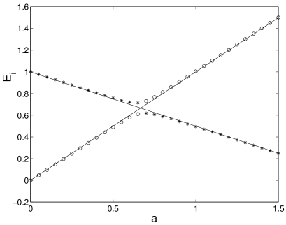
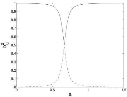
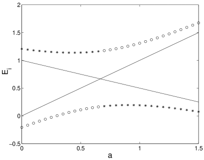
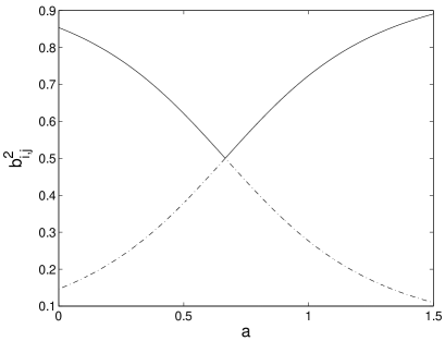
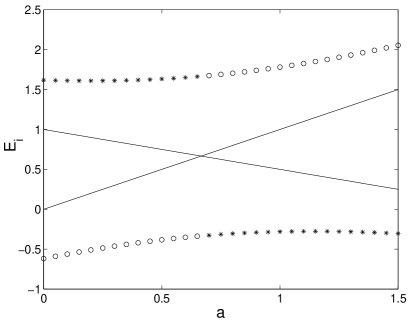
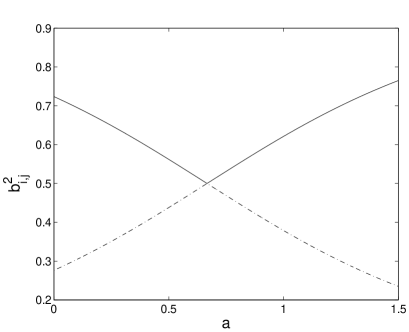
FIG. 1.: The energies $E_{i}$ (left) and mixing coefficients $b_{i,j}^{2}$ (right) for two states $i=1,2$ as a function of $a$ for $v=0.05$ (top), 0.5 (middle) and 1.0 (bottom). The circles ($i=1$) and stars ($i=2$) on the left-hand side show the energies of the two states at $v\neq 0$ and the full lines show their energies for $v=0$ (which cross at $a=a^{\rm cr}=2/3$). The full lines on the right-hand side are the coefficients $b_{i,j=i}^{2}$ while the dashed lines are the $b_{i,j\neq i}^{2}$. Note the different scales (top, middle and bottom) of the $E_{i}$ and $b_{i,j}^{2}$ axes.

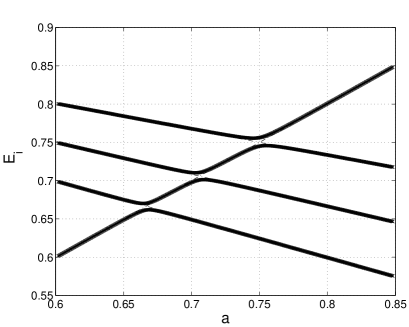
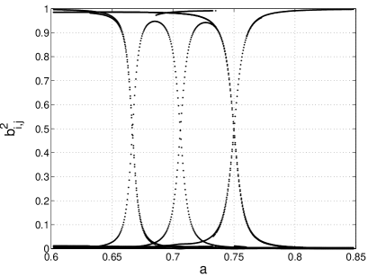
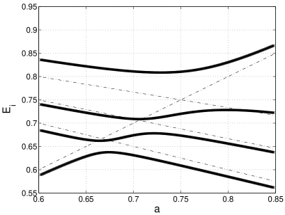
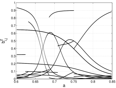
FIG. 2.: The energies $E_{i}$ (left) and mixing coefficients $b_{i,j}^{2}$ (right) for four states as a function of $a$ at $v=0.005$ (top) and 0.03 (bottom) for all coupling matrix elements. The full lines on the left-hand side show the energies of the states at $v\neq 0$ and the dash-dotted lines show their energies at $v=0$. It is $b_{i,j=i}^{2}\geq b_{i,j\neq i}^{2}$ ($\;b_{i,j=i}^{2}=b_{i,j\neq i}^{2}=0.5$ at $a_{i}^{\rm cr}$) for all $i$ at small $v$ (top right) as in figure 1. At large $v$, every state is mixed with all the other ones and an unequivocal identification of the $i$ and $j$ in the mixing coefficients $b_{i,j}^{2}$ is impossible.

REFERENCES

- [1] V. Zelevinsky, B.A. Brown, N. Frazier, and M. Horoi, Phys. Rep. 276, 85 (1996); V. Zelevinsky, Ann. Rev. Nucl. Part. Sci. 46, 237 (1996)
- [2] V.V. Flambaum, A.A. Gribakina, G.F. Gribakin and M.G. Kozlov, Phys. Rev. A 50, 267 (1994); V.V. Flambaum, G.F. Gribakin and F.M. Izrailev, Phys. Rev. E 53, 5729 (1996)
- [3] V.V. Flambaum and F.M. Izrailev, Phys. Rev. E 56, 5144 (1997) and 61, 2539 (2000)
- [4] V.K.B. Kota and R. Sahu, Phys. Lett. B 429, 1 (1998) and Phys. Rev. E 62, 3568 (2000)
- [5] C.W. Johnson, G.F. Bertsch and D.J. Dean, Phys. Rev. Lett. 80, 2749 (1998); C.W. Johnson, G.F. Bertsch, D.J. Dean and I. Talmi, Phys. Rev. C 6101, 4311 (2000)
- [6] R. Bijker, A. Frank, and S. Pittel, Phys. Rev. C 6002, 1302 (1999)
- [7] L. Kaplan and T. Papenbrock, Phys. Rev. Lett. 84, 4553 (2000)
- [8] D. Mulhall, A. Volya and V. Zelevinsky, Phys. Rev. Lett. 85, 4016
- [9] S. Drożdż and M. Wójcik, arXiv:nucl-th/0007045
- [10] J.B. French and S.S.M. Wong, Phys. Lett. B 33, 449 (1970); O. Bohigas and J. Flores, Phys. Lett. B 34, 261 (1971) and 35, 383 (1971); F.S. Chang, J.B. French and T.H. Thio, Annals of Physics 66, 137 (1971); S.S.M. Wong and J.B. French, Nucl. Phys. A 198, 188 (1972)
- [11] J. Flores, M. Horoi, M. Müller and T.H. Seligman, Phys. Rev. E 6302, 6204 (2001)
- [12] R.G. Newton, Scattering Theory of Waves and Particles, Springer-Verlag New York, 1982
- [13] E. Persson, T. Gorin and I. Rotter, Phys. Rev. E 54, 3339 (1996) and 58, 1334 (1998)
- [14] A.I. Magunov, I. Rotter and S.I. Strakhova, J.Phys.B 32, 1669 (1999) and 34, 29 (2001)
- [15] M. Müller, F.M. Dittes, W. Iskra and I. Rotter, Phys. Rev. E 52 5961 (1995)
- [16] O. Latinne, N.J. Kylstra, M. Dörr, J. Purvis, M. Terao-Dunseath, C.J. Joachain, P.G. Burke and C.J. Noble, Phys. Rev. Lett. 74, 46 (1995); N.J. Kylstra, M. Dörr, C.J. Joachain and P.G. Burke, J. Phys. B 28 L685 (1995)
- [17] J.G. Story, D.I. Duncan and T.F. Gallagher, Phys. Rev. Lett. 70, 3012 (1993); R.B. Vrijen, J.H. Hoogenraad, H.G. Muller and L.D. Noordam, Phys. Rev. Lett. 70, 3016 (1993)
- [18] E. Persson, K. Pichugin, I. Rotter and P. eba, Phys. Rev. E 58, 8001 (1998); P. eba, I. Rotter, M. Müller, E. Persson and K. Pichugin, Phys. Rev. E 61, 66 (2000); I. Rotter, E. Persson, K. Pichugin and P. eba, Phys. Rev. E 62, 450 (2000)
- [19] E. Persson, I. Rotter, H.J. Stöckmann and M. Barth, Phys. Rev. Lett. 85, 2478 (2000)
- [20] I. Rotter, Rep. Progr. Phys. 54, 635 (1991)
- [21] S. Drożdż, J. Okołowicz, M. Płoszajczak, and I. Rotter, Phys. Rev. C 62, 024313 (2000)
- [22] W. Iskra, M. Müller and I. Rotter, J. Phys. G 19, 2045 (1993) and 20, 775 (1994)