Unconditional Security of Practical Quantum Key Distribution

1 Introduction

We present a proof of unconditional security of a practical quantum key distribution protocol. It is an extension of a previous result obtained by Mayers [1, 2], which proves unconditional security provided that a perfect single photon source is used. In present days, perfect single photon sources are not available and, therefore, practical implementations use either dim laser pulses or post-selected states from parametric downconversion. Both practical signal types contain multi-photon contributions which characterise the deviation from the ideal single-photon state. This compromise threatens seriously the security of quantum key distributions when the loss rate in the quantum channel is high [3, 4, 5]. Security of such practical realisation has nevertheless been proven in [6] against restricted type of eavesdropping attacks. The salient idea used in [6] is that data associated with multiple photon signals are revealed to a possible eavesdropper, without the legitimate user’s knowledge. We show here that this model can be combined with Mayers’ proof. The resulting extension guarantees unconditional security of a realistic quantum key distribution protocol against an enemy with unlimited classical or quantum computational power.

By now, Mayers’ proof has been followed up by other proof of the security of ideal single-photon quantum key distribution [7, 8]. Security assuming some restrictions on eavesdropper’s attack can be found in [9, 10, 11]. Security of protocols in which honest participants use trusted quantum computers can be found in [12].

Unconditional security of a protocol means a security against a cheater with unlimited computational power, quantum or classical. In other words, it means that there is no condition on the cheater. It does not mean that there is no condition on the apparatus used by the honest participants. This last interpretation would be equivalent to say that we know nothing about the protocol that is actually implemented. So, each proof of unconditional security must use a different type of assumptions on these apparatus. Mayers’ original proof applies to an unrestricted eavesdropper’s attack on the quantum signals, but assumes the source used in the protocol is perfect. In particular, it assumes that the source emits single photon pulses. In this paper, we present a derivation of the proof in which the last assumption is relaxed: we still consider sources that perform perfect polarisation encoding, but each signal carries now a random number of photons in the ideal polarisation mode. The random variables giving the numbers of photons in the pulses are assumed to be identically and independently distributed, and we require that an upper-bound on the probability that a pulse contains several photons is known. As in Mayers’ original paper, there is no assumption on the quantum channel nor on the detection unit, except that, given an input quantum state of any signal, the detector’s probability of detecting a signal does not depend on the choice of the measurement basis. A more detailed discussion about assumptions in quantum cryptography together with a new approach to this problem, especially the problem of an untrusted BB84 source, can be found in [13].

This paper is divided into two parts. In the first part we define the assumptions of our proof, the protocol we refer to and the security notion. We then give the result of our proof which give the precise quantitative meaning of our security proof together. In that step the necessary parameters of the protocol leading to secure quantum key cryptography are given. We illustrate the results by giving the asymptotic formulas for the limit of long keys which show, how many secure bits the protocol will obtain for a given error rate of an experimental set-up as a function of the source parameters and the error rate. In the second part, we present the detailed proof of the statements of the first part. We have chosen to give all details of this proof to make it self contained, although it follows closely Mayers original work. The readers are invited to refer to the original paper [2] where a simpler situation was analysed, to get an insight into the main idea of the proof.

2 Security in Quantum Key Distribution

The rôle of key distribution between two distant legitimate parties, traditionally called Alice and Bob, is to generate a shared random binary string, called the private key, that is guaranteed to be known only by the legitimate parties. A non-authorised party, traditionally called Eve, should not be able to obtain any information about the private key. More precisely, for any eavesdropping strategy Eve chooses, the conditional entropy of the private key, given the data Eve acquires during the protocol, should be very close to the maximum entropy, corresponding to a uniformly and independently distributed key. One requirement for this is that the conditional probability of the private key given Eve’s data must be very close to the uniform distribution. Note that it is not sufficient to impose that the private key be independent of the data Eve acquires: a key distribution protocol that returns a specific value for the private key with high probability does not provide any privacy, even if Eve is inactive during the key distribution.

Quantum key distribution protocols do not allow Alice and Bob to share a private key in all circumstances. For example, Eve can usually block signals between the two parties. But even if the signals arrive, Alice and Bob cannot always create a secure key using them. As shown in [5], it is in principle not possible to create a secure key with the BB84 protocol (using ideal signals) once the error rate exceeds 25 %. This is true for any post-processing of the data in the sense of advantage distillation or similar ideas. It is therefore characteristic for any full protocol (including the classical post-processing of the data) that it can deliver a secure private key only as long as the parameters describing the transmission of the quantum channel (like the error rate) are within a certain parameter region.

Any protocol therefore provides a validation test that tells whether a key can be generated with unconditional privacy. A key is created only if the test is passed. Otherwise the session is abandoned. Naturally, one would like to find an entropic bound given the validation test is passed. However, it is known that such a bound is inappropriate for the protocol we consider in this paper (see for example [7]): there are simple attacks that give full knowledge about the private key, although with very small probability of success. It is therefore important to choose a good measure of privacy which nevertheless reflects our basic intuition.

We follow Mayers’ proof and define formally a key even in the cases that the validation test is not passed. For this purpose Bob formally chooses with uniform distribution a binary sequence as key whenever the test fails. We then bound Eve’s entropy on this always defined key, conditioned on her knowledge, to be arbitrarily close to the maximal value. Naturally, in that case Alice and Bob do not share a key, but this is unimportant since they are aware of it.

This choice of security notion assures that Eve’s conditional entropy is close to the maximal amount, but this situation can arise from two different scenarios: either Eve applies only gentle eavesdropping, which passes the validation tests and gives her basically no information, or she applies massive eavesdropping, which basically all the time fails the validation test, but in the unlikely event of passing the test, it might reveal substantial amount of information. Nevertheless, in both cases the key will be safe, since in the first scenario Eve has no information on the key, while in the second case, the probability of success will be, in a quantified way, extremely low.

Another important aspect of security of quantum key distribution protocols is the integrity or the faithfulness of the distributed key. We must require that whatever Eve does, it is very unlikely that Alice and Bob fail to share an identical private key while the validation test is passed. One way this situation might arise is the error correction procedure (which is a typical ingredient of a full protocol) failing to correct all errors, for example because of an unusual error distribution.

Finally, we consider families of protocols for which a parameter, quantifying the amount of a resource used in a protocol, characterises its security. Usually, the higher this security parameter’s value is, the higher is the level of security, but also the amount of a resource required by the protocol. In the protocol we consider the number of quantum signals sent by Alice as security parameter.

We now give a formal definition of security. For this we will introduce some notation. A random variable will always be denoted by a bold letter, and values taken by this random variable by the corresponding plain letter. Only discrete random variables will be considered in this paper. The probability distribution of a random variable $\boldsymbol{x}$ is denoted by ${\rm P}_{\boldsymbol{x}}$, i.e. ${\rm P}_{\boldsymbol{x}}(x)=\Pr(\boldsymbol{x}=x)$ is the probability that $\boldsymbol{x}$ takes the value $x$. The joint distribution of two random variables $\boldsymbol{x}$ and $\boldsymbol{y}$ is denoted by ${\rm P}_{\boldsymbol{xy}}$, i.e. ${\rm P}_{\boldsymbol{xy}}(x,y)=\Pr(\boldsymbol{x}=x,\boldsymbol{y}=y)$. The conditional probability of $\boldsymbol{x}$ given an event $\mathcal{E}$ with positive probability is denoted by ${\rm P}_{\boldsymbol{x}\,|\,\mathcal{E}}$, i.e. ${\rm P}_{\boldsymbol{x}\,|\,{\mathcal{E}}}(x)=\Pr(\boldsymbol{x}=x|{\mathcal{E}})$. The conditional probability of $\boldsymbol{x}$ given that $\boldsymbol{y}$ takes a value $y$ is denoted by ${\rm P}_{\boldsymbol{x}\,|\,\boldsymbol{y}=y}$ whenever ${\rm P}_{\boldsymbol{y}}(y)>0$, i.e. ${\rm P}_{\boldsymbol{x}\,|\,\boldsymbol{y}=y}(x)=\Pr(\boldsymbol{x}=x|\boldsymbol{y}=y)=\frac{{\rm P}_{\boldsymbol{xy}}(x,y)}{{\rm P}_{\boldsymbol{y}}(y)}$, whenever ${\rm P}_{\boldsymbol{y}}(y)$ is positive. Let $f$ be a function defined on the image of $\boldsymbol{x}$. When no confusion is possible, the notation $\boldsymbol{f}$ will be adopted to denote the random variable $f(\boldsymbol{x})$.

We will denote by $\boldsymbol{\vec{\kappa}}$ the random variable giving the private key generated in a key distribution session. The key is a string of $m$ bits where $m$ is a positive integer specified by the legitimate users. That is $\boldsymbol{\vec{\kappa}}$ takes value in $\{0,1\}^{m}$. We denote by valid the random variable giving the outcome of the validation test and by share the random variable telling whether Alice and Bob share an identical private key. Given an eavesdropping strategy chosen by Eve, we denote by $\boldsymbol{v}$ the random variable giving collectively all data Eve gets during this key distribution session. Henceforth, given the eavesdropping strategy adopted by Eve, $\boldsymbol{v}$ is called the view of Eve, and we will denote by ${\mathcal{Z}}$ the set of all values $\boldsymbol{v}$ may take.

We adopt the following definition of security for quantum key distribution protocols.

Definition 1

Consider a quantum key distribution protocol returning a key $\boldsymbol{\vec{\kappa}}\in\{0,1\}^{m}$ regardless of the outcome of the validation test, where the length of the key, $m$, is fixed and chosen by the user. We say that the protocol has (asymptotic) perfect security if and only if:

• the protocol is parametrised by a parameter $N$ taking value in ${\bf I\!N}$ called the security parameter, and

• there exists two functions $\epsilon_{1},\,\epsilon_{2}\,:\,{\bf I\!N}\times{\bf I\!N}\rightarrow{\bf R}^{+}$ such that $\epsilon_{1}(N,m)$ and $\epsilon_{2}(N,m)$ are vanishing exponentially as $N$ grows (i.e. there exist $\alpha>0$, $\beta>0$, $N_{min}\in{\bf I\!N}$ and a function $f:\,{\bf I\!N}\rightarrow{\bf R}^{+}$ such that $\forall N>N_{min},\,\epsilon_{1}(N,m),\,\epsilon_{2}(N,m)<e^{-\alpha N^{\beta}}f(m)$) , and

• there exists a function $N_{0}\;:\;{\bf I\!N}\rightarrow{\bf I\!N}$ such that, for any strategy adopted by Eve,

  $$\forall m,\forall N\geq N_{0}(m),$$ (1)

  (privacy) $$\quad H(\boldsymbol{\vec{\kappa}}|\boldsymbol{v})\geq m-\epsilon_{1}(N,m)$$

  (integrity) $$\quad\Pr(\neg\boldsymbol{\mbox{\bf share}}\mbox{ \rm and }\boldsymbol{\mbox{\bf valid}})\leq\epsilon_{2}(N,m)$$ (2)

  where $\boldsymbol{v}$ is Eve’s view given her strategy, and $H(\boldsymbol{\vec{\kappa}}|\boldsymbol{v})\stackrel{{\scriptstyle Def}}{{=}}-\sum_{\vec{\kappa},v\,|\,{\rm P}_{\boldsymbol{\vec{\kappa}v}}(\vec{\kappa},v)>0}{\rm P}_{\boldsymbol{\vec{\kappa}v}}(\vec{\kappa},v)\log_{2}{\rm P}_{\boldsymbol{\vec{\kappa}}\,|\,\boldsymbol{v}=v}(\vec{\kappa})$ is the Shannon entropy [14, 15, 16] of the key $\boldsymbol{\vec{\kappa}}$ given Eve’s view $\boldsymbol{v}$.

We will show that the protocol presented in the next section will be secure according to this definition. In particular, this means, that the protocol creates a key of length $m$ out of $N$ signals. Then, by choosing $N$ large enough for fixed values of $m$, we can always assure that Eve’s conditional entropy is arbitrarily close to the maximum amount (privacy). Additionally, with a probability arbitrarily close to unity, Alice and Bob share the key given that the validation test is passed (integrity).

3 The protocol

In this section, the quantum key protocol considered in this paper is described. It is an adaptation of the BB84 [17] protocol which takes into account the usage of an imperfect photon source. Note that the usage of imperfect source has been discussed as early as the first experimental implementation of BB84 [18] in the framework of restricted types of eavesdropping attacks. We first make precise which assumptions on the quantum channel we adopt in this paper. Then we give a formal description of the protocol.

3.1 Required technology

In the original proof [2], Mayers considered a practical realisation of quantum key distribution prone to noise and signal loss. However, the legitimate parties were assumed to be using a perfect single photon source – a source that emits exactly one photon in the chosen polarisation state. No restriction was imposed on the photo-detection unit used in the protocol, except that given an incoming signal, the probability of detection was required to be independent of the basis used to measure the signal. It was argued in [2] that Eve can take advantage of a detection unit in which the probability of detection depends on the basis chosen for the measurement, and we will adopt in this paper the same restriction regarding the detection unit.

The new feature in this paper is that we allow the use of imperfect source of photons in the following sense: given a polarisation state specified by the user, the source emits photons exactly in the specified polarisation state, but in a mixture of Fock states. That is, the source emits $n$ photons in the given polarisation state with probability $p_{n}$, where $n\in{\bf I\!N}$ and $p_{0},p_{1},p_{2},\ldots$ is a probability distribution. The user does not have to know how many photons were actually emitted. The only restriction we impose is that an upper bound $M_{max}$ on the number of emitted signals containing several photons is known within a confidence limit given by the (small) probability $Pr(M>M_{max})$. We restrict ourselves to provide this bound for signals with identically and independently distributed multi-photon probability $p_{M}$. In that case we can choose $M_{max}=(p_{M}+\tau_{M})N$ and obtain $Pr(M>M_{max})<\exp(-\tau_{M}^{2}N)$, as explained below. Other methods for providing $M_{max}$ and $Pr(M>M_{max})$ can be used, where the corresponding terms replace the here derived and easily identifiable expressions in the subsequent results.

The authors believe this relaxation of requirement has practical importance, since single photon sources are not yet available, due to technological limitations. Furthermore, it has been pointed out [5] that in most experimental implementations of quantum key distribution, the quantum signals transmitted by the legitimate parties can be described as mixtures of Fock states.

As an example, consider a practical source emitting a coherent state of light in a given polarisation:

$$\big{|}\,\alpha\big{\rangle}=e^{-\frac{|\alpha|^{2}}{2}}\sum_{j=0}^{\infty}\frac{\alpha^{j}}{\sqrt{j!}}\big{|}\,j\big{\rangle}$$ (3)

where $\big{|}\,j\big{\rangle}$, $j\in{\bf I\!N}$ is the number state – or Fock state – describing a state of $j$ photons in the considered polarisation (Therefore, for $\alpha\neq 0$, a coherent state has an indefinite number of photons). If we write $\alpha=|\alpha|e^{i\phi}$, $|\alpha|$ and $\phi$ are called amplitude and phase of the coherent pulse, respectively.

In general, the phase of a pulse is completely unknown, or can be rendered random thanks to a phase randomisation technique. Since the phase is then uniformly distributed, a pulse state in a given polarisation is described by the density matrix:

$$\rho_{\mbox{source}} = \frac{1}{2\pi}\int_{0}^{2\pi}\big{|}\,|\alpha|e^{i\phi}\big{\rangle}\big{\langle}|\alpha|e^{i\phi}\,\big{|}d\phi$$ (4)

$$= \frac{1}{2\pi}\int_{0}^{2\pi}e^{-|\alpha|^{2}}\sum_{j,j^{\prime}=0}^{\infty}\frac{|\alpha|^{j+j^{\prime}}}{\sqrt{j!j^{\prime}!}}e^{i\phi(j-j^{\prime})}\big{|}\,j\big{\rangle}\big{\langle}j^{\prime}\,\big{|}d\phi$$ (5)

$$= \sum_{j=0}^{\infty}e^{-|\alpha|^{2}}\frac{|\alpha|^{2j}}{j!}\big{|}\,j\big{\rangle}\big{\langle}j\,\big{|}$$ (6)

Therefore, the signals emitted by a coherent source of light becomes a classical mixture of Fock states due to the lack of a phase reference. Another example of practical source is a source emitting thermal states of light. Such states are already mixtures of Fock states. The above de-phasing argument applies in general for any signal state. Further studies of source characterisation can be found in [19].

We summarise the assumptions on the quantum setup adopted throughout this paper:

• The legitimate parties use a source of photons that sends a mixture of Fock states $\rho=\sum_{n=0}^{\infty}p_{n}\big{|}\,n\big{\rangle}\big{\langle}n\,\big{|}$ in the polarisation state exactly as specified by the user. The numbers of photons in the pulses emitted by the source are assumed to be identically and independently distributed. The upper bound $M_{max}$ on the emitted number of multi-photon signals during the protocol is known by the legitimate parties to hold except with a negligible probability $Pr(M>M_{max})$.

• The legitimate parties use a photo-detection unit such that for any given signal, the probability of detection is independent of the choice of the measurement basis.

• The signals and Alice’s and Bob’s polarization bases are chosen truly at random.

• Eve cannot intrude Alice’s or Bob’s apparatus by utilizing the quantum channel. She is restricted to interaction with the signals as they pass along the quantum channel.

3.2 The protocol

The quantum key distribution protocol under consideration based on Bennett and Brassard’s BB84 [17] is defined. It comprises three stages: agreement on parameters of the protocol and security constants, the transmission of quantum signals, and the execution of a classical protocol together with the validation test.

Pre-agreement

1. Alice and Bob specify:

   • $m$, the length (in bits) of the private key to be generated.

   • $N$, the number of quantum signals to be sent by Alice. This integer is the security parameter of the protocol.

   • $\delta$, the maximum threshold value for the error rate for the validation test.

   • $r_{min}$, the minimum threshold value for Bob’s detection rate ($1>r_{min}>M_{max}/N$).

   • $p_{R}$, the proportion of the shared bits that must be publicly announced for the validation test ($0<p_{R}\leq 1/2$).

   • $\tau_{ec}$, $\tau_{f}$, $\tau_{M}$, $\hat{\tau}$, and $\tau_{p}$ the security constants of the protocol. They are small strictly positive real numbers chosen so that $\delta+\tau_{ec}<1$, $\delta+\tau_{f}<1$, $r_{min}>M_{max}/N$, $\hat{\tau}<\frac{1-p_{R}}{2}$, $\tau_{p}<1$.

Quantum Transmission

1. Alice and Bob initialise the counter of the signals as $i=0$ and Bob initialises the set of detected signals as $\mathcal{D}=\{\}$. Then until the pre-agreed number of signals have been sent ($i=N$), the following is repeated

   1. Alice and Bob increment $i$ by one.

   2. Alice picks randomly with uniform distribution a basis $a_{i}\in\{+,\times\}$ and a bit value $g_{i}\in\{0,1\}$.

   3. Alice makes her source emit a pulse of photons in the state $\left|\,\Psi(g_{i},a_{i})\right\rangle$ where $\left|\,\Psi(0,+)\right\rangle$, $\left|\,\Psi(1,+)\right\rangle$, $\left|\,\Psi(0,\times)\right\rangle$ and $\left|\,\Psi(1,\times)\right\rangle$ correspond to single photon states of polarisation angles 0, $\pi/2$, $\pi/4$ and $-\pi/4$, respectively. We recall that $\{\big{|}\,\Psi(0,+)\big{\rangle},\big{|}\,\Psi(1,+)\big{\rangle}\}$ forms an orthonormal basis of ${\mathcal{H}}_{\textrm{\scriptsize{photon}}}$, the Hilbert space for single photon polarisation states, and $\big{|}\,\Psi(0,\times)\big{\rangle}=\frac{\big{|}\,\Psi(0,+)\big{\rangle}+\big{|}\,\Psi(1,+)\big{\rangle}}{\sqrt{2}}$, $\big{|}\,\Psi(1,\times)\big{\rangle}=\frac{\big{|}\,\Psi(0,+)\big{\rangle}-\big{|}\,\Psi(1,+)\big{\rangle}}{\sqrt{2}}$.

   4. Bob measures Alice’s pulse in the basis $b_{i}$ where $b_{i}\in\{+,\times\}$ is chosen randomly at each time. If at least one photon is detected, the index $i$ is added to the set $\mathcal{D}$ of detected signals’ indexes, and the outcome of the measurement is recorded as $h_{i}\in\{0,1\}$ (if the detection unit finds photons in both modes $h_{i}=0,1$, the value for $h_{i}$ is chosen randomly in $\{0,1\}$ by Bob). If no photon is detected at all, $h_{i}$ is assigned the value $\perp$.

Note that the random choice of basis in step (d) might be provided by a beamsplitter (or a coupler) followed by two measurement setups, each measuring the photons in the basis $+$ and $\times$ respectively. It might also be given by an external random number generator acting on a polarisation rotator.

Classical part

We denote by $n$ the number of signals detected by Bob, i.e. $n=|\mathcal{D}|$, and by $\vec{a}=(a_{1},\ldots,a_{N})\in\{+,\times\}^{N}$, $\vec{b}=(b_{1},\ldots,\vec{b}_{N})\in\{+,\times\}^{N}$, $\vec{g}=(g_{1},\ldots,g_{N})\in\{0,1\}^{N}$ and $\vec{h}=(h_{1},\ldots,h_{N})\in\{0,1,\perp\}^{N}$ the outcome of the quantum transmission (Step 2). Restrictions of these vectors onto some specified subset $X\subset\{1,\dots,N\}$ will be denoted by $\vec{a}(X),\vec{b}(X),\vec{g}(X),\vec{h}(X)$.

1. Bob announces the set of detected signals by $\mathcal{D}$ to Alice.

2. Bob picks up randomly a subset of signals which will be revealed for the validation test $R\subset\{1,\ldots,N\}$ , where each position $i\in\{1,\ldots,N\}$ is put in $R$ with probability $p_{R}$.

3. Bob announces the revealed set $R$ and the measurement basis of all signals $\vec{b}$ to Alice.

4. Bob announces the bit values of the test set $\vec{h}(\mathcal{D}\cap R)$ to Alice.

5. Alice computes the set of corresponding signals $\Omega=\{i\in\mathcal{D}\,:\,a_{i}=b_{i}\}$, the set of corresponding test signals $T=\Omega\cap R$ and the set of untested corresponding signals $E=\Omega\cap\overline{R}$. We denote $|E|$ by $l$.

6. Alice announces the polarisation basis of all of her signals $\vec{a}$, thus announces implicitly $\Omega$ and $E$ as well. The bitstreams $\vec{g}(E)$ and $\vec{h}(E)$ are usually called sifted keys.

7. Alice chooses a linear error correcting code [14, 15] capable of correcting $\lceil(\delta+\tau_{ec})(1-p_{R})|\Omega|\rceil$ errors in $E$. Its parity check matrix, $F$, is a $r\times l$ binary matrix, where $r$ is the number of redundant bits required to correct $\lceil(\delta+\tau_{ec})(1-p_{R})|\Omega|\rceil$ errors in $l$ bits using the linear error correcting code. Alice announces the syndrome $\vec{s}=F\vec{g}(E)\pmod{2}$ to Bob.

8. Receiving the parity check matrix $F$ and the syndrome $\vec{s}$, Bob runs the error correction on his sifted key $\vec{h}(E)$ and obtains $\vec{h}^{\prime}(E)$. If there are less than $\lceil(\delta+\tau_{ec})(1-p_{R})|\Omega|\rceil$ errors in $E$, Bob corrects successfully all the errors and obtains $\vec{g}(E)$, i.e. $\vec{h}^{\prime}(E)=\vec{g}(E)$.

9. Alice picks up randomly with uniform distribution a $m\times l$ binary matrix $K$ to which we will refer as the privacy amplification matrix. Alice announces $K$ publicly.

10. Receiving the privacy amplification matrix $K$, Bob computes $\vec{\kappa}^{\prime}=K\vec{h}^{\prime}(E)\pmod{2}$.

Validation test

Alice runs the validation test.

1. Alice tests whether the following conditions are all satisfied:

   • Bob’s detection rate is greater than $r_{min}$, i.e.

     $$n>r_{min}N.$$ (7)

   • The size of $\mathcal{D}$ complies to the following inequalities:

     $$\frac{\widehat{l}_{min}}{2} \geq (\delta+\tau_{f})(1-p_{R})n,$$ (8)

     $$m+r \leq \widehat{l}_{min}\left[1-H_{1}\left[\frac{2(\delta+\tau_{f})\frac{1-p_{R}}{2}n}{\widehat{l}_{min}}\right]-\tau_{p}\right],$$ (9)

     where

     $$\widehat{l}_{min}=\left(\frac{1-p_{R}}{2}-\hat{\tau}\right)(n-M_{max})$$ (10)

     is a probabilistic lower bound on the number of signals on the set $E$ which is due to single photon signals.

   • The number of errors in the tested set $T$ is lower than the maximally allowed value. More precisely,

     $$\left|\{i\in T\,:\,g_{i}\neq h_{i}\}\right|<d,$$ (11)

     where $d=\delta|\Omega|p_{R}$.

   The validation test is passed if and only if all the conditions above are satisfied. The private key is the bitstream obtained by Alice as follows:

2. Alice computes the private key, defined as:

   • $\vec{\kappa}=K\vec{g}(E)\pmod{2}$ if the validation test is passed,

   • a $m$-bit string $\vec{\kappa}$ chosen randomly with uniform distribution each time the validation test is not passed.

This protocol defines a key regardless whether the validation test is passed. The choice of the security constants used in the protocol is clarified in the following section.

Note:

The matrix $K$ can be prepared in advance, and Eve could know its form before the transmission of the quantum signal. More precisely, Alice and Bob could pre-agree on some set of matrices $K$ for various values of $m$, and $l$. It is the special property 4 of $F$ and $K$ which is required here, and which will be introduced and explained in the section 5.3. This property is satisfied automatically if we choose $K$ as random binary matrix, as specified in the protocol, and the constraint of Eq. 9 is satisfied. Our security proof can therefore immediately adapted to other choices of $F$ and $K$ together with their respective constraints replacing Eq 9 to satisfy the underlying required property 4 of section 5.3.

4 Security of the protocol

In this section we present the security statement for the protocol described in 3.2. If follows the structure of Def. 1. The proof of the security statement is given in the remainder of the paper.

Theorem 1

The expected conditional Shannon entropy of the key $\boldsymbol{\vec{\kappa}}$ returned by the protocol described in Section 3.2 given Eve’s view $\boldsymbol{v}$ is lower bounded, for any $N>0$, by

$$H(\boldsymbol{\vec{\kappa}}|\boldsymbol{v})\geq m-\epsilon_{1}(N,m)$$ (12)

where the difference $\epsilon_{1}(N,m)$ between the bound and the maximal value $m$ is given by

$$\epsilon_{1}(N,m) = 2\left(m+\frac{1}{\ln 2}\right)h(\delta,\tau_{f},p_{R},n)+2\sqrt{2\left(m+\frac{1}{\ln 2}\right)mh(\delta,\tau_{f},p_{R},n)}+$$ (13)

$$+ m\Big{(}e^{-2\tau_{M}^{2}N}+e^{-2\hat{\tau}^{2}(r_{min}N-M_{max})}+2^{-\tau_{p}\left(\frac{1-p_{R}}{2}-\hat{\tau}\right)(r_{min}N-M_{max})}+$$

$$+ \sqrt{g(\delta,\tau_{f},p_{R},n)}\Big{)}.$$

where

$$g(\delta,\tau_{f},p_{R},n) = \exp\left[-\frac{1}{2\delta+\tau_{f}}\tau_{f}^{2}\frac{p_{R}^{2}}{4}r_{min}N+2\left(\frac{\tau_{f}}{2\delta+\tau_{f}}\right)^{2}\right],$$ (14)

$$h(\delta,\tau_{f},p_{R},n) = 2\sqrt{\sqrt{g(\delta,\tau_{f},p_{R},n)}}+\sqrt{g(\delta,\tau_{f},p_{R},n)}.$$ (15)

Besides, the conditional probability that Alice and Bob share an identical private key given that the validation test is passed is lower bounded for any $N>0$ by:

$$\Pr(\neg\mbox{\bf share}\mbox{ \rm and }\mbox{\bf valid})\leq\epsilon_{2}(N,m),$$ (16)

where

$$\epsilon_{2}(N,m)=\min_{\tau_{\Omega}\in(0,1/2)}\left[e^{-\frac{1}{2\delta+\tau_{ec}}\tau_{ec}^{2}p_{R}^{2}(\frac{1}{2}-\tau_{\Omega})r_{min}N+2\left(\frac{\tau_{ec}}{2\delta+\tau_{ec}}\right)^{2}}+e^{-2\tau_{\Omega}^{2}r_{min}N}\right]\;.$$ (17)

The functions $\epsilon_{1}(N,m)$ and $\epsilon_{2}(N,m)$ decrease exponentially with $N$, as required by the definition of security (Definition 1).

The parameters, the number of emitted signals $N$ out of which the key of length $m$ is created, are chosen in accordance with the performance of the set-up used for preparation, transmission and detection of the quantum signals in view of Equation 9. As the number of these transmissions goes to infinity, we can neglect statistical fluctuations of the signal properties and describe the ratio between detected signals and sent signals by a detection rate $p_{D}=n/N$ and $r_{min}=n/N$. All security constants $\tau_{ec}$, $\tau_{f}$, $\tau_{p}$, $\tilde{\tau}$ and $\tau_{M}$ can be chosen to be arbitrarily small, and the asymptotic key generation rate out of one bit of the sifted key reads is given as the length of the sifted key over that of the final key in terms of the observed error rate $\delta$ as

$$\frac{m}{l}=\left(1-\frac{p_{M}}{p_{D}}\right)\left[1-H_{1}\left(\frac{2\delta}{1-\frac{p_{M}}{p_{D}}}\right)\right]-H_{1}(\delta)\;.$$ (18)

Here we used we used asymptotic equalities for the sifted key length $l\simeq\frac{1-p_{R}}{2}n$ and $\lceil(\delta+\tau_{ec})(1-p_{R})|\Omega|\rceil\simeq\lceil\delta l\rceil$. Furthermore, we made use of the Shannon limit [14] $r(\lceil\delta l\rceil,l)\simeq lH_{1}(\delta)$.

The overall rate of secure key bits per sent signal $m/N$ can be calculated directly by multiplying Eq. (18) with the asymptotic formula

$$\frac{l}{N}\simeq\frac{1-p_{R}}{2}p_{D}\;.$$ (19)

The ratio $G$ between key length and received signals $m/n$ can be obtained by multiplication with $l/n\simeq(1-p_{R})/2$. Moreover, in the limit of arbitrary long keys we can use the limit $p_{R}\to 0$ since even testing a ’small’ fraction of the long key will have statistical significance sufficient for our purpose. Examples of the resulting values of $G$ as a function of distance are shown in Figure 1 for various wavelength.

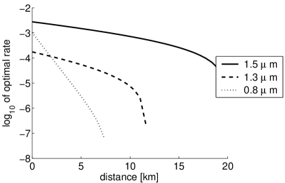
Figure 1: Asymptotic gain rates using a simulation with the help of experimental parameters. The parameters are drawn from Bourennane et al. [20] for $1.5\mu m$, Marand and Townsend [21] for $1.3\mu m$ and Townsend [22] for $0.8\mu m$.

To put our results into context, we relate our results in Fig. 2 to those obtained for the limited security level of security against individual attacks. Note that the difference between the two results is not substantial. More importantly, the difference might be due to the proof technique used in our result. Our results should therefore not be interpreted as to claim that coherent attacks give more information to Eve than individual attacks do.

Figure 2: We use the parameters of Bourennane et al. [20] for $1.5\mu m$ to show the secure gain rate per time slot using our results (’coherent’). For comparison, the corresponding results for security against individual attack [6] are given. The rate is bounded due to the Poissonian photon number distribution of the source and the loss in the quantum channel (’rate bound’) as shown in [6]. The combination of the source statistics, the loss and detector dark counts, there is a fundamental bound on the distance over which secure QKD could be proven with more advances proofs than ours, as shown in Brassard et al. [5]

Furthermore, we lay out the relevant bounds on improved security proofs. The rate is bounded due to the photon number statistics of the source, resulting in

$$G_{bound}=\frac{1}{2}\left(p_{D}-p_{M}\right)$$ (20)

as shown in [6]. We recover this bound by setting $\delta=0$ in our asymptotic bound.

The distance, over which secure communication is possible, is bounded by the detector noise. As shown in Brassard et al. [5], the minimal transmission efficiency $F_{WCP}$ in the situation of Poissonian photon number distribution of the source is given by

$$F_{WCP}\approx 2\frac{\sqrt{d_{B}}}{\eta_{B}}$$ (21)

where $d_{B}$ is the dark count probability of the detector per signal slot and $\eta_{B}$ is the single photon detection efficiency of the detector. The corresponding distance (given the parameters of the experiment) is shown in Fig. 2.

We have therefore a clear picture of the rates and distances which are shown to be secure by our proof (the area below the curve ’coherent’ in Fig. 2), those that are shown to be insecure [5, 6] (the area outside of the two bound curves). Note that the area between the ’coherent’ line and the two bounds is the area of the unknown. Future classical protocols taking on the error correction and privacy amplification tasks from our protocol in a different way (but leaving the quantum transmission and measurement untouched) and/or improved security proofs can proclaim more of this area ’secure’.

5 Proof of the main result

The structure of the proof follows. In the first section, an important feature of the distribution of errors during the quantum transmission is presented. As an immediate consequence we can proof the integrity of the protocol, meaning that when the validation test is passed, Bob shares the private key with Alice with high probability. The second section deals with the multi-photon signals’ issue. It gives an upper bound on the number of bits a spy can get by an attack called photon number splitting attack. In the third section, we explore the method of privacy amplification implemented by binary matrices and taking into account linear error correction tools. It turns out that the privacy of the protocol is equivalent to the “privacy” in a modified protocol . This equivalence is proved in section 5.4, and the corresponding mathematical model is provided in section 5.5. Finally, the proof of privacy of the modified protocol is given.

There are several points where our proof deviates from that of Mayers [2]. Most notably this difference can be seen in 5.3 where the deviation between the proofs shows up quantitatively . However, changes in the protocol (in our protocol the number of transmitted signals is fixed which are not necessarily all detected, and not the number of detected signals, as in [1]) make it necessary to check in detail that the basic proof idea of Mayers carries through.

5.1 On the distribution of errors and the proof of integrity

We start with a property regarding the distribution of errors which is based solely on basic probability theory. It allows to make statements on the key derived from the set $E$ based on the counting of errors in the set $T$. As an immediate application this property allows us to proof the integrity of the QKD protocol. Note, that in a practical run of quantum key distribution, we could omit this estimation, since we can learn the exact number of errors in $E$ during the later stage of error correction. However, the kind of estimation presented here serves a second purpose, which is used later on in our proof. This purpose is to make a statement about the eavesdropping strategy and its expected error rate from the observed error rate. Let us explain this by an example: If Eve implements an intercept/resend attack where she measures Alice’s bit in a randomly chosen signal basis and she resends a state to Bob corresponding to her measurement result, then she might be lucky an choose always the correct signal basis. In that (unlikely) event, she would cause no errors while obtaining full information on the key. Indirectly, the property below quantifies the idea that the observed numbers of errors will belong to a typical run of the protocol.

Property 1

Let ${\mathcal{S}}$ be a set of finite size, $s$. Let $C$ be a randomly chosen subset of ${\mathcal{S}}$. The random variable giving the choice of $C$ is denoted by $\boldsymbol{C}$. Let $A$ and $B$ be two subsets of ${\mathcal{S}}$ chosen randomly as follows:

1. Each element in ${\mathcal{S}}$ is put (exclusively) in $A$ or $B$ or neither of these sets with respective probabilities $p_{A}$, $p_{B}$ and $1-(p_{A}+p_{B})$. That is, the random variables giving the set to which the indexes in ${\mathcal{S}}$ belong to are independently and identically distributed.

2. Furthermore, the random variables giving the set to which indexes in ${\mathcal{S}}$ belong to are independent of the random variable $\boldsymbol{C}$.

We denote by $\boldsymbol{A}$, $\boldsymbol{B}$ the random variables giving the set $A$ and $B$, respectively. Then for any positive real numbers $\delta$, $\epsilon$ such that $0<\delta<\delta+\epsilon<1$,

$$\Pr(|\boldsymbol{A}\cap\boldsymbol{C}|<\delta sp_{A}\mbox{ \rm and }|\boldsymbol{B}\cap\boldsymbol{C}|\geq(\delta+\epsilon)sp_{B})\leq f(\delta,\epsilon,p_{A},p_{B},s)$$ (22)

where

$$f(\delta,\epsilon,p_{A},p_{B},s)=\exp\left[-\frac{1}{2\delta+\epsilon}\epsilon^{2}(\min\{p_{A},p_{B}\})^{2}s+2\left(\frac{\epsilon}{2\delta+\epsilon}\right)^{2}\right].$$ (23)

Proof For any subset $C$ of ${\mathcal{S}}$, given $\boldsymbol{C}=C$, each element of $C$ is either in $\boldsymbol{A}$ or in $\boldsymbol{B}$ with respective probabilities $p_{A}$ and $p_{B}$.

Now $c=|C|$ is either smaller than $\lfloor(\delta+\frac{\epsilon}{2})s\rfloor$ or bigger than $\lceil(\delta+\frac{\epsilon}{2})s\rceil$.

• If $c\leq\lfloor(\delta+\frac{\epsilon}{2})s\rfloor$, let $C^{\prime}=C\cup D$ where $D$ is some subset of ${\mathcal{S}}\setminus C$ such that $|C^{\prime}|=c^{\prime}=\lfloor(\delta+\frac{\epsilon}{2})s\rfloor$. Then $C\subset C^{\prime}$, and

  $$\Pr(|\boldsymbol{B}\cap\boldsymbol{C}|\geq(\delta+\epsilon)sp_{B}|\boldsymbol{C}=C)\leq\Pr(|\boldsymbol{B}\cap\boldsymbol{C}|\geq(\delta+\epsilon)sp_{B}|\boldsymbol{C}=C^{\prime}).$$ (24)

  Furthermore,

  $$(\delta+\epsilon)sp_{B}=\frac{\delta+\epsilon}{\delta+\frac{\epsilon}{2}}p_{B}(\delta+\frac{\epsilon}{2})s\geq(1+\frac{\epsilon}{2\delta+\epsilon})p_{B}c^{\prime},$$ (25)

  and using the Property 16 from the Appendix for the set $B$ and the set $C^{\prime}$,

  $$\Pr(|\boldsymbol{B}\cap\boldsymbol{C}|\geq(\delta+\epsilon)sp_{B}|\boldsymbol{C}=C^{\prime}) \leq \Pr(|\boldsymbol{B}\cap\boldsymbol{C}|\geq(1+\frac{\epsilon}{2\delta+\epsilon})p_{B}c^{\prime}|\boldsymbol{C}=C^{\prime})$$ (26)

  $$\leq \exp\left[-2\left(\frac{\epsilon p_{B}}{2\delta+\epsilon}\right)^{2}c^{\prime}\right]$$ (27)

  $$\leq f(\delta,\epsilon,p_{A},p_{B},s),$$ (28)

  since $(\min\{p_{A},p_{B}\})^{2}\leq p_{B}^{2}$ and $c^{\prime}\geq\left(\delta+\frac{\epsilon}{2}\right)s-1$. Of course this implies that

  $$\Pr(|\boldsymbol{A}\cap\boldsymbol{C}|<\delta sp_{A}\mbox{ \rm and }|\boldsymbol{B}\cap\boldsymbol{C}|\geq(\delta+\epsilon)s|\boldsymbol{C}=C)\leq f(\delta,\epsilon,p_{A},p_{B},s).$$ (29)

• If $c\geq\lceil(\delta+\frac{\epsilon}{2})s\rceil$, then

  $$\delta sp_{A}=\frac{\delta}{\delta+\frac{\epsilon}{2}}p_{A}(\delta+\frac{\epsilon}{2})s\leq\left(1-\frac{\epsilon}{2\delta+\epsilon}\right)p_{A}c$$ (30)

  and using the Property 16 for the set $A$ and the set $C$,

  $$\Pr(|\boldsymbol{A}\cap\boldsymbol{C}|<\delta sp_{A}|\boldsymbol{C}=C) \leq \Pr(|\boldsymbol{A}\cap\boldsymbol{C}|<\left(1-\frac{\epsilon}{2\delta+\epsilon}\right)p_{A}c|\boldsymbol{C}=C)$$ (31)

  $$\leq \exp\left[-2c\left(\frac{p_{A}\epsilon}{2\delta+\epsilon}\right)^{2}\right]$$ (32)

  $$\leq f(\delta,\epsilon,p_{A},p_{B},s),$$ (33)

  since $(\min\{p_{A},p_{B}\})^{2}\leq p_{A}^{2}\leq 1$ and $c\geq\left(\delta+\frac{\epsilon}{2}\right)s>\left(\delta+\frac{\epsilon}{2}\right)s-1$. Again, this implies that

  $$\Pr(|\boldsymbol{A}\cap\boldsymbol{C}|<\delta sp_{A}\mbox{ \rm and }|\boldsymbol{B}\cap\boldsymbol{C}|\geq(\delta+\epsilon)s|\boldsymbol{C}=C)\leq f(\delta,\epsilon,p_{A},p_{B},s).$$ (34)

We conclude that for any $C$,

$$\Pr(|\boldsymbol{A}\cap\boldsymbol{C}|<\delta sp_{A}\mbox{ \rm and }|\boldsymbol{B}\cap\boldsymbol{C}|\geq(\delta+\epsilon)s|\boldsymbol{C}=C)\leq f(\delta,\epsilon,p_{A},p_{B},s).$$ (35)

Thus

$$\Pr(|\boldsymbol{A}\cap\boldsymbol{C}|<\delta sp_{A}\mbox{ \rm and }|\boldsymbol{B}\cap\boldsymbol{C}|\geq(\delta+\epsilon)sp_{B})$$ (36)

$$= \sum_{C}{\rm P}_{\boldsymbol{C}}(C)\Pr(|\boldsymbol{A}\cap\boldsymbol{C}|<\delta sp_{A}\mbox{ \rm and }|\boldsymbol{B}\cap\boldsymbol{C}|\geq(\delta+\epsilon)sp_{B}|\boldsymbol{C}=C)$$

$$\leq f(\delta,\epsilon,p_{A},p_{B},s),$$ (37)

which concludes the proof.$\Box$

An immediate consequence of property 1 is that the error rate in the sifted key is not significantly higher than the error rate observed by Alice and Bob during the validation test. This implies the integrity of the protocol, as defined in Def. 1, or more formally:

Property 2

The joint probability that Alice and Bob fail to share an identical key and that the validation test is passed is lower bounded by:

$$\Pr(\neg\boldsymbol{\mbox{\bf share}}\mbox{ \rm and }\boldsymbol{\mbox{\bf valid}})\leq\epsilon_{2}(N,m)$$ (38)

where

$$\epsilon_{2}(N,m)=\min_{\tau_{\Omega}\in(0,1/2)}\left[e^{-\frac{1}{2\delta+\tau_{ec}}\tau_{ec}^{2}p_{R}^{2}(\frac{1}{2}-\tau_{\Omega})r_{min}N+2\left(\frac{\tau_{ec}}{2\delta+\tau_{ec}}\right)^{2}}+e^{-2\tau_{\Omega}^{2}r_{min}N}\right].$$ (39)

Proof We have seen that Alice and Bob run an error-correcting scheme capable of correcting $\lceil(\delta+\tau_{ec})(1-p_{R})|\Omega|\rceil$ errors in $E$. Thus Bob shares exactly the same key after the error correction step if there are less than $(\delta+\tau_{ec})(1-p_{R})|\Omega|$ errors in $E$. Given that $\boldsymbol{\Omega}=\Omega$ where $\Omega\subset\{1,\ldots,N\}$, the probability that the validation test passes while there are more than $(\delta+\tau_{ec})(1-p_{R})|\Omega|$ errors in $E$ is bounded by:

$$\Pr(\boldsymbol{{\mathcal{P}}}(\boldsymbol{T},\delta|\Omega|p_{R})\wedge\neg\boldsymbol{{\mathcal{P}}}(\boldsymbol{E},(\delta+\tau_{ec})|\Omega|(1-p_{R})))$$

$$= \Pr(|\boldsymbol{T}\cap\boldsymbol{C}|<\delta|\Omega|p_{R}\mbox{ \rm and }|\boldsymbol{E}\cap\boldsymbol{C}|\geq(\delta+\tau_{ec})|\Omega|(1-p_{R}))$$

$$\leq f(\delta,\tau_{ec},p_{R},1-p_{R},|\Omega|)$$

$$\leq \exp\left[-\frac{1}{2\delta+\tau_{ec}}\tau_{ec}^{2}p_{R}^{2}|\Omega|+2\left(\frac{\tau_{ec}}{2\delta+\tau_{ec}}\right)^{2}\right].$$ (41)

using the above property for ${\mathcal{S}}=\Omega$ and where $\boldsymbol{C}$ is the random variable giving the set of discrepancies between Alice’s bits $\vec{g}(\Omega)$ and Bob’s bits $\vec{h}(\Omega)$ on $\Omega$. Indeed, $\boldsymbol{R}$ is independent of $\boldsymbol{C}$, and consequently the random variables giving the set ($E$ or $T$) to which the indexes in $\Omega$ belong to are independently and identically distributed ($\Pr(i\in E|i\in\Omega)=(1-p_{R})$ and $\Pr(i\in T|i\in\Omega)=p_{R}$), and independent of $\boldsymbol{C}$. The above implies that the probability that the error correction fails to reconcile Alice’s and Bob’s sifted keys while the validation test is passed is upper-bounded by an exponentially decreasing function of $|\Omega|$. Now, each index in $\mathcal{D}$ has probability $1/2$ to be put in the set $\boldsymbol{\Omega}$. Let $\tau_{\Omega}$ be a constant obeying $0<\tau_{\Omega}<1/2$. Suppose we are given that $\boldsymbol{n}=n$ for some positive integer $n$. Using Property 16 in the Appendix, the probability that there are less than $(\frac{1}{2}-\tau_{\Omega})n$ is bounded by:

$$\Pr(|\boldsymbol{\Omega}|\leq(\frac{1}{2}-\tau_{\Omega})n\,|\,\boldsymbol{n}=n)\leq e^{-2\tau_{\Omega}^{2}n}.$$ (42)

Therefore,

$$\Pr(\neg\boldsymbol{\mbox{\bf share}}\wedge\boldsymbol{\mbox{\bf valid}})$$

$$\leq \Pr\left(\boldsymbol{{\mathcal{P}}}(\boldsymbol{T},\delta|\boldsymbol{\Omega}|p_{R})\wedge\neg\boldsymbol{{\mathcal{P}}}(\boldsymbol{E},(\delta+\tau_{ec})|\boldsymbol{\Omega}|(1-p_{R}))\,\Big{|}\,\boldsymbol{n}>r_{min}N\right)$$

$$\leq \Pr\left(\boldsymbol{{\mathcal{P}}}(\boldsymbol{T},\delta|\boldsymbol{\Omega}|p_{R})\wedge\neg\boldsymbol{{\mathcal{P}}}(\boldsymbol{E},(\delta+\tau_{ec})|\boldsymbol{\Omega}|(1-p_{R}))\,\Big{|}\,|\boldsymbol{\Omega}|\geq(\frac{1}{2}-\tau_{\Omega})\boldsymbol{n}\;,\;\boldsymbol{n}>r_{min}N\right)+$$

$$+ \Pr\left(|\boldsymbol{\Omega}|\leq(\frac{1}{2}-\tau_{\Omega})\boldsymbol{n}\,\Big{|}\,\boldsymbol{n}>r_{min}N\right)$$

$$\leq e^{-\frac{1}{2\delta+\tau_{ec}}\tau_{ec}^{2}p_{R}^{2}(\frac{1}{2}-\tau_{\Omega})r_{min}N+2\left(\frac{\tau_{ec}}{2\delta+\tau_{ec}}\right)^{2}}+e^{-2\tau_{\Omega}^{2}r_{min}N},$$ (44)

since $\boldsymbol{n}>r_{min}N$ if the validation test is passed. Since this equations has to hold for all values $\tau_{\Omega}\in(0,1/2)$, we have especially

$$\Pr(\neg\boldsymbol{\mbox{\bf share}}\wedge\boldsymbol{\mbox{\bf valid}})\leq\min_{\tau_{\Omega}\in(0,1/2)}\left[e^{-\frac{1}{2\delta+\tau_{ec}}\tau_{ec}^{2}p_{R}^{2}(\frac{1}{2}-\tau_{\Omega})r_{min}N+2\left(\frac{\tau_{ec}}{2\delta+\tau_{ec}}\right)^{2}}+e^{-2\tau_{\Omega}^{2}r_{min}N}\right]\;.$$ (45)

This concludes the proof.

5.2 On multiple photon signals

Let $\mathcal{A}=\{1,\ldots,N\}$ be the set of indexes of all signals Alice sent. Each signal Alice sends contains zero, one or more photons, with respective probabilities denoted by $p_{\scriptsize{V}}$, $p_{\scriptsize{S}}$ and $p_{\scriptsize{M}}$. Alice does not know how many photons she actually emits in each individual pulse. However, a potential eavesdropper Eve can learn the actual number of emitted photons without disturbing the quantum signal, thanks to a quantum non demolition measurement (we assume no technological limitation for the enemy). Let’s denote by $V$, $S$ and $M$ the set of indexes of signals containing zero, one and more photons, respectively. Therefore, $V\cup S\cup M=\mathcal{A}$ and the set $V$, $S$ and $M$ are disjoint. We will denote by $\Sigma=(V,S,M)$ this partition of $\mathcal{A}$. We will deal with the worst case scenario in which the partition $\Sigma$ is unknown to Alice, but perfectly known to Eve.

In the following sections, a lower bound on the number of bits in the sifted key not arising from multi-photon signals (that is $|E\cap\overline{M}|$) will be required. Most of practical implementations of quantum key distribution today use a quantum channel with high loss rate, due to technological limitations. This loss rate must be taken into account to establish the required lower bound. For, Eve could replace secretly the quantum channel by a perfect quantum channel without loss (again, we assume no technological limitation for Eve). Eve might then stop signals containing only one photon, as long as the resulting loss rate of the quantum channel does not exceed significantly the expected loss rate of the original channel. By doing so, Eve increases the proportion of bits arising from multi-photon signals in the sifted key, without being noticed by the legitimate users. Now if a signal sent by Alice contains several photons, Eve can split off one photon from the pulse without disturbing the polarisation of the remaining photons. She stores the stolen photon until bases are announced and learns deterministically the corresponding bit by measuring it in the correct basis. This attack is usually referred to as the photon number splitting attack [5, 6]. It is in view of this attack (in a slightly different context) that we will need to estimate the number of bits in the sifted key that are not arising from multi-photon signals.

It is possible to give a probabilistic lower bound on the number of bits in the sifted key that are not arising from multiple photon signals, provided that an upper-bound on the probability $p_{M}$ is given. More precisely,

Property 3

Let’s denote by $\widehat{l}$ the number of bits in $E$ that are not arising from multi-photon signals, i.e. $\widehat{l}=|E\cap\overline{M}|$. We denote by $\boldsymbol{\widehat{l}}=|\boldsymbol{E}\cap\boldsymbol{\overline{M}}|$ the corresponding random variable. We recall that we defined the random variable $\boldsymbol{\widehat{l}_{min}}$ as:

$$\boldsymbol{\widehat{l}_{min}}=\left[\frac{1-p_{R}}{2}-\hat{\tau}\right](\boldsymbol{n}-M_{max})$$ (46)

where the security constants $\tau_{M}$ and $\hat{\tau}$ are strictly positive real number such that $M_{max}/N<r_{min}$ and $\frac{1-p_{R}}{2}-\hat{\tau}>0$. Then the joint probability that $\boldsymbol{n}>r_{min}N$ and that $\boldsymbol{\widehat{l}}<\boldsymbol{\widehat{l}_{min}}$ is bounded by:

$$\Pr(\boldsymbol{\widehat{l}}\leq\boldsymbol{\widehat{l}_{min}}\,\wedge\,\boldsymbol{n}>r_{min}N)\leq e^{-2\hat{\tau}^{2}\left(r_{min}N-M_{max}\right)}+e^{-2\tau_{M}^{2}N}$$ (47)

Proof We consider the worst case scenario in which all losses and errors are caused by Eve’s intervention on the quantum channel. Obviously, in order to minimise $\widehat{l}$, Eve intervene in such a way that $M\subset\mathcal{D}$.

Suppose we are given that Bob detected $\boldsymbol{n}=n$ signals and that $\boldsymbol{M}=M$. Then there are at least $n-|M|$ signals in $\mathcal{D}$ that are not arising from multi-photon pulses. Now, each of these non-multiphoton signals in $\mathcal{D}$ has probability $\frac{1-p_{R}}{2}$ of being put in the set $\boldsymbol{E}$. Therefore, the probability that there are less than $\left[\frac{1-p_{R}}{2}-\hat{\tau}\right](n-|M|)$ signals in the sifted key not arising from multi-photon signals is bounded by:

$$\Pr\left(\boldsymbol{\widehat{l}}\leq\left[\frac{1-p_{R}}{2}-\hat{\tau}\right](n-|M|)\Big{|}\boldsymbol{n}=n,\boldsymbol{M}=M\right)\leq e^{-2\hat{\tau}^{2}(n-|M|)}$$ (48)

using Property 16 in the Appendix.

Now, the marginal probability that Alice sent more than $(p_{M}+\tau_{M})N$ multi-photon signals is bounded using Property 16 in the Appendix:

$$\Pr(|\boldsymbol{M}|\geq(p_{M}+\tau_{M})N)\leq e^{-2\tau_{M}^{2}N}$$ (49)

since each signal Alice sends has probability $p_{M}$ of being in $\boldsymbol{M}$.

Note that $\left[\frac{1-p_{R}}{2}-\hat{\tau}\right](n-|M|)\geq\widehat{l}_{min}$ whenever $|M|\leq(p_{M}+\tau_{M})N$. Therefore, given that $\boldsymbol{n}=n$, the probability that there are less than $\widehat{l}_{min}$ signals in the sifted key that were not emitted with several photons is bounded by:

$$\Pr(\boldsymbol{\widehat{l}}\leq\widehat{l}_{min}|\boldsymbol{n}=n) \leq \Pr(|\boldsymbol{M}|\geq(p_{M}+\tau_{M})N\,|\,\boldsymbol{n}=n)+$$ (50)

$$+ \Pr(\boldsymbol{\widehat{l}}\leq\widehat{l}_{min}\mbox{ and }|\boldsymbol{M}|\leq(p_{M}+\tau_{M})N|\boldsymbol{n}=n)$$

$$\leq \Pr(|\boldsymbol{M}|\geq(p_{M}+\tau_{M})N\,|\,\boldsymbol{n}=n)+e^{-2\hat{\tau}^{2}(n-(p_{M}+\tau_{M})N)}.$$ (51)

Multiplying both side by ${\rm P}_{\boldsymbol{n}}(n)$ and summing over $n>r_{min}N$, we get:

$$\Pr(\boldsymbol{\widehat{l}}\leq\widehat{l}_{min}\wedge\boldsymbol{n}>r_{min}N) \leq \Pr(|\boldsymbol{M}|\geq(p_{M}+\tau_{M})N\wedge\boldsymbol{n}>r_{min}N)+$$ (52)

$$+ \sum_{n>r_{min}N}e^{-2\hat{\tau}^{2}(n-(p_{M}+\tau_{M})N)}{\rm P}_{\boldsymbol{n}}(n)$$

$$\leq \Pr(|\boldsymbol{M}|\geq(p_{M}+\tau_{M})N)+e^{-2\hat{\tau}^{2}(r_{min}N-(p_{M}+\tau_{M})N)}$$ (53)

$$\leq e^{-2\tau_{M}^{2}N}+e^{-2\hat{\tau}^{2}(r_{min}N-M_{max})},$$ (54)

which concludes the proof.$\Box$

5.3 On privacy amplification

In this section, diverse notions used in connection with privacy amplification are defined. In particular, we define $\widehat{d}_{w}$, the minimal weight of a privacy amplification code, used in conjunction with an error-correcting code and an imperfect source. Finally, an important probabilistic lower bound on this weight is proved. This bound will be used in the last part of the proof. It is this minimal weight which will keep track of the multi-photon signals. The changed estimation of the minimum weight is therefore the most important change of this proof as respect to Mayers proof [2], although other details need to be adapted.

The privacy amplification is specified by a $m\times l$ binary matrix $K$. The linear error correction code is specified by a $r\times l$ binary parity check matrix $F$. We introduce some notations. Let $G$ be the $(r+m)\times l$ matrix:

$$G=\left(\begin{array}[]{c}F\\ K\end{array}\right).$$ (55)

For any matrix $A$, $A_{(i)}$ denotes its $i$-th row and $A^{(i)}$ its $i$-th column.

Recall that $\widehat{l}=|E\cap\overline{M}|$ is the number of signals in $E$ that are not arising from pulses sent with several photons.

Let $\widehat{G}$ be the $(r+m)\times\widehat{l}$ matrix obtained from $G$ by removing the columns $G^{(i)}$, $i\in M\cap E$, corresponding to the multi-photon signals. Equivalently, $\widehat{G}$ is the matrix formed by the $\widehat{l}$ columns of $G$ corresponding to signals in $E\cap\overline{M}$. Let $\check{G}$ be the $(r+m)\times(l-\widehat{l})$ matrix formed by the $(l-\widehat{l})$ columns $G^{(i)}$, $i\in E\cap M$. Similarly, we define $\widehat{F}$, $\widehat{K}$ obtained from $F$, $K$ by removing the $l-\widehat{l}$ columns $F^{(i)},G^{(i)}$, $i\in E\cap M$ respectively. And $\check{F}$, $\check{K}$ are the matrices formed by the $l-\widehat{l}$ columns $F^{(i)},G^{(i)}$, $i\in E\cap M$ respectively. Thus

$$\widehat{G}=\left(\begin{array}[]{c}\widehat{F}\\ \widehat{K}\end{array}\right),\quad\,\check{G}=\left(\begin{array}[]{c}\check{F}\\ \check{K}\end{array}\right).$$ (56)

Let $\widehat{{\mathcal{G}}}$ be the set of linear combinations of rows of $\widehat{G}$. Let ${\widehat{{\mathcal{G}}}}^{*}$ be the set of linear combinations of rows of $\widehat{G}$ which contain at least one row of $\widehat{K}$, i.e.

$${\widehat{{\mathcal{G}}}}^{*}=\left\{\sum_{i=1}^{r+m}z_{i}\widehat{G}_{(i)}\pmod{2}\,\,:\,\,\vec{z}\in\{0,1\}^{r+m},z_{j}=1\textrm{ for at least one }j\in\{r+1,\ldots r+m\}\right\}.$$ (57)

We define $\widehat{{\mathcal{C}}}$ as:

$$\widehat{{\mathcal{C}}}=\left\{\vec{x}\in\{0,1\}^{\widehat{l}}\,\,:\,\,\widehat{G}\vec{x}=\vec{0}\right\}=\left(\widehat{{\mathcal{G}}}\right)^{\bot}.$$ (58)

Note that $\widehat{{\mathcal{C}}}^{\bot}=\widehat{{\mathcal{G}}}$. We define the minimum weight of $\widehat{{\mathcal{G}}}^{*}$ as the integer:

$$\widehat{d}_{w}=\min_{\vec{x}\in\widehat{{\mathcal{G}}}^{*}}w(\vec{x}).$$ (59)

Equivalently,

$$\widehat{d}_{w}=\min_{\vec{u}\in\{0,1\}^{r},\vec{v}\in\{0,1\}^{m}\setminus\{\vec{0}\}}w(\vec{u}^{T}\widehat{F}+\vec{v}^{T}\widehat{K}).$$ (60)

The minimum weight is an important characterisation of the combination of the error correction code matrix $F$ and the privacy amplification matrix $K$. It denotes the minimum number of signals contributing to key bits or parities of sets of key bits after taking into account publicly known parities from the error correction code and the knowledge from multi-photon signals. We need a probabilistic bound on this quantity. Here we will derive it for the case of random coding where $K$ is a random binary matrix, but we would like to point out that other suitable choices for $K$ are indeed possible, and might lead to increased performance of the protocol in terms of the yield of secure bits. The important property to be fulfilled is property 4.

We approach the bound on $\widehat{d}_{w}$ via the following lemma taken directly from [2]:

Lemma 1

Let $k$, $a$ and $b$ be positive integers. Let $A$ be any $a\times k$ binary matrix. Let $B$ be a $b\times k$ binary matrix, picked at random with uniform distribution. We denote by $\boldsymbol{B}$ the corresponding random variable. Let $d_{AB}$ be the minimum weight of linear combinations of rows of $A$ and $B$ that contain at least one row of $B$:

$$d_{AB}=\min_{\vec{u}\in\{0,1\}^{a},\vec{v}\in\{0,1\}^{b}\setminus\{\vec{0}\}}w(\vec{u}^{T}A+\vec{v}^{T}B).$$ (61)

Then for any positive real number $x$ such that $x/k<1/2$ and for any positive real number $\tau$,

$$\frac{a+b}{k}\leq 1-H_{1}(\frac{x}{k})-\tau\quad\Rightarrow\quad\Pr(d_{A\boldsymbol{B}}<x)\leq 2^{-\tau k}$$ (62)

where $H_{1}$ is the binary entropy function.

Proof of the lemma Let $C$ be the $(a+b)\times k$ matrix defined by:

$$C=\left(\begin{array}[]{c}A\\ B\end{array}\right).$$ (63)

Define the real number $R$ as $R=kH_{1}^{-1}(1-\frac{a+b}{k}-\tau)$ where $H_{1}^{-1}$ is the inverse function of the restricted bijective function $H_{1}\,:\,[0,\frac{1}{2}]\rightarrow[0,1]$. Assume that $\frac{a+b}{k}\leq 1-H_{1}(\frac{x}{k})-\tau$. This implies that $x\leq R$. Let ${\mathcal{B}}$ be the sphere in $\{0,1\}^{k}$ centred at the zero string $\vec{0}$ and of radius $R$. For $i\in\{1,\ldots b\}$, let’s denote by ${q}_{i}$ the probability that there exists $\vec{z}\in\{0,1\}^{a+i-1}$ such that $\boldsymbol{B}_{(i)}+\sum_{j=1}^{a+i-1}z_{j}C_{(j)}$ is in ${\mathcal{B}}$ (equivalently, ${q}_{i}$ is the probability that the coset $\boldsymbol{B}_{(i)}+\textrm{Span}\left(\{C_{(j)}\}_{j\leq a+i-1}\right)$ intersects ${\mathcal{B}}$). Then

$$\Pr(d_{A\boldsymbol{B}}<x) \leq \Pr(d_{A\boldsymbol{B}}<R)$$ (64)

$$= q_{1}+q_{2}(1-q_{1})+\cdots+q_{b}\prod_{i=1}^{b-1}(1-q_{i})$$ (65)

$$\leq \sum_{i=1}^{b}{q}_{i},$$ (66)

since the probability that $d_{AB}<R$ is the probability that, if one picks successively at random the rows $\boldsymbol{B}_{(1)}$, $\boldsymbol{B}_{(2)}$,…, $\boldsymbol{B}_{(b)}$, at some step $i\in\{1,\ldots,b\}$ the set $B_{(i)}+\textrm{Span}\left(\{C_{(j)}\}_{j\leq a+i-1}\right)$ intersects ${\mathcal{B}}$.

Now,

$$\left(\boldsymbol{B}_{(i)}+\textrm{Span}\left(\{C_{(j)}\}_{j\leq a+i-1}\right)\right)\cap{\mathcal{B}}\neq\emptyset\Leftrightarrow\boldsymbol{B}_{(i)}\in\left\{\vec{x}+\textrm{Span}\left(\{C_{(j)}\}_{j\leq a+i-1}\right)\,:\,\vec{x}\in{\mathcal{B}}\right\},$$ (67)

where the size of the last set is upper bound by $|{\mathcal{B}}|\times|\textrm{Span}\left(\{C_{(j)}\}_{j\leq a+i-1}\right)|$. Since $\boldsymbol{B}_{(i)}$ is chosen randomly out of $2^{k}$ strings,

$${q}_{i} \leq \frac{|{\mathcal{B}}|\times|\textrm{Span}\left(\{C_{(j)}\}_{j\leq a+i-1}\right)|}{2^{k}}$$ (68)

$$\leq 2^{a+i-1-k}|{\mathcal{B}}|,$$ (69)

and using the binomial tail inequality (Property 13):

$$|{\mathcal{B}}|=\sum_{q=0}^{\lfloor R\rfloor}\binom{k}{q}\leq 2^{kH_{1}\left(R/k\right)}\quad\textrm{ for }\frac{R}{k}\leq\frac{1}{2},$$ (70)

we find

$${q}_{i}\leq 2^{a+i-1-k+k\left(1-\frac{a+b}{k}-\tau\right)}=2^{-b-\tau k+i-1},$$ (71)

thus

$$\Pr(d_{A\boldsymbol{B}}<R)\leq\sum_{i=1}^{b}{q}_{i}=2^{-b-\tau k}\sum_{i=0}^{b-1}2^{i}\leq 2^{-\tau k}.$$ (72)

Therefore, the expected probability that ${d_{A\boldsymbol{B}}}\leq R$ is smaller than $2^{-\tau k}$. Thus,

$$\frac{a+b}{k}\leq 1-H_{1}(\frac{x}{k})-\tau\quad\Rightarrow\quad\Pr(d_{A\boldsymbol{B}}<x)\leq 2^{-\tau k}$$ (73)

which concludes the proof of the lemma.$\Box$

This bound allows us to prove the following crucial property:

Property 4

Let $\boldsymbol{\widehat{d}_{w}}$ be the random variable giving the minimum weight $\widehat{d}_{w}$ defined above. Then, given that $\boldsymbol{n}=n$ for some positive integer $n$ and $\boldsymbol{\widehat{l}}\geq\widehat{l}_{min}$,

$$\Pr\Big{(}\frac{\boldsymbol{\widehat{d}_{w}}}{2}<(\delta+\tau_{f})\frac{1-p_{R}}{2}n\,\Big{|}\,\boldsymbol{\widehat{l}}\geq\widehat{l}_{min},\,\boldsymbol{n}=n,\,\boldsymbol{\mbox{\bf valid}}=\mbox{True}\Big{)}\leq 2^{-\tau_{p}\widehat{l}_{min}}$$ (74)

Proof Given that $\boldsymbol{n}=n$ and $\boldsymbol{\widehat{l}}=\widehat{l}\geq\widehat{l}_{min}$, note that the random variable $\boldsymbol{\widehat{K}}$ is uniformly distributed and independent of other variables. Passing the validation test in the protocol requires that the constraint 9

$$\frac{m+r}{\widehat{l}_{min}}\leq 1-H_{1}\left[\frac{2(\delta+\tau_{f})\frac{1-p_{R}}{2}n}{\widehat{l}_{min}}\right]-\tau_{p}$$ (75)

is satisfied. Since the validation test is passed, especially Eqn.  (8), the argument of $H_{1}(x)$ satisfies $x<1/2$. Moreover, we have $\frac{m+r}{\widehat{l}}\leq\frac{m+r}{\widehat{l}_{min}}$ and $1-H_{1}(\frac{2(\delta+\tau_{f})\frac{1-p_{R}}{2}n}{\widehat{l}})-\tau_{p}\geq 1-H_{1}(\frac{2(\delta+\tau_{f})\frac{1-p_{R}}{2}n}{\widehat{l}_{min}})-\tau_{p}$. Therefore, the number of rows of $\widehat{F}$ and $\widehat{K}$ verify:

$$\frac{m+r}{\widehat{l}}\leq 1-H_{1}\left[\frac{2(\delta+\tau_{f})\frac{1-p_{R}}{2}n}{\widehat{l}}\right]-\tau_{p}\;.$$ (76)

We can therefore apply the above lemma for $A=\widehat{F}$, $\boldsymbol{B}=\boldsymbol{\widehat{K}}$, $k=\widehat{l}$ and $x=2(\delta+\tau_{f})\frac{1-p_{R}}{2}n$. We obtain that:

$$\Pr\Big{(}\boldsymbol{\widehat{d}_{w}}<2(\delta+\tau_{f})\frac{1-p_{R}}{2}n\,\Big{|}\,\boldsymbol{\widehat{l}}=\widehat{l}\geq\widehat{l}_{min},\,\boldsymbol{n}=n,\,\boldsymbol{\mbox{\bf valid}}=\mbox{True}\Big{)}\leq 2^{-\tau_{p}\widehat{l}}$$ (77)

or,

$$\Pr\Big{(}\frac{\boldsymbol{\widehat{d}_{w}}}{2}<(\delta+\tau_{f})\frac{1-p_{R}}{2}n\,\Big{|}\,\boldsymbol{\widehat{l}}\geq\widehat{l}_{min},\,\boldsymbol{n}=n,\,\boldsymbol{\mbox{\bf valid}}=\mbox{True}\Big{)}\leq 2^{-\tau_{p}\widehat{l}_{min}}$$ (78)

which concludes the proof of the property.$\Box$

5.4 Reduction to a modified situation

In this section, a modified situation of the original protocol is defined. This modified situation does not correspond to a key distribution, but nevertheless, a “key” is defined at Alice’s side. Surprisingly, the “privacy” in the modified situation implies the privacy of the original protocol, and this implication is proved.

5.4.1 Equivalence with the modified protocol

We first describe the modified protocol which is similar to the original protocol, except that Bob measures the photons in the sifted set $E$ in the wrong bases (therefore Bob does not share the private key with Alice). We show that the security of the modified protocol is equivalent to the security of the original protocol.

In the subsequent discussion, we will consider – without loss of generality as far as the security of the protocol is concerned – that Bob’s choice of measurement bases $\vec{b}$ and the set $R$ are provided by a randomising box at Bob’s side: the box generates randomly a choice for $R$ and for $\vec{b}$ at the beginning of the protocol. It then provides Bob with the generated data as required by the protocol, that is, it gives $\vec{b}$ during step 2 and $R$ at the step 4 to Bob. We now define the intermediate protocol as follows. In the intermediate protocol,

• Alice behaves exactly as in the original protocol.

• Bob’s randomising box generates $R$ and $\vec{b}$ as before, but gives $\tilde{\vec{b}}$ instead of $\vec{b}$ to Bob at step 2, where:

  $$\tilde{b}_{i}\stackrel{{\scriptstyle Def}}{{=}}\left\{\begin{array}[]{l}b_{i}\textrm{ if }i\in R\\ \neg b_{i}\textrm{ if }i\notin R.\end{array}\right.$$ (79)

  The box announces $R$ to Bob at step 4 as in the original protocol.

• Bob behaves exactly as in the original situation, except that, in step 5, after he learned the choice for $R$, he computes and announces $\vec{b}$ rather than $\tilde{\vec{b}}$.

Therefore, in the modified protocol, Bob measures Alice’s signals in the bases $\tilde{\vec{b}}$ and announces $\vec{b}$. The underlying idea is that the original and the modified protocols are identical, except that Bob measures the signals indexed in $\overline{R}$ in the wrong bases (without actually knowing $R$). Consequently, Alice’s sifted key and Bob’s sifted key are uncorrelated: Bob does not share the key with Alice. The private key is only defined in Alice’s hand. Therefore, this situation does not describe a key exchange. It is only an abstract stepping stone towards the proof of unconditional privacy, thanks to the following property:

Property 5

Whichever strategy a potential eavesdropper Eve chooses, the random variable giving jointly Alice’s private key and Eve’s view has the same probability distribution in both protocol.

Proof In the following, we say that a random variable in the original protocol and the corresponding random variable in the modified protocol are indistinguishable if and only if their probability distributions are identical. A quantum system whose state is not a priori known is characterised by an ensemble description. Given a system having probability $p_{i}$ to be in the state $\rho_{i}$ for $i=1,2,\ldots,k$, its ensemble description is the list $\{(p_{i},\rho_{i})\}_{i}$, that is, the list of its possible states together with the corresponding probabilities. We say that a quantum system in the original protocol and the corresponding quantum system in the modified protocol are indistinguishable if and only if their ensemble descriptions are identical. Throughout the proof of this property, we consider an arbitrary but fixed strategy adopted by Eve. By strategy, we mean the algorithm or the “program” followed by Eve to eavesdrop. Therefore, if Eve is given the same input, she will act identically. We have to prove that the data Eve accesses and the private key Alice gets in the original protocol and in the modified protocol are indistinguishable if Eve follows this given strategy. Recall that in the original protocol, Eve learns the values of $\mathcal{D}$, $R$, ${\vec{b}}$, ${\vec{h}}({\mathcal{D}}\cap{R})$, ${{\mathcal{P}}}({T},d)$, ${\vec{a}}$, ${F}$, ${\vec{s}}$ and ${K}$ via the public discussions. Eve may also attempt to eavesdrop the quantum channel. If a pulse contains several photons, Eve might keep one photon and store it until bases are announced, thus obtaining deterministically the corresponding bit. Eve may also entangle a quantum probe $P$ to Alice’s single photon signals, and measure $P$ after public discussions. She might also stop some single photon signals, leaving pulses in vacuum state to Bob. Let $(\boldsymbol{A},\boldsymbol{B},\boldsymbol{C},\ldots,\boldsymbol{D})$ be a set of random variables (and/or quantum systems) in the original protocol. Let $(\boldsymbol{A^{\prime}},\boldsymbol{B^{\prime}},\boldsymbol{C^{\prime}},\ldots,\boldsymbol{D^{\prime}})$ be the set of corresponding random variables (and/or quantum systems) in the modified protocol. Note that one can show that the set $(\boldsymbol{A},\boldsymbol{B},\boldsymbol{C},\ldots,\boldsymbol{D})$ is indistinguishable from the set $(\boldsymbol{A^{\prime}},\boldsymbol{B^{\prime}},\boldsymbol{C^{\prime}},\ldots,\boldsymbol{D^{\prime}})$ by showing successively that: $\boldsymbol{A}$ and $\boldsymbol{A^{\prime}}$ are indistinguishable. Given $\boldsymbol{A}$ and $\boldsymbol{A^{\prime}}$ take the same value (denoted as $\boldsymbol{A}=\boldsymbol{A^{\prime}}$), $\boldsymbol{B}$ and $\boldsymbol{B^{\prime}}$ are indistinguishable. Given $\boldsymbol{A}=\boldsymbol{A^{\prime}}$ and $\boldsymbol{B}=\boldsymbol{B^{\prime}}$, $\boldsymbol{C}$ and $\boldsymbol{C^{\prime}}$ are indistinguishable, etc. Now:

• The choice for $\vec{a}$, $\vec{g}$, $\vec{b}$ and $R$ are indistinguishable in both protocol. Given that the choice for $\vec{a}$, $\vec{g}$, $\vec{b}$ and $R$ takes the same values in both protocol, Alice announces the same $\vec{a}$ in step 8 and Bob announces the same $\vec{b}$ and $R$ in step 5.

• Given that Alice’s choice for $\vec{a}$ and $\vec{g}$ take the same value in both protocol, Alice’s quantum signals are indistinguishable in both protocol.

• Given that Alice’s quantum signals are in the same state in both protocols, Eve acts on them in the same manner: the interaction of the quantum signals with Eve’s apparatus and the probe $P$ remains the same. Thus the resulting quantum signals (disturbed and/or suppressed by Eve) received by Bob are indistinguishable in both protocol. Likewise, the resulting states of Eve’s apparatus and probe $P$ are indistinguishable in both protocol. Naturally, after the above coupling, the density matrix describing $P$ does not depend on Bob’s choice of bases or outcomes of the measurements.

• We assumed that given a quantum signal, the probability that Bob detects at least one photon in this signal is independent of his choice of basis. Therefore, given that Alice’s quantum signals are identical in both protocol, the set of detected signals in the modified protocol is indistinguishable from the set $\mathcal{D}$ of detected signals in the original protocol. Given that the choice for $\vec{b}$ and $R$ is the same in both protocol, since $\tilde{b}_{i}={b}_{i}$ for $i\in{R}$, the measurement outcome ${{h}}_{i}$ in the modified protocol is indistinguishable from the ${h}_{i}$ in the original protocol, for $i\in{R}$. Therefore Bob’s announcement of ${\vec{h}}({R}\cap{\mathcal{D}})$ in the modified protocol is indistinguishable from its counterpart in the original protocol.

• As a result, the sets ${\Omega}$, ${T}$ and ${E}$ computed by Alice in the modified protocol are indistinguishable from the corresponding sets computed in the original protocol.

• The above implies that the outcome of the test ${{\mathcal{P}}}({T},d)$ is indistinguishable in both protocol.

• In both protocol, Alice’s choices for ${K}$ and ${F}$ are indistinguishable. Given $\vec{g}$, $E$ and $F$ take the same value in both protocol, Alice announces the same syndrome ${\vec{s}}$.

• The private data Eve wishes to discover is the private key ${\vec{\kappa}}={K}{\vec{g}}({E})\pmod{2}$ in both situation.

Therefore, the public announcements, Eve’s apparatus and probe, and Alice’s private key are indistinguishable in both protocol. Thus the random variables giving the results Eve gets from measuring her apparatus and probe are indistinguishable in both situation. This concludes the proof.$\Box$

5.4.2 Further reduction

The previous section has shown that it is sufficient to prove privacy of the modified protocol to prove that the original protocol is secure. It turns out that it is simpler to prove security for the modified protocol since Bob has no information about the private key. The privacy of the modified protocol can be proved even in the following situation where:

• Alice announces generously $\vec{g}(\overline{E})$ after she announces $\vec{a}$ in step 8, and

• Bob announces generously $\vec{h}(\mathcal{D})$ in step 3 (i.e. before announcement of the revealed set $R$), instead of announcing $\vec{h}(\mathcal{D}\cap R)$ in step 6.

Of course, this can only weaken the security of the modified protocol, and the security of the resulting protocol implies the security of the original protocol.

Provided the randomising box is not corrupted and the random choice of $R$ and $\vec{b}$ are announced honestly in step 5 by the box, the security of the modified protocol can be proved even if we furthermore assume that Bob is corrupted by Eve. That is, Bob tells Eve the output $\tilde{\vec{b}}$ of the randomising box in step 2 and Eve and Bob together make the measurement they want on the quantum signals sent by Alice. Bob then announces $\mathcal{D}$ and $\vec{h}(\mathcal{D})$ as told by Eve in step 3. Thus we can regard the couple Eve-Bob as a single enemy, provided that the randomising box is not corrupted and that the public announcement of $R$ and $\vec{b}$ in step 5 is made directly by the box.

Of course, $\vec{h}(T)$ should be close enough to $\vec{g}(T)$ so that the couple Eve-Bob passes the test. The eavesdropping fails if Alice declares $\neg{\mathcal{P}}(T,d)$. After the public discussion, Eve may execute another measurement on the residual state of the photons to refine her information.

5.4.3 Reduction related to multiple photon signals

We now present a reduction related to the multiple photon signals. By assuming that the enemy has full knowledge about the multiple photon signals prior to any public announcement, this reduction will allow us to work with a simpler situation in which the enemy is performing a conditional measurement on single photon signals only.

Since Eve has no technological limitation, we must assume that Eve-Bob have perfect detectors. We also consider the worst case scenario in which Eve replaces the quantum channel by a perfect one. Therefore, Eve-Bob are cheating when the set $\mathcal{D}$ containing all signals in which Bob officially detected at least one photon is not equal to $S\cup M$. Eve-Bob choose the set $\mathcal{D}$ at their convenience, while ensuring that the observed transmission rate $n/N$ is not significantly lower than the expected transmission rate. Now, if Alice emits a signal of index $i$ with several photons, Eve-Bob may pick up one photon from the signal and measure it in basis $\tilde{b}_{i}$, giving the outcome ${h}_{i}$. Then they measure the remaining photons in the pulse in the other basis $\neg\tilde{b}_{i}$, yielding a result $h^{\prime}_{i}$. The bit ${h}_{i}$ allows Eve-Bob to pass the test for the index $i$, if $i\in T$. After announcement of Alice’s basis $a_{i}$, Eve-Bob knows whether $a_{i}=\tilde{b}_{i}$ or $a_{i}=\neg\tilde{b}_{i}$. In either case, Eve-Bob learn deterministically $g_{i}$ (since $g_{i}={h}_{i}$ if $a_{i}=\tilde{b}_{i}$ and $g_{i}=h^{\prime}_{i}$ if $a_{i}=\neg\tilde{b}_{i}$). That is, for any signal $i$ emitted with several photons, Eve-Bob can learn deterministically $g_{i}$ while passing the test for the index $i$ with certainty, if $i\in T$. In order to take into account this extra knowledge gained by Eve-Bob from the multi-photon signals, we consider a slightly worse scenario. We henceforth assume that:

• In addition to sending the photon pulses exactly as described previously, Alice’s source tells secretly Eve-Bob the partition $\Sigma=(V,S,M)$, the number of photons $n_{i}$ in each pulse $i$ in $M$ (collectively denoted by $\vec{n}(M)$), Alice’s bases $\vec{a}(M)$ and Alice’s bits $\vec{g}(M)$. These secret announcements are made at the same time as the source emits the quantum signals and we denote them collectively by ${\mathcal{M}}=(\Sigma,\vec{n}(M),\vec{a}(M),\vec{g}(M))$.

Again, this assumption can only weaken the security of the protocol. Now given ${\mathcal{M}}$, Eve-Bob can re-create the signals sent by Alice on $M$. That is, provided Eve-Bob learn ${\mathcal{M}}$, we can assume that Eve-Bob receive only photon pulses that are in $S$, without modifying the security of the protocol.

To summarise, the security of the original key distribution protocol is implied by the security of the modified protocol in which Bob is corrupted by Eve and in which:

• ${\mathcal{M}}=(\Sigma,\vec{n}(M),\vec{a}(M),\vec{g}(M))$ are given secretly to Eve-Bob during step 2.

• Eve-Bob receive only photon pulses that are in $S$.

• Eve-Bob must announce publicly $\vec{h}(\mathcal{D})$ in step 3.

• Bob’s randomising box is not corrupted and announces publicly $R$ and $\vec{b}$ honestly in step 5.

5.5 Mathematical model of eavesdropping in the modified situation

We define the view of Eve-Bob as the set of all data Eve-Bob acquired during the modified protocol. The random variable describing this view is denoted by $\boldsymbol{v}$, and takes value in the set of all possible view values, ${\mathcal{Z}}$. Following our model, the view $v$ has the following form:

$$\boldsymbol{v}=(\boldsymbol{{\mathcal{M}}},\boldsymbol{\mathcal{D}},\boldsymbol{\vec{h}}(\boldsymbol{\mathcal{D}}),\boldsymbol{R},\boldsymbol{P},\boldsymbol{j})$$ (80)

where

• $\boldsymbol{{\mathcal{M}}}=(\boldsymbol{\Sigma},\boldsymbol{\vec{n}(M)},\boldsymbol{\vec{a}(M)},\boldsymbol{\vec{g}(M)})$ is the random variable giving collectively the secret announcements of Alice’s source ($\boldsymbol{\Sigma}=(\boldsymbol{V},\boldsymbol{S},\boldsymbol{M})$),

• $\boldsymbol{P}=(\boldsymbol{\vec{a}},\boldsymbol{\vec{g}}(\overline{\boldsymbol{E}}),\boldsymbol{F},\boldsymbol{K},\boldsymbol{\vec{s}})$ is the random variable giving collectively Alice’s public announcements, and

• $\boldsymbol{j}$ is the random variable giving collectively the rest of classical data Eve-Bob obtain by performing measurements on the quantum signals. The structure of $\boldsymbol{j}$ depends, of course, on Eve-Bob’s attack.

Note that from the beginning Eve-Bob learn $\tilde{\vec{b}}$ from the random number generating box. Since the privacy results in the modified situation will not depend on $\tilde{\vec{b}}$, we will consider $\tilde{\vec{b}}$ as a parameter of the protocol, known by everybody. This is why the corresponding random variable is omitted from $\boldsymbol{v}$.

We now present the formalism to describe the whole situation just after Eve-Bob learn ${\mathcal{M}}$ from the source, that is before they determine $\mathcal{D}$. Just after Eve-Bob get an outcome $\boldsymbol{{\mathcal{M}}}={\mathcal{M}}$, the situation is modeled as follows:

The system as seen by Eve-Bob is described in a Hilbert space ${\mathcal{H}}_{sys}={\mathcal{H}}_{C}\otimes{\mathcal{H}}_{S}$ where ${\mathcal{H}}_{C}$ is the Hilbert space describing the classical data $\vec{a}$, $\vec{g}$, $R$, $F$, $K$ processed by Alice or the randomising box and ${\mathcal{H}}_{S}$ is the Hilbert space describing single photon signals in $S$.

We will denote by $\boldsymbol{c}=(\boldsymbol{\vec{a}},\boldsymbol{\vec{g}},\boldsymbol{R},\boldsymbol{F},\boldsymbol{K})$ the random variable giving collectively $\vec{a}$, $\vec{g}$, $R$, $F$, $K$. Each possible value $c=(\vec{a},\vec{g},R,F,K)$ for $\boldsymbol{c}$ is represented by a state (i.e. a normalised vector) $\big{|}\,c\big{\rangle}\in{\mathcal{H}}_{C}$ such that the set $\{\big{|}\,c\big{\rangle}\}_{c}$ forms an orthonormal basis of ${\mathcal{H}}_{C}$. The Hilbert space ${\mathcal{H}}_{S}$ is ${\mathcal{H}}_{S}=\otimes_{i\in S}{\mathcal{H}}_{\scriptsize\textrm{photon}}$. The single photon polarisation Hilbert space ${\mathcal{H}}_{\scriptsize\textrm{photon}}$ has been defined previously.

For any quantum system described in a Hilbert space ${\mathcal{H}}$, the state of the system is fully defined by a Hermitian non negative matrix $\rho$ of unit trace called the density operator. When the system has probability $p_{i}$ to be in the state $\big{|}\,\Psi_{i}\big{\rangle}$ for $i=1,2,\ldots,k$ (we say the system is in a statistical mixture of states), then the corresponding density operator is $\rho=\sum_{i=1}^{k}p_{i}\big{|}\,\Psi_{i}\big{\rangle}\big{\langle}\Psi_{i}\,\big{|}$. The result of a general measurement on a system described in ${\mathcal{H}}$ can be seen as an outcome of a random variable $\boldsymbol{q}$ where $q$ is the measured physical quantity. A general measurement $\boldsymbol{q}$ on a system described in a Hilbert space ${\mathcal{H}}$ is described by a positive operator valued measure (POVM henceforth) $\{(q,F_{q})\}_{q\in{\mathcal{Q}}}$ where ${\mathcal{Q}}$ is the set of all possible outcomes for $\boldsymbol{q}$. It is a set of Hermitian non negative operators $F_{q}$ on ${\mathcal{H}}$ such that $\sum_{q\in{\mathcal{Q}}}F_{q}=\textbf{1}_{{\mathcal{H}}}$. Then the probability that the measurement yields a particular value $q$ is given by

$${\rm P}_{\boldsymbol{q}}(q)={\rm Tr}(F_{q}\rho)$$ (81)

where $\rho$ is the density operator of the system. For any $q\in{\mathcal{Q}}$, the Hermitian nonnegative operator $F_{q}$ is called the positive operator associated with the outcome $q$. A more detailed description of the general measurement formalism can be found in [23].

This formalism can be applied to our system ${\mathcal{H}}_{sys}={\mathcal{H}}_{C}\otimes{\mathcal{H}}_{S}$. However, we need to describe $c$ as classically encoded variable. This is done by adding the following restrictions to the above formalism:

• Any state in ${\mathcal{H}}_{C}\otimes{\mathcal{H}}_{S}$ should be described as a mixture of states in the canonical or the computational basis of ${\mathcal{H}}_{C}$, i.e. its density matrix must be of the form:

  $$\rho_{sys}=\sum_{c}{\rm P}_{\boldsymbol{c}}(c)\big{|}\,c\big{\rangle}\big{\langle}c\,\big{|}\otimes\big{|}\,\Phi_{c}\big{\rangle}\big{\langle}\Phi_{c}\,\big{|}$$ (82)

  where computational basis means that no other basis than the canonical one $\{\big{|}\,\vec{a},\vec{g},R,F,K\big{\rangle}\}_{c}$ should be used (i.e. we shall not use basis containing cat-state vectors such as $\frac{\big{|}\,c_{1}\big{\rangle}+\big{|}\,c_{2}\big{\rangle}}{\sqrt{2}}$). The probability ${\rm P}_{\boldsymbol{c}}(c)$ is the probability of occurrence of $c$.

• Any positive operator describing a general measurement on ${\mathcal{H}}_{C}\otimes{\mathcal{H}}_{S}$ should be of the form:

  $$\Pi^{C}\otimes E^{Q}$$ (83)

  where $\Pi^{C}$ (acting on ${\mathcal{H}}_{C}$) is some projection operator on the computational basis of ${\mathcal{H}}_{C}$ (i.e. on the subspace spanned by some set of vectors of the canonical basis). In other words,

  $$\Pi^{C}=\sum_{c\in A}\big{|}\,c\big{\rangle}\big{\langle}c\,\big{|}$$ (84)

  for some set $A$ of values $c$ may take. The set $A$ corresponds to the set of values $c$ that are compatible with the outcome associated with the positive operator.

  The operator $E^{Q}$ (acting on ${\mathcal{H}}_{S}$) is some positive operator in ${\mathcal{H}}_{S}$. This model allows global measurement in which two-way classical communication between Alice and Eve-Bob occurs. This is necessary since variables such as $\boldsymbol{E}$, and $\boldsymbol{{\mathcal{P}}}(\boldsymbol{T},d)$ depend on Bob’s announcements.

In our model, Eve-Bob execute two measurements on the system. The first one, allowing to find $\mathcal{D}$, $\vec{h}(\mathcal{D})$ given ${\mathcal{M}}$ but before public announcement occurs, the second one, allowing Eve-Bob to refine their information once $P$ is known.

However, technically, it is more convenient to think that Eve-Bob execute one single POVM measurement on the whole product space ${\mathcal{H}}_{C}\otimes{\mathcal{H}}_{S}$. This POVM should obey certain constraints reflecting the fact that $\mathcal{D}$ and $\vec{h}(\mathcal{D})$ should be measured before the public announcements by Alice and the box.

Let’s now describe more precisely the density matrix of the system and the POVM associated with various possible measurements during the protocol.

Once Eve-Bob have learned the value taken by $\boldsymbol{{\mathcal{M}}}$, the density matrix of the system as seen by Eve-Bob reads, prior to any further measurement,

$$\rho_{|\boldsymbol{{\mathcal{M}}}={\mathcal{M}}}=\sum_{c\in C_{{\mathcal{M}}}}{\rm P}_{\boldsymbol{c}\,|\,\boldsymbol{{\mathcal{M}}}={\mathcal{M}}}(c)\big{|}\,c\big{\rangle}\big{\langle}c\,\big{|}\otimes\big{|}\,\Psi(\vec{g}(S),\vec{a}(S))\big{\rangle}\big{\langle}\Psi(\vec{g}(S),\vec{a}(S))\,\big{|}$$ (85)

where

$$C_{{\mathcal{M}}} \stackrel{{\scriptstyle Def}}{{=}} \left\{c^{\prime}=(\vec{a}^{\prime},\vec{g}^{\prime},R^{\prime},F^{\prime},K^{\prime})\,:\,\vec{a}^{\prime}(M)=\vec{a}(M),\,\vec{g}^{\prime}(M)=\vec{g}(M)\right\},$$ (86)

$$\big{|}\,\Psi(\vec{g}(S),\vec{a}(S))\big{\rangle} \stackrel{{\scriptstyle Def}}{{=}} \otimes_{i\in S}\big{|}\,\Psi(g_{i},a_{i})\big{\rangle}.$$ (87)

(in the definition of $C_{{\mathcal{M}}}$, $\vec{a}(M)$ and $\vec{g}(M)$ are given by ${\mathcal{M}}$). The subscript “$|\boldsymbol{{\mathcal{M}}}={\mathcal{M}}$” stands for “given $\boldsymbol{{\mathcal{M}}}={\mathcal{M}}$”. The probability distribution of ${\rm P}_{\boldsymbol{c}\,|\,\boldsymbol{{\mathcal{M}}}={\mathcal{M}}}$ is normalised for each possible value for the size of $E$, that is, for each possible value for the number of columns in the matrices $F$ and $K$ (recall that the size of the parity check matrix and the privacy amplification matrix is given by the set $E$). This is to ensure that the sum of probabilities of all outcomes $c=(\vec{a},\vec{g},R,F,K)$ that are compatible with $|\boldsymbol{E}|=n$ is equal to unity, for any possible value $n$. In other words, $\sum_{F\mbox{ and }K\mbox{have $n$ columns}}{\rm P}_{\boldsymbol{c}\,|\,\boldsymbol{{\mathcal{M}}}={\mathcal{M}}}(c)=1$.

Eve-Bob learn the outcome of $\boldsymbol{{\mathcal{M}}}$ which is part of the view $\boldsymbol{v}$. The remaining part of the view is provided by a single generalised measurement defined by the POVM

$$\left\{\left(v,\,E_{v|\boldsymbol{{\mathcal{M}}}={\mathcal{M}}}\right)\right\}_{v\in{\mathcal{Z}}_{{\mathcal{M}}}}$$ (88)

where ${\mathcal{Z}}_{{\mathcal{M}}}$ is the set of views giving ${\mathcal{M}}$ for the announcement regarding the multiple photon signals. We have seen that for any $v\in{\mathcal{Z}}_{{\mathcal{M}}}$, $E_{v|\boldsymbol{{\mathcal{M}}}={\mathcal{M}}}$ reads

$$E_{v|\boldsymbol{{\mathcal{M}}}={\mathcal{M}}}=\Pi_{v|\boldsymbol{{\mathcal{M}}}={\mathcal{M}}}^{C}\otimes E_{v|\boldsymbol{{\mathcal{M}}}={\mathcal{M}}}^{Q}$$ (89)

where $\Pi^{C}_{v|\boldsymbol{{\mathcal{M}}}={\mathcal{M}}}$ is the projection onto the span of states $\big{|}\,c\big{\rangle}\in{\mathcal{H}}_{C}$ for all $c$ compatible with the view $v$.

Now $\vec{a}$, $R$, $F$ and $K$ are given explicitly by $v$ (of course, the number of columns in $F$ and $K$ is $|E|$ where $E$ is given by $v$). The view $v$ tells as well that $\boldsymbol{\vec{g}}(M)=\vec{g}(M)$ (secret announcement of Alice’s source), $\boldsymbol{\vec{g}}(\overline{E})=\vec{g}(\overline{E})$ (announcement of $\boldsymbol{\vec{g}}(\overline{E})$) and $\boldsymbol{F\vec{g}}(\boldsymbol{E})=F\boldsymbol{\vec{g}}(E)=\vec{s}$ (announcement of $\vec{s}$, and note that $F$ and $E$ are given by $v$). Therefore, the set of all values for $\boldsymbol{c}$ compatible with $v$ is

$$\left\{(\vec{a},\vec{y},R,F,K)\,:\,\vec{y}\in C_{\vec{s},\vec{g}(\overline{E}\cup M)}\right\}\quad\textrm{ where}$$

$$C_{\vec{s},\vec{g}(\overline{E}\cup M)} = \left\{\vec{x}\in\{0,1\}^{N}\,:\,\vec{x}(\overline{E}\cup M)=\vec{g}(\overline{E}\cup M)\textrm{ and }F\vec{x}(E)=\vec{s}\pmod{2}\right\}$$ (90)

that is,

$$\Pi^{C}_{v|\boldsymbol{{\mathcal{M}}}={\mathcal{M}}}=\sum_{\vec{x}\in C_{\vec{s},\vec{g}(\overline{E}\cup M)}}\big{|}\,\vec{a},\vec{x},R,F,K\big{\rangle}\big{\langle}\vec{a},\vec{x},R,F,K\,\big{|}.$$ (91)

Suppose now that at the end of the protocol, and after Eve-Bob get the view $v$, Alice announces the key $\vec{\kappa}$. Then the POVM associated to this situation reads

$$E_{(v,\vec{\kappa})|\boldsymbol{{\mathcal{M}}}={\mathcal{M}}}=\Pi_{(v,\vec{\kappa})|\boldsymbol{{\mathcal{M}}}={\mathcal{M}}}^{C}\otimes E_{v|\boldsymbol{{\mathcal{M}}}={\mathcal{M}}}^{Q}$$ (92)

where $E_{v|\boldsymbol{{\mathcal{M}}}={\mathcal{M}}}^{Q}$ remains the same, since the additional data come from Alice’s announcement only, after the attack. The set of all values for $\boldsymbol{c}$ compatible with $(v,\vec{\kappa})$ in this situation is

$$\left\{(\vec{a},\vec{y},R,F,K)\,:\,\vec{y}\in C_{\vec{s},\vec{\kappa},\vec{g}(\overline{E}\cup M)}\right\}\quad\textrm{ where}$$

$$C_{\vec{s},\vec{\kappa},\vec{g}(\overline{E}\cup M)} = \Big{\{}\vec{x}\in\{0,1\}^{N}\,:\,\vec{x}(\overline{E}\cup M)=\vec{g}(\overline{E}\cup M)$$ (93)

$$\quad\textrm{ and }F\vec{x}(E)=\vec{s}\pmod{2}\quad\textrm{ and }K\vec{x}(E)=\vec{\kappa}\pmod{2}\Big{\}}$$

Therefore,

$$\Pi^{C}_{(v,\vec{\kappa})|\boldsymbol{{\mathcal{M}}}={\mathcal{M}}}=\sum_{\vec{x}\in C_{\vec{s},\vec{\kappa},\vec{g}(\overline{E}\cup M)}}\big{|}\,\vec{a},\vec{x},R,F,K\big{\rangle}\big{\langle}\vec{a},\vec{x},R,F,K\,\big{|}.$$ (94)

Of course, Alice will not announce publicly $\vec{\kappa}$ during the protocol. The above POVM has just been derived so that we can compute ${\rm P}_{\boldsymbol{v\vec{\kappa}}}(v,\vec{\kappa})$, the probability that Eve-Bob get the view $v$ and that the key takes the value $\vec{\kappa}$.

Finally, we can assume that for any $v$, the positive operators $E_{v|\boldsymbol{{\mathcal{M}}}={\mathcal{M}}}^{Q}$ are of the rank one, i.e.

$$E_{v|\boldsymbol{{\mathcal{M}}}={\mathcal{M}}}^{Q}=\big{|}\,\phi_{v}\big{\rangle}\big{\langle}\phi_{v}\,\big{|}$$ (95)

where $\big{|}\,\phi_{v}\big{\rangle}$ are some vectors in ${\mathcal{H}}_{S}$. The vectors $\big{|}\,\phi_{v}\big{\rangle}$ are in general neither normalised nor orthogonal. The reasons for this assumption follows: suppose a positive operator $E_{v_{0}|\boldsymbol{{\mathcal{M}}}={\mathcal{M}}}^{Q}$ has a rank greater than one, namely:

$$E_{v_{0}|\boldsymbol{{\mathcal{M}}}={\mathcal{M}}}=\sum_{i\in I}\big{|}\,\eta_{i}\big{\rangle}\big{\langle}\eta_{i}\,\big{|}$$ (96)

where the vectors $\big{|}\,\eta_{i}\big{\rangle}\in{\mathcal{H}}_{S}$ are possibly not normalised (such decomposition is always possible since $E_{v_{0}|\boldsymbol{{\mathcal{M}}}={\mathcal{M}}}$ is Hermitian positive). $I$ is a set of size greater than 1. Then the modified POVM

$$\{(v,E_{v|\boldsymbol{{\mathcal{M}}}={\mathcal{M}}})\}_{v\neq v_{0}}\cup\{((v_{0},i),\Pi^{C}_{v_{0}|\boldsymbol{{\mathcal{M}}}={\mathcal{M}}}\otimes\big{|}\,\eta_{i}\big{\rangle}\big{\langle}\eta_{i}\,\big{|})\}_{i\in I}$$ (97)

gives more precise information than the original POVM. This justifies our assumption.

Finally, we examine the constraint on the POVM $\{\left(v,E_{v|\boldsymbol{{\mathcal{M}}}={\mathcal{M}}}\right)\}_{v\in{\mathcal{Z}}_{\mathcal{M}}}$ related to the fact that given ${\mathcal{M}}$, Eve-Bob must determine $\mathcal{D}$ and $\vec{h}(\mathcal{D}\cap\overline{M})$ ($\vec{g}(M)$ is already known and Eve-Bob do not commit error on $M$) prior to Alice’s public announcements. We have seen that Eve-Bob may choose the set $\mathcal{D}$ at their convenience. Since signals in $M$ give perfect information about Alice’s bits and signals in $V$ give no information at all, we assume that Eve-Bob follow the optimal strategy by choosing $\mathcal{D}$ such that:

$$M\subset\mathcal{D}\quad\textrm{ and }\quad\mathcal{D}\cap V=\emptyset$$ (98)

Now, since ${\mathcal{M}}$, $\mathcal{D}$ and $\vec{h}(\mathcal{D}\cap\overline{M})$ are parts of the view $v$, we can define the POVM

$$\left\{\left(({\mathcal{M}},\mathcal{D},\vec{h}(\mathcal{D}\cap\overline{M})),E_{\mathcal{D},\vec{h}(\mathcal{D}\cap\overline{M})|\boldsymbol{{\mathcal{M}}}={\mathcal{M}}}\right)\right\}_{\mathcal{D}\,:\,M\subset\mathcal{D},\mathcal{D}\cap V=\emptyset}\quad\textrm{ with }$$ (99)

$$E_{\mathcal{D},\vec{h}(\mathcal{D}\cap\overline{M})|\boldsymbol{{\mathcal{M}}}={\mathcal{M}}}=\sum_{v\,\textrm{\scriptsize{ gives }}\,\mathcal{D},\vec{h}(\mathcal{D}\cap\overline{M})}E_{v|\boldsymbol{{\mathcal{M}}}={\mathcal{M}}}$$

which is the positive operator associated with the outcome $(\boldsymbol{\mathcal{D}},\boldsymbol{\vec{h}}(\boldsymbol{\mathcal{D}}\cap\boldsymbol{\overline{M}}))=(\mathcal{D},\vec{h}(\mathcal{D}\cap\overline{M}))$ given that $\boldsymbol{{\mathcal{M}}}={\mathcal{M}}$. When Eve-Bob make a measurement to determine $\mathcal{D}$ and $\vec{h}(\mathcal{D}\cap\overline{M})$, the only data they have about $\boldsymbol{c}$ are $\vec{a}(M)$ and $\vec{g}(M)$. Therefore,

$$E_{\mathcal{D},\vec{h}(\mathcal{D}\cap\overline{M})|\boldsymbol{{\mathcal{M}}}={\mathcal{M}}}=\Pi^{C}_{{\mathcal{M}}}\otimes E_{\mathcal{D},\vec{h}(\mathcal{D}\cap\overline{M})|\boldsymbol{{\mathcal{M}}}={\mathcal{M}}}^{Q}$$ (100)

where $E_{\mathcal{D},\vec{h}(\mathcal{D}\cap\overline{M})|\boldsymbol{{\mathcal{M}}}={\mathcal{M}}}^{Q}$ is some positive operator acting on ${\mathcal{H}}_{S}$ and

$$\Pi^{C}_{{\mathcal{M}}}=\sum_{c\in C_{{\mathcal{M}}}}\big{|}\,c\big{\rangle}\big{\langle}c\,\big{|}.$$ (101)

To recapitulate, for any positive real number $e>0$, the test $\boldsymbol{{\mathcal{P}}}(\boldsymbol{A},e)$ on a subset $\boldsymbol{A}$ of $\mathcal{D}$ is modeled as follows:

• Eve-Bob get an outcome $\boldsymbol{{\mathcal{M}}}={\mathcal{M}}$ for the multiple photon signals, thanks to Alice’s source.

• Given $\boldsymbol{{\mathcal{M}}}={\mathcal{M}}$ Eve-Bob determine the value taken by $\boldsymbol{\mathcal{D}}$ and $\boldsymbol{\vec{h}}(\boldsymbol{\mathcal{D}}\cap\overline{M})$ thanks to the POVM

  $$\left\{\left(({\mathcal{M}},\mathcal{D},\vec{h}(\mathcal{D}\cap\overline{M})),E_{\mathcal{D},\vec{h}(\mathcal{D}\cap\overline{M})|\boldsymbol{{\mathcal{M}}}={\mathcal{M}}}=\Pi^{C}_{{\mathcal{M}}}\otimes E_{\mathcal{D},\vec{h}(\mathcal{D}\cap\overline{M})|\boldsymbol{{\mathcal{M}}}={\mathcal{M}}}^{Q}\right)\right\}_{\mathcal{D}\,:\,M\subset\mathcal{D},\mathcal{D}\cap V=\emptyset}$$ (102)

• Eve-Bob do not commit any error on $A\cap M$.

5.6 Bound on the conditional entropy of the key in the modified situation

In this section, we derive the bound on the conditional entropy of the key in the modified situation. Throughout this section, we consider a given eavesdropping strategy chosen by Eve-Bob that fits the model we gave previously.

The structure of the proof follows. We define the subset ${\mathcal{P}}$ of views in which Eve-Bob succeed to pass the validation test (recall that in our protocol, the outcome of the validation test is publicly announced). We define two subsets ${\mathcal{L}}$ and ${\mathcal{R}}$ of ${\mathcal{P}}$. The subset ${\mathcal{L}}$ is the set of views for which the associated positive operators obey a certain constraint. This constraint is related to the fact that it is very unlikely that Eve-Bob pass the validation test while they have a substantial knowledge about Alice’s sifted key: indeed, if a quantum signal is in the revealed set $R$, Eve-Bob want to learn the outcome of the measurement in the basis indicated by the randomising box. If it is not in $R$, then Eve-Bob want to learn the measurement’s outcome in the conjugate basis (since $\tilde{b}_{i}=\neg b_{i}$ if $i\notin R$). The trouble for Eve-Bob is that they do not know $R$ before they have to announce their bits $\vec{h}(\mathcal{D})$ and this can be translated in the form of the above constraint. The second subset ${\mathcal{R}}$ corresponds to the set of views in which probabilistic properties we have seen previously actually hold. We prove useful identities on ${\mathcal{R}}$ that are necessary in the subsequent part of the proof. We then prove that: 1) when the view is in the intersection of ${\mathcal{R}}$ and ${\mathcal{L}}$, Alice’s private key is almost uniformly distributed and independent of Eve-Bob’s view, and 2) this intersection covers almost completely the set ${\mathcal{P}}$ of views passing the test. Then conclusive calculations lead to the privacy of the protocol.

The following lemma will be useful in this section.

Lemma 2

Let the density matrix of the system be of the form:

$$\rho_{sys}=\sum_{c}{\rm P}_{\boldsymbol{c}}(c)\big{|}\,c\big{\rangle}\big{\langle}c\,\big{|}\otimes\big{|}\,\Phi_{c}\big{\rangle}\big{\langle}\Phi_{c}\,\big{|}$$ (103)

where $\{\big{|}\,\Phi_{c}\big{\rangle}\}_{c}$ is an orthonormal set of vectors in ${\mathcal{H}}_{S}$, and let a positive operator acting on ${\mathcal{H}}_{sys}$ be of the form:

$$F=\left(\sum_{c\in A}\big{|}\,c\big{\rangle}\big{\langle}c\,\big{|}\right)\otimes F^{Q}$$ (104)

where $A$ is some set of values for $c$. Then for any operators $V$ and $W$ acting on ${\mathcal{H}}_{S}$,

$${\rm Tr}\left(FV\rho_{sys}W\right)={\rm P}_{\boldsymbol{c}}(A){\rm Tr}\left(F^{Q}V\rho_{sys,A}W\right)$$ (105)

provided ${\rm P}_{\boldsymbol{c}}(A)>0$, where

$${\rm P}_{\boldsymbol{c}}(A) = \sum_{c^{\prime}\in A}{\rm P}_{\boldsymbol{c}}(c^{\prime})\mbox{ and}$$ (106)

$$\rho_{sys,A} = \frac{1}{{\rm P}_{\boldsymbol{c}}(A)}\sum_{c\in A}{\rm P}_{\boldsymbol{c}}(c)\big{|}\,\Phi_{c}\big{\rangle}\big{\langle}\Phi_{c}\,\big{|}.$$ (107)

Proof We have:

$${\rm Tr}(FV\rho_{sys}W) = \sum_{c\in A}\sum_{c^{\prime}}{\rm P}_{\boldsymbol{c}}(c^{\prime})\underbrace{|\langle c|c^{\prime}\rangle|^{2}}_{\delta_{c,c^{\prime}}}{\rm Tr}(F^{Q}V\big{|}\,\Phi_{c^{\prime}}\big{\rangle}\big{\langle}\Phi_{c^{\prime}}\,\big{|}W)$$ (111)

$$\mbox{ where }\delta_{X,X^{\prime}}=\left\{\begin{array}[]{cl}0&\mbox{ if }X\neq X^{\prime}\\ 1&\mbox{ if }X=X^{\prime}\end{array}\right.$$

$$= \sum_{c\in A}{\rm P}_{\boldsymbol{c}}(c){\rm Tr}(F^{Q}V\big{|}\,\Phi_{c}\big{\rangle}\big{\langle}\Phi_{c}\,\big{|}W)$$ (112)

$$= {\rm Tr}\big{(}F^{Q}V\sum_{c\in A}{\rm P}_{\boldsymbol{c}}(c)\big{|}\,\Phi_{c}\big{\rangle}\big{\langle}\Phi_{c}\,\big{|}W\big{)}.$$ (113)

Now if ${\rm P}_{\boldsymbol{c}}(A)=\sum_{c^{\prime}\in A}{\rm P}_{\boldsymbol{c}}(c^{\prime})>0$, then

$${\rm Tr}(FV\rho_{sys}W)={\rm P}_{\boldsymbol{c}}(A){\rm Tr}\big{(}F^{Q}V\underbrace{\frac{1}{{\rm P}_{\boldsymbol{c}}(A)}\sum_{c\in A}{\rm P}_{\boldsymbol{c}}(c)\big{|}\,\Phi_{c}\big{\rangle}\big{\langle}\Phi_{c}\,\big{|}}_{=\rho_{sys,A}}W\big{)}.$$ (114)

The factor ${\rm P}_{\boldsymbol{c}}(A)$ has been only introduced so that $\rho_{sys,A}$ is normalised:

$${\rm Tr}(\rho_{sys,A})=\frac{1}{{\rm P}_{\boldsymbol{c}}(A)}\sum_{c\in A}{\rm P}_{\boldsymbol{c}}(c)\underbrace{{\rm Tr}(\big{|}\,\Phi_{c}\big{\rangle}\big{\langle}\Phi_{c}\,\big{|})}_{=1\,\forall c}=1.$$ (115)

This concludes the proof.$\Box$

5.6.1 Small sphere property

In this section we define ${\mathcal{L}}$, the set of views passing the test and for which the associated positive operators obey a certain constraint. We then prove that ${\mathcal{L}}$ covers almost completely ${\mathcal{P}}$.

Definition 2

The set ${\mathcal{P}}$ is defined as the set of all views of Eve in which the validation test is passed.

$${\mathcal{P}}:=\{v\in{\mathcal{Z}}\;:\;\mbox{\bf valid}=true\}\;.$$ (116)

Definition 3

For any view

$$v=({\mathcal{M}},\mathcal{D},\vec{h}(\mathcal{D}),R,P,j)\in{\mathcal{Z}}$$ (117)

where ${\mathcal{M}}=(\Sigma,\vec{n}(M),\vec{a}(M),\vec{g}(M))$ and $P=(\vec{a},\vec{g}(\overline{E}),F,K,\vec{s})$, define the partial view $z$ as

$$z=({\mathcal{M}},\mathcal{D},\vec{h}(\mathcal{D}\cap\overline{M}),\vec{a},R)\mbox{ part of }v.$$ (118)

The partial view describes the data Eve-Bob have after receiving ${\mathcal{M}}$ and after measurement of $\mathcal{D}$ and $\vec{h}(\mathcal{D}\cap\overline{M})$, followed by announcements of $(\vec{a},R)$ by Alice and the randomising box. Recall that Eve-Bob do not make any mistake on $M$ thanks to Alice’s source, and that they need only to get $\vec{h}(\mathcal{D}\cap\overline{M})$ using the POVM (102). Given any partial view $z=({\mathcal{M}},\mathcal{D},\vec{h}(\mathcal{D}\cap\overline{M}),\vec{a},R)$, define $\Pi_{0}(z)$ as the orthogonal projection operator onto $\textrm{Span}(\{\left|\,\Psi(\vec{j},\tilde{\vec{b}})\right\rangle|d_{E\cap\overline{M}}(\vec{j},\vec{h})\geq d_{2}\})$ where $d_{2}=(\delta+\tau_{f})\frac{1-p_{R}}{2}n$ and where $E$, $M$ and $\vec{h}(\mathcal{D}\cap\overline{M})$ are given by the partial view $z$. We have restricted to $E\cap\overline{M}$ and $T\cap\overline{M}$ because Eve-Bob do not commit any error on $M$. We prove now the following property (referred to as the small sphere property in [2]).

Property 6

Let the subset of views ${\mathcal{L}}\subset{\mathcal{P}}$ be defined by:

$${\mathcal{L}}\stackrel{{\scriptstyle Def}}{{=}}\Big{\{}v\in{\mathcal{P}}\,:\,$$ (119)

$${\rm P}_{\boldsymbol{{\mathcal{M}}}}({\mathcal{M}}){\rm Tr}\big{[}E_{v|\boldsymbol{{\mathcal{M}}}={\mathcal{M}}}\Pi_{0}(z)\rho_{|\boldsymbol{{\mathcal{M}}}={\mathcal{M}}}\Pi_{0}(z)\big{]}\leq\sqrt{g(\delta,\tau_{f},p_{R},n)}{\rm P}_{\boldsymbol{v}}(v)\Big{\}},$$

where

$$g(\delta,\tau_{f},p_{R},n)=\exp\left[-\frac{1}{2\delta+\tau_{f}}\tau_{f}^{2}\frac{p_{R}^{2}}{4}r_{min}N+2\left(\frac{\tau_{f}}{2\delta+\tau_{f}}\right)^{2}\right].$$ (120)

Then the probability weight of ${\mathcal{L}}$ is lower bounded by:

$${\rm P}_{\boldsymbol{v}}({\mathcal{L}})\geq{\rm P}_{\boldsymbol{v}}({\mathcal{P}})-\sqrt{g(\delta,\tau_{f},p_{R},n)}.$$ (121)

Proof Define ${\mathcal{Z}}_{r_{min}}\subset{\mathcal{Z}}$ as the subset of views for which the size of $\mathcal{D}$ satisfies the first condition of the validation test, i.e. $n>r_{min}N$ or ${\mathcal{Z}}_{r_{min}}=\{v\in{\mathcal{Z}}\,:\,|\mathcal{D}|>r_{min}N\mbox{ where $\mathcal{D}$ is given by $v$.}\}$. Likewise, define ${\mathcal{W}}_{r_{min}}$ as the subset of partial views $z$ for which the size of $\mathcal{D}$ satisfies the condition $n>r_{min}N$, that is ${\mathcal{W}}_{r_{min}}=\{z\,:\,|\mathcal{D}|>r_{min}N\}$. We can assume that ${\rm P}_{\boldsymbol{v}}({\mathcal{Z}}_{r_{min}})$ and ${\rm P}_{\boldsymbol{z}}({\mathcal{W}}_{r_{min}})$ are strictly positive. Otherwise, since ${\mathcal{P}}$ is in ${\mathcal{Z}}_{r_{min}}$, this would imply ${\rm P}_{\boldsymbol{v}}({\mathcal{P}})=0$ which implies trivial security of the protocol. Define the positive operator ${\Pi}_{1}(z)$ as the orthogonal projection operator onto $\textrm{Span}(\{\left|\,\Psi(\vec{j},\tilde{\vec{b}})\right\rangle|d_{T\cap\overline{M}}(\vec{j},\vec{h})\geq d_{1}\})$ where $d_{1}=\delta\frac{p_{R}}{2}n$, and where $T$, $M$ and $\vec{h}(\mathcal{D}\cap\overline{M})$ are given by $z$ as before. We also define $\overline{\Pi}_{1}(z)$ as $\overline{\Pi}_{1}(z)=\textbf{1}-{\Pi}_{1}(z)$.

We first prove that the set of views ${\mathcal{Q}}$ defined by:

$${\mathcal{Q}}\stackrel{{\scriptstyle Def}}{{=}}\Big{\{}v\in{\mathcal{Z}}_{r_{min}}\,:\,$$ (122)

$${\rm P}_{\boldsymbol{{\mathcal{M}}}}({\mathcal{M}}){\rm Tr}\big{[}E_{v|\boldsymbol{{\mathcal{M}}}={\mathcal{M}}}\overline{\Pi}_{1}(z)\Pi_{0}(z)\rho_{|\boldsymbol{{\mathcal{M}}}={\mathcal{M}}}\Pi_{0}(z)\overline{\Pi}_{1}(z)\big{]}\leq\sqrt{g(\delta,\tau_{f},p_{R},n)}{\rm P}_{\boldsymbol{v}}(v)\Big{\}}.$$

has probability bounded from below by:

$${\rm P}_{\boldsymbol{v}}({\mathcal{Q}})\geq(1-\sqrt{g(\delta,\tau_{f},p_{R},n)}){\rm P}_{\boldsymbol{v}}({\mathcal{Z}}_{r_{min}})$$ (123)

Let’s assume that we are given that $\boldsymbol{\mathcal{D}}=\mathcal{D}$ for some set $\mathcal{D}$. The starting point is the following: as mentioned already, Eve-Bob do not know Alice’s bases $\vec{a}$ nor the choice of $R$ during the quantum transmission. This means that in a fictional situation ${\mathcal{F}}$ in which the single photons sent by Alice are in the state $\left|\,\Psi(\vec{g}(S),\tilde{\vec{b}}(S))\right\rangle$ instead of $\left|\,\Psi(\vec{g}(S),\vec{a}(S))\right\rangle$ (the classically stored $\vec{a}$ remains however unchanged), Property 1 holds for the subsets $T$ and $E$ of $\mathcal{D}$. Let $\boldsymbol{C}$ be the random variable giving the set of discrepancies between Alice’s bits $\vec{g}(\mathcal{D})$ and Bob’s bits $\vec{h}(\mathcal{D})$ on $\mathcal{D}$. Then in such a situation, the error set $\boldsymbol{C}$ is independent of $\boldsymbol{\Omega}$ and $\boldsymbol{R}$. This implies that $\boldsymbol{T}$ and $\boldsymbol{E}$ are independent of $\boldsymbol{C}$. Using Property 1 for ${\mathcal{S}}=\mathcal{D}$, $\boldsymbol{A}=\boldsymbol{T}$, $\boldsymbol{B}=\boldsymbol{E}$ and $\boldsymbol{C}$ with $p_{A}=p_{T}=p_{R}/2$, $p_{B}=p_{E}=(1-p_{R})/2$ (the factor $1/2$ is the probability that $a_{i}=\tilde{b}_{i}$ (for $T$) and $a_{i}\neq\tilde{b}_{i}$ (for $E$) respectively), we have

$$\Pr\big{(}\boldsymbol{{\mathcal{P}}}(\boldsymbol{T},d_{1})\wedge\neg\boldsymbol{{\mathcal{P}}}(\boldsymbol{E},d_{2}\big{)}|{\mathcal{F}},\,\boldsymbol{\mathcal{D}}=\mathcal{D}\big{)}$$ (124)

$$\leq f(\delta,\tau_{f},\frac{p_{R}}{2},\frac{1-p_{R}}{2},n).$$

Multiplying the above relation by ${\rm P}_{\boldsymbol{\mathcal{D}}}(\mathcal{D})$ and summing for all $\mathcal{D}$ that satisfy $|\mathcal{D}|>r_{min}N$, one gets:

$$\Pr\big{(}(\boldsymbol{n}>r_{min}N)\wedge\boldsymbol{{\mathcal{P}}}(\boldsymbol{T},d_{1})\wedge\neg\boldsymbol{{\mathcal{P}}}(\boldsymbol{E},d_{2}\big{)}|{\mathcal{F}}\big{)}\leq g(\delta,\tau_{f},p_{R},n){\rm P}_{\boldsymbol{v}}({\mathcal{Z}}_{r_{min}})$$ (125)

remarking that $f(\delta,\tau_{f},\frac{p_{R}}{2},\frac{1-p_{R}}{2},r_{min}N)=g(\delta,\tau_{f},p_{R},n)$ and that ${\rm P}_{\boldsymbol{v}}({\mathcal{Z}}_{r_{min}})=\sum_{\mathcal{D}\,:\,|\mathcal{D}|>r_{min}N}{\rm P}_{\boldsymbol{\mathcal{D}}}(\mathcal{D})$.

But the lhs. above reads:

$$\Pr\big{(}(\boldsymbol{n}>r_{min}N)\wedge\boldsymbol{{\mathcal{P}}}(\boldsymbol{T},d_{1})\wedge\neg\boldsymbol{{\mathcal{P}}}(\boldsymbol{E},d_{2})|{\mathcal{F}}\big{)}$$ (126)

$$= \sum_{c}\sum_{z^{\prime}\in{\mathcal{W}}_{r_{min}}}{\rm P}_{\boldsymbol{c}}(c){\rm P}_{\boldsymbol{{\mathcal{M}}}\,|\,\boldsymbol{c}=c}({\mathcal{M}}^{\prime}){\rm P}_{\boldsymbol{z}\,|\,{\mathcal{F}},\boldsymbol{c}=c,\boldsymbol{{\mathcal{M}}}={\mathcal{M}}^{\prime}}(z^{\prime})\Pr(\boldsymbol{{\mathcal{P}}}(\boldsymbol{T},d_{1})\wedge\neg\boldsymbol{{\mathcal{P}}}(\boldsymbol{E},d_{2})|{\mathcal{F}},\boldsymbol{c}=c,\boldsymbol{z}=z^{\prime})$$

where ${\mathcal{M}}^{\prime}$ is given uniquely by the partial view $z^{\prime}=({\mathcal{M}}^{\prime},\mathcal{D}^{\prime},\vec{h}^{\prime}(\mathcal{D}^{\prime}\cap\overline{M^{\prime}})$. Note that $\boldsymbol{c}$ and $\boldsymbol{{\mathcal{M}}}$ are independent of the event ${\mathcal{F}}$.

It is easy to see from (102) that, given $\boldsymbol{{\mathcal{M}}}={\mathcal{M}}$, the POVM associated with the partial view $z\in{\mathcal{W}}_{\mathcal{M}}$ (where ${\mathcal{W}}_{\mathcal{M}}$ is the set of partial views that are compatible with $\boldsymbol{{\mathcal{M}}}={\mathcal{M}}$) is:

$$\left\{z=({\mathcal{M}},\mathcal{D},\vec{h}(\mathcal{D}\cap\overline{M}),\vec{a},R),E_{z|\boldsymbol{{\mathcal{M}}}={\mathcal{M}}}=\Pi^{C}_{{\mathcal{M}},\vec{a},R}\otimes E^{Q}_{\mathcal{D},\vec{h}(\mathcal{D}\cap\overline{M})|\boldsymbol{{\mathcal{M}}}={\mathcal{M}}}\right\}_{z\in{\mathcal{W}}_{\mathcal{M}}}$$ (127)

where

$$\Pi^{C}_{{\mathcal{M}},\vec{a},R}=\sum_{F^{\prime},K^{\prime},\vec{g}^{\prime}\,:\,\vec{g}^{\prime}(M)=\vec{g}(M)}\big{|}\,\vec{a},\vec{g}^{\prime},R,F^{\prime},K^{\prime}\big{\rangle}\big{\langle}\vec{a},\vec{g}^{\prime},R,F^{\prime},K^{\prime}\,\big{|}$$ (128)

is the projection onto states giving $\vec{a}$, $\vec{g}(M)$ and $R$ for Alice’s choice of bases, Alice’s bits on $M$ and the randomising box’s choice for the revealed set, respectively.

Using this POVM, we have:

$${\rm P}_{\boldsymbol{z}\,|\,{\mathcal{F}},\boldsymbol{c}=c,\boldsymbol{{\mathcal{M}}}={\mathcal{M}}^{\prime}}(z^{\prime}) = {\rm Tr}\big{[}E_{z^{\prime}|\boldsymbol{{\mathcal{M}}}={\mathcal{M}}^{\prime}}\big{|}\,c\big{\rangle}\big{\langle}c\,\big{|}\otimes\big{|}\,\Psi(\vec{g}(S^{\prime}),\tilde{\vec{b}}(S^{\prime}))\big{\rangle}\big{\langle}\Psi(\vec{g}(S^{\prime}),\tilde{\vec{b}}(S^{\prime}))\,\big{|}\big{]}$$

$$= {\rm Tr}\big{[}\Pi^{C}_{{\mathcal{M}}^{\prime},\vec{a}^{\prime},R^{\prime}}\otimes E^{Q}_{\mathcal{D}^{\prime},\vec{h}^{\prime}(\mathcal{D}^{\prime}\cap\overline{M^{\prime}})|\boldsymbol{{\mathcal{M}}}={\mathcal{M}}^{\prime}}\big{|}\,c\big{\rangle}\big{\langle}c\,\big{|}\otimes$$

$$\otimes \big{|}\,\Psi(\vec{g}(S^{\prime}),\tilde{\vec{b}}(S^{\prime}))\big{\rangle}\big{\langle}\Psi(\vec{g}(S^{\prime}),\tilde{\vec{b}}(S^{\prime}))\,\big{|}\big{]}$$

$$= \delta_{\vec{a},\vec{a}^{\prime}}\delta_{R,R^{\prime}}\delta_{\vec{g}(M^{\prime}),\vec{g}^{\prime}(M^{\prime})}\times$$

$$\times {\rm Tr}\big{[}E^{Q}_{\mathcal{D}^{\prime},\vec{h}^{\prime}(\mathcal{D}^{\prime}\cap\overline{M^{\prime}})|\boldsymbol{{\mathcal{M}}}={\mathcal{M}}^{\prime}}\big{|}\,\Psi(\vec{g}(S^{\prime}),\tilde{\vec{b}}(S^{\prime}))\big{\rangle}\big{\langle}\Psi(\vec{g}(S^{\prime}),\tilde{\vec{b}}(S^{\prime}))\,\big{|}\big{]}$$ (131)

where $S^{\prime}$, $M^{\prime}$ and $\vec{g}^{\prime}(M^{\prime})$ are given by ${\mathcal{M}}^{\prime}$, $\vec{a}^{\prime}$, $R^{\prime}$, $\mathcal{D}^{\prime}$ and $\vec{h}^{\prime}(\mathcal{D}^{\prime}\cap\overline{M^{\prime}})$ are given by $z^{\prime}$ and $\vec{a}$, $R$ and $\vec{g}$ are given by $c$. We recall that ${\mathcal{M}}^{\prime}$ is part of $z^{\prime}$.

Since Eve-Bob do not commit any error on $\boldsymbol{M}$,

$$\Pr(\boldsymbol{{\mathcal{P}}}(\boldsymbol{T},d_{1})\wedge\neg\boldsymbol{{\mathcal{P}}}(\boldsymbol{E},d_{2})|{\mathcal{F}},\boldsymbol{c}=c,\boldsymbol{z}=z^{\prime})$$ (132)

$$= \Pr(\boldsymbol{{\mathcal{P}}}(\boldsymbol{T}\cap\overline{\boldsymbol{M}},d_{1})\wedge\neg\boldsymbol{{\mathcal{P}}}(\boldsymbol{E}\cap\overline{\boldsymbol{M}},d_{2})|{\mathcal{F}},\boldsymbol{c}=c,\boldsymbol{z}=z^{\prime})$$

$$= \Pr(d_{T^{\prime}\cap\overline{M^{\prime}}}(\vec{g},\vec{h}^{\prime})<d_{1}\mbox{ and }d_{E^{\prime}\cap\overline{M^{\prime}}}(\vec{g},\vec{h}^{\prime})\geq d_{2})$$ (133)

$$= {\rm Tr}\left(\overline{\Pi}_{1}(z^{\prime})\Pi_{0}(z^{\prime})\big{|}\,\Psi(\vec{g}(S^{\prime}),\tilde{\vec{b}}(S^{\prime}))\big{\rangle}\big{\langle}\Psi(\vec{g}(S^{\prime}),\tilde{\vec{b}}(S^{\prime}))\,\big{|}\Pi_{0}(z^{\prime})\overline{\Pi}_{1}(z^{\prime})\right).$$ (134)

where the sets $T^{\prime}$, $E^{\prime}$ and $M^{\prime}$ are uniquely given by the partial view $z^{\prime}$.

Note that

$$\overline{\Pi}_{1}(z^{\prime})\Pi_{0}(z^{\prime})\big{|}\,\Psi(\vec{g}(S^{\prime}),\tilde{\vec{b}}(S^{\prime}))\big{\rangle}\big{\langle}\Psi(\vec{g}(S^{\prime}),\tilde{\vec{b}}(S^{\prime}))\,\big{|}\Pi_{0}(z^{\prime})\overline{\Pi}_{1}(z^{\prime})$$ (139)

$$= \left\{\begin{array}[]{cl}\big{|}\,\Psi(\tilde{\vec{b}}(S^{\prime}),\vec{g}(S^{\prime}))\big{\rangle}\big{\langle}\Psi(\tilde{\vec{b}}(S^{\prime}),\vec{g}(S^{\prime}))\,\big{|}&\textrm{ if }d_{T^{\prime}\cap\overline{M^{\prime}}}(\vec{g},\vec{h}^{\prime})<d_{1}\\ &\textrm{and }d_{E^{\prime}\cap\overline{M^{\prime}}}(\vec{g},\vec{h}^{\prime})\geq d_{2}\\ &\\ 0&\textrm{ otherwise.}\end{array}\right.$$

Therefore, the above term can be integrated in the other trace so that:

$$\Pr\big{(}(\boldsymbol{n}>r_{min}N)\wedge\boldsymbol{{\mathcal{P}}}(\boldsymbol{T},d_{1})\wedge\neg\boldsymbol{{\mathcal{P}}}(\boldsymbol{E},d_{2})|{\mathcal{F}})$$ (140)

$$= \sum_{c}\sum_{z^{\prime}\in{\mathcal{W}}_{r_{min}}}{\rm P}_{\boldsymbol{c{\mathcal{M}}}}(c,{\mathcal{M}}^{\prime})\delta_{\vec{a},\vec{a}^{\prime}}\delta_{R,R^{\prime}}\delta_{\vec{g}(M^{\prime}),\vec{g}^{\prime}(M^{\prime})}\times$$

$$\times {\rm Tr}\big{[}E^{Q}_{\mathcal{D}^{\prime},\vec{h}^{\prime}(\mathcal{D}^{\prime}\cap\overline{M^{\prime}})|\boldsymbol{{\mathcal{M}}}={\mathcal{M}}^{\prime}}\overline{\Pi}_{1}(z^{\prime})\Pi_{0}(z^{\prime})\big{|}\,\Psi(\vec{g}(S^{\prime}),\tilde{\vec{b}}(S^{\prime}))\big{\rangle}\big{\langle}\Psi(\vec{g}(S^{\prime}),\tilde{\vec{b}}(S^{\prime}))\,\big{|}\Pi_{0}(z^{\prime})\overline{\Pi}_{1}(z^{\prime})\big{]}$$

but

$${\rm P}_{\boldsymbol{c{\mathcal{M}}}}(c,{\mathcal{M}}^{\prime}) = {\rm P}_{\boldsymbol{{\mathcal{M}}}}({\mathcal{M}}^{\prime}){\rm P}_{\boldsymbol{c}\,|\,\boldsymbol{{\mathcal{M}}}={\mathcal{M}}^{\prime}}(c)$$ (141)

$$= {\rm P}_{\boldsymbol{{\mathcal{M}}}}({\mathcal{M}}^{\prime}){\rm P}_{\boldsymbol{\vec{g}}(S^{\prime})}(\vec{g}(S^{\prime})){\rm P}_{\boldsymbol{\vec{a}}\boldsymbol{\vec{g}}(\overline{S^{\prime}})\boldsymbol{RFK}|\boldsymbol{{\mathcal{M}}}={\mathcal{M}}^{\prime}}(\vec{a},\vec{g}(\overline{S^{\prime}}),R,F,K)$$ (142)

$$= \frac{1}{2^{|S^{\prime}|}}{\rm P}_{\boldsymbol{{\mathcal{M}}}}({\mathcal{M}}^{\prime}){\rm P}_{\boldsymbol{\vec{a}}\boldsymbol{\vec{g}}(\overline{S^{\prime}})\boldsymbol{RFK}|\boldsymbol{{\mathcal{M}}}={\mathcal{M}}^{\prime}}(\vec{a},\vec{g}(\overline{S^{\prime}}),R,F,K)$$ (143)

since $\boldsymbol{\vec{g}}(S^{\prime})$ is uniformly distributed and independent of $\boldsymbol{M}$, $\boldsymbol{\vec{a}}$, $\boldsymbol{\vec{g}}(\overline{S^{\prime}})$, $\boldsymbol{R}$, $\boldsymbol{F}$ and $\boldsymbol{K}$. Recall that $\Sigma$ is not chosen by Eve-Bob, but randomly by the source. Therefore,

$$\Pr\big{(}(\boldsymbol{n}>r_{min}N)\wedge\boldsymbol{{\mathcal{P}}}(\boldsymbol{T},d_{1})\wedge\neg\boldsymbol{{\mathcal{P}}}(\boldsymbol{E},d_{2})|{\mathcal{F}}\big{)}$$ (144)

$$= \sum_{z^{\prime}\in{\mathcal{W}}_{r_{min}}}\sum_{\vec{a},\vec{g}(\overline{S^{\prime}}),R,F,K}{\rm P}_{\boldsymbol{{\mathcal{M}}}}({\mathcal{M}}^{\prime}){\rm P}_{\boldsymbol{\vec{a}}\boldsymbol{\vec{g}}(\overline{S^{\prime}})\boldsymbol{RFK}|\boldsymbol{{\mathcal{M}}}={\mathcal{M}}^{\prime}}(\vec{a},\vec{g}(\overline{S^{\prime}}),R,F,K)\delta_{\vec{a},\vec{a}^{\prime}}\delta_{R,R^{\prime}}\delta_{\vec{g}(M^{\prime}),\vec{g}^{\prime}(M^{\prime})}\times$$

$$\times {\rm Tr}\big{[}E^{Q}_{\mathcal{D}^{\prime},\vec{h}^{\prime}(\mathcal{D}^{\prime}\cap\overline{M^{\prime}})|\boldsymbol{{\mathcal{M}}}={\mathcal{M}}^{\prime}}\overline{\Pi}_{1}(z^{\prime})\Pi_{0}(z^{\prime})\sum_{\vec{g}(S^{\prime})}\frac{1}{2^{|S^{\prime}|}}\big{|}\,\Psi(\vec{g}(S^{\prime}),\tilde{\vec{b}}(S^{\prime}))\big{\rangle}\big{\langle}\Psi(\vec{g}(S^{\prime}),\tilde{\vec{b}}(S^{\prime}))\,\big{|}\Pi_{0}(z^{\prime})\overline{\Pi}_{1}(z^{\prime})\big{]}.$$

The important point to remark is that

$$\sum_{\vec{g}(S^{\prime})}\frac{1}{2^{|S^{\prime}|}}\big{|}\,\Psi(\vec{g}(S^{\prime}),\tilde{\vec{b}}(S^{\prime}))\big{\rangle}\big{\langle}\Psi(\vec{g}(S^{\prime}),\tilde{\vec{b}}(S^{\prime}))\,\big{|}=\frac{\textbf{1}_{S^{\prime}}}{2^{|S^{\prime}|}}=\sum_{\vec{g}(S^{\prime})}\frac{1}{2^{|S^{\prime}|}}\big{|}\,\Psi(\vec{g}(S^{\prime}),\vec{a}(S^{\prime}))\big{\rangle}\big{\langle}\Psi(\vec{g}(S^{\prime}),\vec{a}(S^{\prime}))\,\big{|}.$$ (145)

Therefore, setting back the sum over $\vec{g}(S^{\prime})$ and writing back the trace over classical spaces in the original form, we obtain:

$$\Pr\big{(}(\boldsymbol{n}>r_{min}N)\wedge\boldsymbol{{\mathcal{P}}}(\boldsymbol{T},d_{1})\wedge\neg\boldsymbol{{\mathcal{P}}}(\boldsymbol{E},d_{2})|{\mathcal{F}}\big{)}$$ (147)

$$= \sum_{c}\sum_{z^{\prime}\in{\mathcal{W}}_{r_{min}}}{\rm P}_{\boldsymbol{c{\mathcal{M}}}}(c,{\mathcal{M}}^{\prime})\delta_{\vec{a},\vec{a}^{\prime}}\delta_{R,R^{\prime}}\delta_{\vec{g}(M^{\prime}),\vec{g}^{\prime}(M^{\prime})}\times$$

$$\times {\rm Tr}\big{[}E^{Q}_{\mathcal{D}^{\prime},\vec{h}^{\prime}(\mathcal{D}^{\prime}\cap\overline{M^{\prime}})|\boldsymbol{{\mathcal{M}}}={\mathcal{M}}^{\prime}}\overline{\Pi}_{1}(z^{\prime})\Pi_{0}(z^{\prime})\big{|}\,\Psi(\vec{g}(S^{\prime}),\vec{a}(S^{\prime}))\big{\rangle}\big{\langle}\Psi(\vec{g}(S^{\prime}),\vec{a}(S^{\prime}))\,\big{|}\Pi_{0}(z^{\prime})\overline{\Pi}_{1}(z^{\prime})\big{]}$$

$$= \sum_{z^{\prime}\in{\mathcal{W}}_{r_{min}}}\sum_{c\in C_{{\mathcal{M}}^{\prime}}}\underbrace{{\rm P}_{\boldsymbol{c{\mathcal{M}}}}(c,{\mathcal{M}}^{\prime})}_{={\rm P}_{\boldsymbol{{\mathcal{M}}}}({\mathcal{M}}^{\prime}){\rm P}_{\boldsymbol{c}\,|\,\boldsymbol{{\mathcal{M}}}={\mathcal{M}}^{\prime}}(c)}{\rm Tr}\big{[}E_{z^{\prime}|\boldsymbol{{\mathcal{M}}}={\mathcal{M}}^{\prime}}\big{|}\,c\big{\rangle}\big{\langle}c\,\big{|}\otimes\overline{\Pi}_{1}(z^{\prime})\Pi_{0}(z^{\prime})$$

$$\quad\big{|}\,\Psi(\vec{a}(S^{\prime}),\vec{g}(S^{\prime}))\big{\rangle}\big{\langle}\Psi(\vec{a}(S^{\prime}),\vec{g}(S^{\prime}))\,\big{|}\Pi_{0}(z^{\prime})\overline{\Pi}_{1}(z^{\prime})\big{]}$$

$$= \sum_{z^{\prime}\in{\mathcal{W}}_{r_{min}}}{\rm P}_{\boldsymbol{{\mathcal{M}}}}({\mathcal{M}}^{\prime}){\rm Tr}\big{[}E_{z^{\prime}|\boldsymbol{{\mathcal{M}}}={\mathcal{M}}^{\prime}}\overline{\Pi}_{1}(z^{\prime})\Pi_{0}(z^{\prime})\rho_{|\boldsymbol{{\mathcal{M}}}={\mathcal{M}}^{\prime}}\Pi_{0}(z^{\prime})\overline{\Pi}_{1}(z^{\prime})\big{]},\textrm{ or,}$$ (148)

$$= \sum_{z\in{\mathcal{W}}_{r_{min}}}{\rm P}_{\boldsymbol{{\mathcal{M}}}}({\mathcal{M}}){\rm Tr}\big{[}E_{z|\boldsymbol{{\mathcal{M}}}={\mathcal{M}}}\overline{\Pi}_{1}(z)\Pi_{0}(z)\rho_{|\boldsymbol{{\mathcal{M}}}={\mathcal{M}}}\Pi_{0}(z)\overline{\Pi}_{1}(z)\big{]},$$ (149)

where ${\mathcal{M}}$ is given by $z$.

But $E_{z|\boldsymbol{{\mathcal{M}}}={\mathcal{M}}}=\sum_{v\,\mbox{\scriptsize gives}\,z}E_{v|\boldsymbol{{\mathcal{M}}}={\mathcal{M}}}$ and we get

$$\Pr\big{(}(\boldsymbol{n}>r_{min}N)\wedge\boldsymbol{{\mathcal{P}}}(\boldsymbol{T},d_{1})\wedge\neg\boldsymbol{{\mathcal{P}}}(\boldsymbol{E},d_{2})|{\mathcal{F}}\big{)}$$ (150)

$$= \sum_{v\in{\mathcal{Z}}_{r_{min}}}{\rm P}_{\boldsymbol{{\mathcal{M}}}}({\mathcal{M}}){\rm Tr}\big{[}E_{v|\boldsymbol{{\mathcal{M}}}={\mathcal{M}}}\overline{\Pi}_{1}(z)\Pi_{0}(z)\rho_{|\boldsymbol{{\mathcal{M}}}={\mathcal{M}}}\Pi_{0}(z)\overline{\Pi}_{1}(z)\big{]}$$

where ${\mathcal{M}}$ and $z$ are given by $v$, and recalling the Inequality (125), we get

$$\sum_{v\in{\mathcal{Z}}_{r_{min}}}{\rm P}_{\boldsymbol{{\mathcal{M}}}}({\mathcal{M}}){\rm Tr}\big{[}E_{v|\boldsymbol{{\mathcal{M}}}={\mathcal{M}}}\overline{\Pi}_{1}(z)\Pi_{0}(z)\rho_{|\boldsymbol{{\mathcal{M}}}={\mathcal{M}}}\Pi_{0}(z)\overline{\Pi}_{1}(z)\big{]}\leq g(\delta,\tau_{f},p_{R},n){\rm P}_{\boldsymbol{v}}({\mathcal{Z}}_{r_{min}}).$$ (151)

At this point we use the following lemma:

Lemma 3

Let $\mu$ be a strictly positive real number. Let $\boldsymbol{y}$ be a random variable taking values in a set ${\mathcal{Y}}$. Let $\{a_{y}\}_{y\in{\mathcal{Y}}}$ be a set of $|{\mathcal{Y}}|$ real nonnegative numbers such that $\sum_{y\in{\mathcal{Y}}}a_{y}\leq\mu$. Let $q$ be a strictly positive number. If we define the subset ${\mathcal{X}}\subset{\mathcal{Y}}$ by

$${\mathcal{X}}=\{y\in{\mathcal{Y}}\,:\,a_{y}\leq\mu q{\rm P}_{\boldsymbol{y}}(y)\}$$ (152)

Then ${\rm P}_{\boldsymbol{y}}({\mathcal{X}})\geq 1-\frac{1}{q}$.

Proof Assume to the contrary that the set $S={\mathcal{Y}}\setminus{\mathcal{X}}=\{y\in{\mathcal{Y}}\,:\,a_{y}>\mu q{\rm P}_{\boldsymbol{y}}(y)\}$ has probability ${\rm P}_{\boldsymbol{y}}(S)$ greater than $\frac{1}{q}$. Then

$$\sum_{y}a_{y}\geq\sum_{y\in S}a_{y}>\mu q\sum_{y\in S}{\rm P}_{\boldsymbol{y}}(y)=\mu q{\rm P}_{\boldsymbol{y}}(S)\geq\mu$$ (153)

Therefore $\sum_{y}a_{y}>\mu$ which is a contradiction. This concludes the proof.$\Box$

Define the set of views ${\mathcal{Q}}$ as:

$${\mathcal{Q}}\stackrel{{\scriptstyle Def}}{{=}}\Big{\{}v\in{\mathcal{Z}}_{r_{min}}\,:\,$$ (154)

$${\rm P}_{\boldsymbol{{\mathcal{M}}}}({\mathcal{M}}){\rm Tr}\big{[}E_{v|\boldsymbol{{\mathcal{M}}}={\mathcal{M}}}\overline{\Pi}_{1}(z)\Pi_{0}(z)\rho_{|\boldsymbol{{\mathcal{M}}}={\mathcal{M}}}\Pi_{0}(z)\overline{\Pi}_{1}(z)\big{]}\leq\sqrt{g(\delta,\tau_{f},p_{R},n)}{\rm P}_{\boldsymbol{v}}(v)\Big{\}}.$$

Then applying the above lemma for $\mu=g(\delta,\tau_{f},p_{R},n){\rm P}_{\boldsymbol{v}}({\mathcal{Z}}_{r_{min}})$, $q=1/\sqrt{g(\delta,\tau_{f},p_{R},n)}$ and the probability distribution on ${\mathcal{Z}}_{r_{min}}$ given by the conditional distribution ${\rm P}_{\boldsymbol{v}}(v)/{\rm P}_{\boldsymbol{v}}({\mathcal{Z}}_{r_{min}})$, we find that

$${\rm P}_{\boldsymbol{v}}({\mathcal{Q}})\geq(1-\sqrt{g(\delta,\tau_{f},p_{R},n)}){\rm P}_{\boldsymbol{v}}({\mathcal{Z}}_{r_{min}}).$$ (155)

Thus, for any view $v\in{\mathcal{Q}}\cap{\mathcal{P}}$, we have:

$${\rm P}_{\boldsymbol{{\mathcal{M}}}}({\mathcal{M}}){\rm Tr}\big{[}E_{v|\boldsymbol{{\mathcal{M}}}={\mathcal{M}}}\overline{\Pi}_{1}(z)\Pi_{0}(z)\rho_{|\boldsymbol{{\mathcal{M}}}={\mathcal{M}}}\Pi_{0}(z)\overline{\Pi}_{1}(z)\big{]}\leq\sqrt{g(\delta,\tau_{f},p_{R},n)}{\rm P}_{\boldsymbol{v}}(v).$$ (156)

However, since $v\in{\mathcal{P}}$ we also have:

$${\rm P}_{\boldsymbol{{\mathcal{M}}}}({\mathcal{M}}){\rm Tr}(E_{v|\boldsymbol{{\mathcal{M}}}={\mathcal{M}}}\overline{\Pi}_{1}(z)\Pi_{0}(z)\rho_{|\boldsymbol{{\mathcal{M}}}={\mathcal{M}}}\Pi_{0}(z)\overline{\Pi}_{1}(z))$$ (158)

$$= {\rm P}_{\boldsymbol{{\mathcal{M}}\vec{a}RFK}}({\mathcal{M}},\vec{a},R,F,K){\rm P}_{\boldsymbol{\vec{g}}}(C_{\vec{s},\vec{g}(\overline{E}\cup M)}){\rm Tr}\big{[}E_{v|\boldsymbol{{\mathcal{M}}}={\mathcal{M}}}^{Q}\overline{\Pi}_{1}(z)\Pi_{0}(z)$$

$$\frac{1}{|C_{\vec{s},\vec{g}(\overline{E}\cup M)}|}\sum_{\vec{x}\in C_{\vec{s},\vec{g}(\overline{E}\cup M)}}\big{|}\,\Psi(\vec{x},\vec{a})\big{\rangle}\big{\langle}\Psi(\vec{x},\vec{a})\,\big{|}\Pi_{0}(z)\overline{\Pi}_{1}(z)\big{]}$$

using Lemma 2, and since for any $\vec{x}\in C_{\vec{s},\vec{g}(\overline{E}\cup M)}$ (note that $a_{i}=\tilde{b}_{i}$ for $i\in T$),

$$\overline{\Pi}_{1}(z)\big{|}\,\Psi(\vec{x},\vec{a})\big{\rangle}\big{\langle}\Psi(\vec{x},\vec{a})\,\big{|}\overline{\Pi}_{1}(z)=\big{|}\,\Psi(\vec{x},\vec{a})\big{\rangle}\big{\langle}\Psi(\vec{x},\vec{a})\,\big{|}$$ (159)

(that is, $z=({\mathcal{M}},\mathcal{D},\vec{h}(\mathcal{D}\cap\overline{M}),\vec{a},R)$ verifies $d_{T\cap\overline{M}}(\vec{h},\vec{x})<d_{1}$ for any $\vec{x}\in C_{\vec{s},\vec{g}(\overline{E}\cup M)}$). Note that $\Pi_{0}(z)$ and $\overline{\Pi}_{1}(z)$ commute. Thus we have:

$$\forall v\in{\mathcal{Q}}\cap{\mathcal{P}}$$

$${\rm P}_{\boldsymbol{{\mathcal{M}}}}({\mathcal{M}}){\rm Tr}(E_{v|\boldsymbol{{\mathcal{M}}}={\mathcal{M}}}\overline{\Pi}_{1}(z)\Pi_{0}(z)\rho_{|\boldsymbol{{\mathcal{M}}}={\mathcal{M}}}\Pi_{0}(z)\overline{\Pi}_{1}(z))$$ (160)

$$= {\rm P}_{\boldsymbol{{\mathcal{M}}}}({\mathcal{M}}){\rm Tr}(E_{v|\boldsymbol{{\mathcal{M}}}={\mathcal{M}}}\Pi_{0}(z)\rho_{|\boldsymbol{{\mathcal{M}}}={\mathcal{M}}}\Pi_{0}(z))$$

$$\leq {\rm P}_{\boldsymbol{v}}(v)\sqrt{g(\delta,\tau_{f},p_{R},n)}$$ (161)

since $\Pi_{0}(z)$ acts only on ${\mathcal{H}}_{E\cap\overline{M}}$. This proves that ${\mathcal{Q}}\cap{\mathcal{P}}\subset{\mathcal{L}}$. Therefore the probability of ${\mathcal{L}}$ is bounded from below by:

$${\rm P}_{\boldsymbol{v}}({\mathcal{L}}) \geq {\rm P}_{\boldsymbol{v}}({\mathcal{Q}}\cap{\mathcal{P}})$$ (162)

$$\geq {\rm P}_{\boldsymbol{v}}({\mathcal{P}})-{\rm P}_{\boldsymbol{v}}(\overline{Q}\cap{\mathcal{Z}}_{r_{min}})$$ (163)

$$\geq {\rm P}_{\boldsymbol{v}}({\mathcal{P}})-\sqrt{g(\delta,\tau_{f},p_{R},n)},$$ (164)

which concludes the proof of the small sphere property.$\Box$

5.6.2 Identities on ${\mathcal{R}}$

Here we define another big subset of ${\mathcal{P}}$, corresponding to the set of views in which probabilistic assumptions such as $\widehat{l}\geq\widehat{l}_{min}$, $\widehat{d}_{w}\geq 2(\delta+\tau_{f})\frac{1-p_{R}}{2}n$ holds. We require as well that for any $v\in{\mathcal{R}}$, ${\rm P}_{\boldsymbol{v}}(v)>0$. Formally,

$${\mathcal{R}}=\{v\in{\mathcal{P}}\,:\, v$$ verifies (165)

$$\widehat{l}\geq\widehat{l}_{min},$$

$$\widehat{d}_{w}\geq 2(\delta+\tau_{f})\frac{1-p_{R}}{2}n,$$

$${\rm P}_{\boldsymbol{v}}(v)>0\}$$

remembering that $\widehat{l}$, $\widehat{l}_{min}$ and $\widehat{d}_{w}$ are all uniquely defined by Eve-Bob’s view $v$.

In the last section of this proof, a bound on the probability of the set of views $\overline{{\mathcal{R}}}\cap{\mathcal{P}}$ will be needed. We have, using Properties 3 and 4,

$${\rm P}_{\boldsymbol{v}}(\overline{{\mathcal{R}}}\cap{\mathcal{P}}) \leq \Pr(\boldsymbol{\widehat{l}}\leq\widehat{l}_{min}\wedge\boldsymbol{n}>r_{min}N)+$$ (166)

$$+ \Pr\Big{(}\frac{\boldsymbol{\widehat{d}_{w}}}{2}<(\delta+\tau_{f})\frac{1-p_{R}}{2}n\wedge\boldsymbol{\widehat{l}}\geq\widehat{l}_{min}\wedge\boldsymbol{n}>r_{min}N\Big{)}$$

$$\leq e^{-2\tau_{M}^{2}N}+e^{-2\hat{\tau}^{2}(r_{min}N-M_{max}}+2^{-\tau_{p}\left(\frac{1-p_{R}}{2}-\hat{\tau}\right)(r_{min}N-M_{max}}$$ (167)

We now prove the following properties on ${\mathcal{R}}$, i.e. for

$$v=({\mathcal{M}},\mathcal{D},\vec{h}(\mathcal{D}),R,P,j)\in{\mathcal{R}}$$ (168)

where ${\mathcal{M}}=(\Sigma,\vec{n}(M),\vec{a}(M),\vec{g}(M))$, $\Sigma=(V,S,M)$ and $P=(\vec{a},\vec{g}(\overline{E}),F,K,\vec{s})$. This implies for instance that $\widehat{d}_{w}$ verifies $\widehat{d}_{w}\geq 2(\delta+\tau_{f})\frac{1-p_{R}}{2}n$ in this section. It might be useful to realise that the following properties are exactly equivalent to the properties proved in the original paper [2] in which the sifted keys $\vec{g}(E)$ and $\vec{h}(E)$ are replaced by the single-photon encoded sifted keys $\vec{g}(E\cap\overline{M})$ and $\vec{h}(E\cap\overline{M})$.

Property 7

$$\forall v\in{\mathcal{R}},\,\forall\vec{\kappa}\in\{0,1\}^{m},\quad|C_{\vec{s},\vec{g}(\overline{E}\cup M)}|=2^{m}|C_{\vec{s},\vec{\kappa},\vec{g}(\overline{E}\cup M)}|$$ (169)

Proof We remark that:

$$C_{\vec{s},\vec{g}(\overline{E}\cup M)}=\{\vec{x}\in\{0,1\}^{N}\,:\,\vec{x}(\overline{E}\cup M) = \vec{g}(\overline{E}\cup M)\mbox{ and}$$

$$\widehat{F}\vec{x}(E\cap\overline{M}) = \vec{s}+\check{F}\vec{g}(E\cap M)\pmod{2}\}$$ (170)

($+$ and $-$ are equivalent in arithmetics modulo 2), and

$$C_{\vec{s},\vec{\kappa},\vec{g}(\overline{E}\cup M)}=\{\vec{x}\in\{0,1\}^{N}\,:\,\vec{x}(\overline{E}\cup M) = \vec{g}(\overline{E}\cup M)\mbox{ and}$$

$$\widehat{F}\vec{x}(E\cap\overline{M}) = \vec{s}+\check{F}\vec{g}(E\cap M)\pmod{2},$$

$$\widehat{K}\vec{x}(E\cap\overline{M}) = \vec{\kappa}+\check{K}\vec{g}(E\cap M)\pmod{2}\}.$$ (171)

Now, for $v\in{\mathcal{R}}$, $\widehat{d}_{w}>0$, that is, rows of $\widehat{K}$ are linearly independent and each row of $\widehat{K}$ is linearly independent of rows of $\widehat{F}$. Therefore $\widehat{K}\vec{x}(E\cap\overline{M})=\vec{\kappa}+\check{K}\vec{g}(E\cap M)\pmod{2}$ introduces $m$ additional linearly independent constraints in $C_{\vec{s},\vec{g}(\overline{E}\cup M)}$. Thus $|C_{\vec{s},\vec{g}(\overline{E}\cup M)}|=2^{m}|C_{\vec{s},\vec{\kappa},\vec{g}(\overline{E}\cup M)}|$.$\Box$

Property 8

For any $\vec{\kappa}\in\{0,1\}^{m}$ and $v\in{\mathcal{R}}$, the mutual probability of the outcome $(v,\vec{\kappa})$ reads:

$${\rm P}_{\boldsymbol{v\vec{\kappa}}}(v,\vec{\kappa})=\frac{1}{2^{m}}{\rm P}_{\boldsymbol{{\mathcal{M}}PR}}({\mathcal{M}},P,R)\big{\langle}\tilde{\phi}_{v}\,\big{|}\tilde{\rho}_{\vec{s},\vec{\kappa},\vec{g}(\overline{E}\cup M)}\big{|}\,\tilde{\phi}_{v}\big{\rangle}$$ (172)

where

• ${\rm P}_{\boldsymbol{{\mathcal{M}}PR}}({\mathcal{M}},P,R)=\sum_{\vec{x}\in C_{\vec{s},\vec{g}(\overline{E}\cup M)}}{\rm P}_{\boldsymbol{{\mathcal{M}}}}({\mathcal{M}}){\rm P}_{\boldsymbol{\vec{a}\vec{g}RFK}\,|\,\boldsymbol{{\mathcal{M}}}={\mathcal{M}}}(\vec{a},\vec{x},R,F,K)$ is the probability that Alice announces $P=(\vec{a},\vec{g}(\overline{E}),F,K,\vec{s})$, the box announces $R$ and Eve-Bob get ${\mathcal{M}}$ thanks to the photon number splitting attack.

• $\left|\,\Psi(\vec{g}(A),\vec{a}(A))\right\rangle=\otimes_{i\in A}\left|\,\Psi(g_{i},a_{i})\right\rangle\in{\mathcal{H}}_{A}$ for any set $A\subset S$, where ${\mathcal{H}}_{A}$ stands for the Hilbert space describing the photons in $A$.

• $\tilde{\rho}_{\vec{s},\vec{\kappa},\vec{g}(\overline{E}\cup M)}=\frac{1}{|C_{\vec{s},\vec{\kappa},\vec{g}(\overline{E}\cup M)}|}\sum_{\vec{x}\in C_{\vec{s},\vec{\kappa},\vec{g}(\overline{E}\cup M)}}\big{|}\,\Psi(\vec{x}(E\cap\overline{M}),\vec{a}(E\cap\overline{M}))\big{\rangle}\big{\langle}\Psi(\vec{x}(E\cap\overline{M}),\vec{a}(E\cap\overline{M}))\,\big{|}$

• $\big{|}\,\tilde{\phi}_{v}\big{\rangle}=\langle\Psi(\vec{g}(\overline{E}\cup M),\vec{a}(\overline{E}\cup M))\big{|}\,\phi_{v}\big{\rangle}\in{\mathcal{H}}_{E\cap\overline{M}}$.

Note that in the above notation, ${\mathcal{M}}$, $P$, $R$, $C_{\vec{s},\vec{g}(\overline{E}\cup M)}$ and $C_{\vec{s},\vec{\kappa},\vec{g}(\overline{E}\cup M)}$ are all given by $v$.

Property 9

For any view $v\in{\mathcal{R}}$ and for any operators $V$ and $W$ acting on the restricted space ${\mathcal{H}}_{E\cap\overline{M}}\subset{\mathcal{H}}_{S}$,

$${\rm P}_{\boldsymbol{{\mathcal{M}}}}({\mathcal{M}}){\rm Tr}(E_{v|\boldsymbol{{\mathcal{M}}}={\mathcal{M}}}V\rho_{|\boldsymbol{{\mathcal{M}}}={\mathcal{M}}}W)={\rm P}_{\boldsymbol{{\mathcal{M}}PR}}({\mathcal{M}},P,R)\big{\langle}\tilde{\phi}_{v}\,\big{|}V\tilde{\rho}_{\vec{s},\vec{g}(\overline{E}\cup M)}W\big{|}\,\tilde{\phi}_{v}\big{\rangle}$$ (173)

where

• $\tilde{\rho}_{\vec{s},\vec{g}(\overline{E}\cup M)}=\frac{1}{|C_{\vec{s},\vec{g}(\overline{E}\cup M)}|}\sum_{\vec{x}\in C_{\vec{s},\vec{g}(\overline{E}\cup M)}}\big{|}\,\Psi(\vec{x}(E\cap\overline{M}),\vec{a}(E\cap\overline{M}))\big{\rangle}\big{\langle}\Psi(\vec{x}(E\cap\overline{M}),\vec{a}(E\cap\overline{M}))\,\big{|}$

• and other elements defined as previously.

Proof Using Lemma 2 for $\rho_{|\boldsymbol{{\mathcal{M}}}={\mathcal{M}}}$, $E_{(v,\vec{\kappa})|\boldsymbol{{\mathcal{M}}}={\mathcal{M}}}$ and $E_{v|\boldsymbol{{\mathcal{M}}}={\mathcal{M}}}$, we get (recall that ${\mathcal{M}}$ is given by $v$)

$${\rm P}_{\boldsymbol{v\vec{\kappa}}}(v,\vec{\kappa}) = {\rm P}_{\boldsymbol{{\mathcal{M}}}}({\mathcal{M}}){\rm P}_{\boldsymbol{v\vec{\kappa}}\,|\,\boldsymbol{{\mathcal{M}}}={\mathcal{M}}}(v,\vec{\kappa})$$ (174)

$$= {\rm P}_{\boldsymbol{{\mathcal{M}}}}({\mathcal{M}}){\rm Tr}(E_{(v,\vec{\kappa})|\boldsymbol{{\mathcal{M}}}={\mathcal{M}}}\rho_{|\boldsymbol{{\mathcal{M}}}={\mathcal{M}}})$$ (175)

$$= {\rm P}_{\boldsymbol{{\mathcal{M}}}}({\mathcal{M}}){\rm P}_{\boldsymbol{\vec{a}RFK}\,|\,\boldsymbol{{\mathcal{M}}}={\mathcal{M}}}(\vec{a},R,F,K){\rm P}_{\boldsymbol{\vec{g}}}(C_{\vec{s},\vec{\kappa},\vec{g}(\overline{E}\cup M)}){\rm Tr}(E_{v|\boldsymbol{{\mathcal{M}}}={\mathcal{M}}}^{Q}\rho_{\vec{s},\vec{\kappa},\vec{g}(\overline{E}\cup M)})$$ (176)

where

$$\rho_{\vec{s},\vec{\kappa},\vec{g}(\overline{E}\cup M)}=\frac{1}{{\rm P}_{\boldsymbol{\vec{g}}}(C_{\vec{s},\vec{\kappa},\vec{g}(\overline{E}\cup M)})}\sum_{\vec{x}\in C_{\vec{s},\vec{\kappa},\vec{g}(\overline{E}\cup M)}}{\rm P}_{\boldsymbol{\vec{g}}}(\vec{x})\big{|}\,\Psi(\vec{x},\vec{a})\big{\rangle}\big{\langle}\Psi(\vec{x},\vec{a})\,\big{|}$$ (177)

and

$${\rm P}_{\boldsymbol{{\mathcal{M}}}}({\mathcal{M}}){\rm Tr}(E_{v|\boldsymbol{{\mathcal{M}}}={\mathcal{M}}}V\rho_{|\boldsymbol{{\mathcal{M}}}={\mathcal{M}}}W)={\rm P}_{\boldsymbol{{\mathcal{M}}}}({\mathcal{M}}){\rm P}_{\boldsymbol{\vec{a}RFK}\,|\,\boldsymbol{{\mathcal{M}}}={\mathcal{M}}}(\vec{a},R,F,K){\rm P}_{\boldsymbol{\vec{g}}}(C_{\vec{s},\vec{g}(\overline{E}\cup M)}){\rm Tr}(E_{v|\boldsymbol{{\mathcal{M}}}={\mathcal{M}}}^{Q}V\rho_{\vec{s},\vec{g}(\overline{E}\cup M)}W)$$ (178)

where

$$\rho_{\vec{s},\vec{g}(\overline{E}\cup M)}=\frac{1}{{\rm P}_{\boldsymbol{\vec{g}}}(C_{\vec{s},\vec{g}(\overline{E}\cup M)})}\sum_{\vec{x}\in C_{\vec{s},\vec{g}(\overline{E}\cup M)}}{\rm P}_{\boldsymbol{\vec{g}}}(\vec{x})\big{|}\,\Psi(\vec{x},\vec{a})\big{\rangle}\big{\langle}\Psi(\vec{x},\vec{a})\,\big{|}.$$ (179)

Now $V$ and $W$ act only on ${\mathcal{H}}_{E\cap\overline{M}}$ and for any $\vec{x}\in C_{\vec{s},\vec{g}(\overline{E}\cup M)}$ or $C_{\vec{s},\vec{\kappa},\vec{g}(\overline{E}\cup M)}$, $\vec{x}(\overline{E}\cup M)=\vec{g}(\overline{E}\cup M)$. Thus

$$\big{\langle}\Psi(\vec{x},\vec{a})\,\big{|}X\big{|}\,\phi_{v}\big{\rangle}=\big{\langle}\Psi(\vec{x}(E\cap\overline{M}),\vec{a}(E\cap\overline{M}))\,\big{|}X\big{|}\,\tilde{\phi}_{v}\big{\rangle}$$ (180)

where $X$ is $V$ or $W$. Noting that ${\rm P}_{\boldsymbol{\vec{g}}}$ is uniform, for any $\vec{x}$, we have ${\rm P}_{\boldsymbol{\vec{g}}}(\vec{x})/{\rm P}_{\boldsymbol{\vec{g}}}(C_{\vec{s},\vec{g}(\overline{E}\cup M)})=1/|C_{\vec{s},\vec{g}(\overline{E}\cup M)}|$ and ${\rm P}_{\boldsymbol{\vec{g}}}(\vec{x})/{\rm P}_{\boldsymbol{\vec{g}}}(C_{\vec{s},\vec{\kappa},\vec{g}(\overline{E}\cup M)})=1/|C_{\vec{s},\vec{\kappa},\vec{g}(\overline{E}\cup M)}|$. Finally we use the identities ${\rm P}_{\boldsymbol{\vec{g}}}(C_{\vec{s},\vec{\kappa},\vec{g}(\overline{E}\cup M)})=\frac{1}{2^{m}}{\rm P}_{\boldsymbol{\vec{g}}}(C_{\vec{s},\vec{g}(\overline{E}\cup M)})$ and ${\rm P}_{\boldsymbol{{\mathcal{M}}}}({\mathcal{M}}){\rm P}_{\boldsymbol{\vec{a}RFK}\,|\,\boldsymbol{{\mathcal{M}}}={\mathcal{M}}}(\vec{a},R,F,K){\rm P}_{\boldsymbol{\vec{g}}}(C_{\vec{s},\vec{g}(\overline{E}\cup M)})={\rm P}_{\boldsymbol{{\mathcal{M}}PR}}({\mathcal{M}},P,R)$. This concludes the proof.$\Box$

It follows that the marginal probability of $v\in{\mathcal{R}}$ reads:

$${\rm P}_{\boldsymbol{v}}(v)={\rm P}_{\boldsymbol{{\mathcal{M}}}}({\mathcal{M}}){\rm Tr}(E_{v|\boldsymbol{{\mathcal{M}}}={\mathcal{M}}}\rho_{|\boldsymbol{{\mathcal{M}}}={\mathcal{M}}})={\rm P}_{\boldsymbol{{\mathcal{M}}PR}}({\mathcal{M}},P,R)\big{\langle}\tilde{\phi}_{v}\,\big{|}\tilde{\rho}_{\vec{s},\vec{g}(\overline{E}\cup M)}\big{|}\,\tilde{\phi}_{v}\big{\rangle}.$$ (181)

Finally, for any ket $\big{|}\,\chi\big{\rangle}\in{\mathcal{H}}_{E\cap\overline{M}}$, for any $\vec{\kappa}\in\{0,1\}^{m}$, we denote by $r_{v,\vec{\kappa}}(\big{|}\,\chi\big{\rangle})$ the ratio:

$$r_{v,\vec{\kappa}}(\big{|}\,\chi\big{\rangle})=\frac{\big{\langle}\chi\,\big{|}\tilde{\rho}_{\vec{s},\vec{\kappa},\vec{g}(\overline{E}\cup M)}\big{|}\,\chi\big{\rangle}}{\big{\langle}\chi\,\big{|}\tilde{\rho}_{\vec{s},\vec{g}(\overline{E}\cup M)}\big{|}\,\chi\big{\rangle}}$$ (182)

whenever $\big{\langle}\chi\,\big{|}\tilde{\rho}_{\vec{s},\vec{g}(\overline{E}\cup M)}\big{|}\,\chi\big{\rangle}>0$ and $r_{v,\vec{\kappa}}(\big{|}\,\chi\big{\rangle})=1$ otherwise.

It is easy to see that, for any view $v\in{\mathcal{R}}$, any key $\vec{\kappa}$ and any ket $\big{|}\,\chi\big{\rangle}\in{\mathcal{H}}_{E\cap\overline{M}}$ such that $\big{\langle}\chi\,\big{|}\tilde{\rho}_{\vec{s},\vec{g}(\overline{E}\cup M)}\big{|}\,\chi\big{\rangle}>0$

$$\sum_{\vec{\kappa}\in\{0,1\}^{m}}r_{v,\vec{\kappa}}(\big{|}\,\chi\big{\rangle}) = \frac{\big{\langle}\chi\,\big{|}\sum_{\vec{\kappa}\in\{0,1\}^{m}}\tilde{\rho}_{\vec{s},\vec{\kappa},\vec{g}(\overline{E}\cup M)}\big{|}\,\chi\big{\rangle}}{\big{\langle}\chi\,\big{|}\tilde{\rho}_{\vec{s},\vec{g}(\overline{E}\cup M)}\big{|}\,\chi\big{\rangle}}$$ (183)

$$= 2^{m}$$ (184)

where we have used the identity $\sum_{k\in\{0,1\}^{m}}\tilde{\rho}_{\vec{s},\vec{\kappa},\vec{g}(\overline{E}\cup M)}=2^{m}\tilde{\rho}_{\vec{s},\vec{g}(\overline{E}\cup M)}$ which follows directly from Property 7. The identity $\sum_{\vec{\kappa}\in\{0,1\}^{m}}r_{v,\vec{\kappa}}(\big{|}\,\xi\big{\rangle})=2^{m}$ holds for $\big{\langle}\chi\,\big{|}\tilde{\rho}_{\vec{s},\vec{g}(\overline{E}\cup M)}\big{|}\,\chi\big{\rangle}=0$ as well.

5.6.3 Quasi-independence of the key and the view on ${\mathcal{R}}\cap{\mathcal{L}}$

We are going to prove in this section that the probability of the joint event in which Eve-Bob get the view $v$ and Alice gets the key $\vec{\kappa}$ reads, provided $v\in{\mathcal{R}}\cap{\mathcal{L}}$,

$${\rm P}_{\boldsymbol{v\vec{\kappa}}}(v,\vec{\kappa})=\pi_{v}+\eta_{v,\vec{\kappa}}$$ (185)

where $\pi_{v}$ is independent of $\vec{\kappa}$ and an upper bound is found on $|\eta_{v,\vec{\kappa}}|$.

For any view $v\in{\mathcal{R}}$ and any key value $\vec{\kappa}\in\{0,1\}^{m}$, we have seen that (Property 8),

$${\rm P}_{\boldsymbol{v\vec{\kappa}}}(v,\vec{\kappa})=\frac{1}{2^{m}}{\rm P}_{\boldsymbol{{\mathcal{M}}PR}}({\mathcal{M}},P,R)\big{\langle}\tilde{\phi}_{v}\,\big{|}\tilde{\rho}_{\vec{s},\vec{\kappa},\vec{g}(\overline{E}\cup M)}\big{|}\,\tilde{\phi}_{v}\big{\rangle}.$$ (186)

Let $\Pi_{w}(z)$ be the orthogonal projection onto the subspace ${\mathcal{H}}_{w}=\textrm{Span}\big{\{}\left|\,\Psi(\vec{j},\tilde{\vec{b}})\right\rangle\,\big{|}\,d_{E\cap\overline{M}}(\vec{j},\vec{h})\geq\frac{\widehat{d}_{w}}{2}\big{\}}\subset{\mathcal{H}}_{S}$. The minimum weight $\widehat{d}_{w}$ has been defined in Section 5.3. As before, the partial view $z$ is specified by the view $v$. Let $\overline{\Pi}_{w}(z)=\textbf{1}-\Pi_{w}(z)$. Then $\Pi_{w}(z)$ and $\overline{\Pi}_{w}(z)$ act non trivially only on ${\mathcal{H}}_{E\cap\overline{M}}$, and

$$\big{\langle}\tilde{\phi}_{v}\,\big{|}\tilde{\rho}_{\vec{s},\vec{\kappa},\vec{g}(\overline{E}\cup M)}\big{|}\,\tilde{\phi}_{v}\big{\rangle}=\big{\langle}\tilde{\phi}_{v}\,\big{|}(\Pi_{w}(z)+\overline{\Pi}_{w}(z))\tilde{\rho}_{\vec{s},\vec{\kappa},\vec{g}(\overline{E}\cup M)}(\Pi_{w}(z)+\overline{\Pi}_{w}(z))\big{|}\,\tilde{\phi}_{v}\big{\rangle}.$$ (187)

Therefore,

$${\rm P}_{\boldsymbol{v\vec{\kappa}}}(v,\vec{\kappa}) = \frac{1}{2^{m}}{\rm P}_{\boldsymbol{{\mathcal{M}}PR}}({\mathcal{M}},P,R)\Big{[}\big{\langle}\tilde{\phi}_{v}\,\big{|}\overline{\Pi}_{w}(z)\tilde{\rho}_{\vec{s},\vec{\kappa},\vec{g}(\overline{E}\cup M)}\overline{\Pi}_{w}(z)\big{|}\,\tilde{\phi}_{v}\big{\rangle}+$$ (188)

$$+ \big{\langle}\tilde{\phi}_{v}\,\big{|}\Pi_{w}(z)\tilde{\rho}_{\vec{s},\vec{\kappa},\vec{g}(\overline{E}\cup M)}\big{|}\,\tilde{\phi}_{v}\big{\rangle}+\big{\langle}\tilde{\phi}_{v}\,\big{|}\tilde{\rho}_{\vec{s},\vec{\kappa},\vec{g}(\overline{E}\cup M)}\Pi_{w}(z)\big{|}\,\tilde{\phi}_{v}\big{\rangle}-$$

$$- \big{\langle}\tilde{\phi}_{v}\,\big{|}\Pi_{w}(z)\tilde{\rho}_{\vec{s},\vec{\kappa},\vec{g}(\overline{E}\cup M)}\Pi_{w}(z)\big{|}\,\tilde{\phi}_{v}\big{\rangle}\Big{]}.$$

We show that the first term in the rhs. in Equation (188) corresponds to the term independent of $\vec{\kappa}$ and we derive a bound on the modulus of the remaining terms in the following parts.

The term independent of the key

Property 10

For any view $v$ in ${\mathcal{R}}\cap{\mathcal{L}}$, the first term in the rhs. of (188) is independent of $\vec{\kappa}$. This term will be denoted by $\pi_{v}$ subsequently, for any $v\in{\mathcal{R}}\cap{\mathcal{L}}$. That is,

$$\pi_{v}\stackrel{{\scriptstyle Def}}{{=}}\frac{1}{2^{m}}{\rm P}_{\boldsymbol{{\mathcal{M}}PR}}({\mathcal{M}},P,R)\big{\langle}\tilde{\phi}_{v}\,\big{|}\overline{\Pi}_{w}(z)\tilde{\rho}_{\vec{s},\vec{\kappa},\vec{g}(\overline{E}\cup M)}\overline{\Pi}_{w}(z)\big{|}\,\tilde{\phi}_{v}\big{\rangle}.$$ (189)

Proof We need the following identity:

Lemma 4

$$\forall\vec{\alpha},\vec{\beta}\in\{0,1\}^{\widehat{l}},$$ (193)

$$\big{\langle}\Psi(\vec{\alpha},\tilde{\vec{b}}(E\cap\overline{M}))\,\big{|}\tilde{\rho}_{\vec{s},\vec{\kappa},\vec{g}(\overline{E}\cup M)}\left|\,\Psi(\vec{\beta},\tilde{\vec{b}}(E\cap\overline{M}))\right\rangle=\frac{1}{2^{\widehat{l}}}\times\left\{\begin{array}[]{l}0\textrm{ if }(\vec{\alpha}+\vec{\beta})\notin\widehat{{\mathcal{G}}}\\ (-1)^{(\vec{\alpha}+\vec{\beta})\cdot\vec{\theta}}\textrm{ if }(\vec{\alpha}+\vec{\beta})\in\widehat{{\mathcal{G}}}.\end{array}\right.$$

where $\vec{\theta}$ is a vector in $\{0,1\}^{\widehat{l}}$ such that $\widehat{G}\vec{\theta}=\left(\begin{array}[]{c}\vec{s}\\ \vec{\kappa}\end{array}\right)+\check{G}\vec{g}(E\cap M)$ ($\vec{\theta}$ exists since $|C_{\vec{s},\vec{\kappa},\vec{g}(\overline{E}\cup M)}|>0$ for $v\in{\mathcal{R}}$). We recall that $\widehat{{\mathcal{G}}}$ has been defined in Section 5.3.

Proof of the lemma First we need some definitions. For $y\in\{0,1\}$ and for $a\in\{+,\times\}$, define the unitary operator $U^{a}_{y}$ acting on a single photon Hilbert space:

$$\forall x\in\{0,1\},\quad U^{a}_{y}\big{|}\,\Psi(x,a)\big{\rangle}=\big{|}\,\Psi(x+y,a)\big{\rangle}$$ (194)

It is easy to verify that on the opposite basis $U^{a}_{y}$ acts as:

$$U^{a}_{y}\big{|}\,\Psi(x,\neg a)\big{\rangle}=(-1)^{xy}\big{|}\,\Psi(x,\neg a)\big{\rangle}.$$ (195)

Likewise, for $\vec{y}\in\{0,1\}^{\widehat{l}}$ define the unitary operator $U^{\vec{a}(E\cap\overline{M})}_{y}$ acting on $H_{E\cap\overline{M}}$ as:

$$\forall\vec{x}\in\{0,1\}^{\widehat{l}},\quad U^{\vec{a}(E\cap\overline{M})}_{\vec{y}}\big{|}\,\Psi(\vec{x},\vec{a}(E\cap\overline{M}))\big{\rangle}=\big{|}\,\Psi(\vec{x}+\vec{y},\vec{a}(E\cap\overline{M}))\big{\rangle}.$$ (196)

It is easy to see that $U^{\vec{a}(E\cap\overline{M})}_{\vec{y}}$ is involutive, that is $U_{\vec{y}}^{\vec{a}(E\cap\overline{M})\,-1}=U^{\vec{a}(E\cap\overline{M})}_{\vec{y}}$. Since $\tilde{b}_{i}=\neg a_{i}$ for $i\in E\cap\overline{M}$, we have, using equation (195),

$$\forall\vec{x},\quad U^{\vec{a}(E\cap\overline{M})}_{\vec{y}}\big{|}\,\Psi(\vec{x},\tilde{\vec{b}}(E\cap\overline{M}))\big{\rangle}=(-1)^{\vec{x}\cdot\vec{y}}\big{|}\,\Psi(\vec{x},\tilde{\vec{b}}(E\cap\overline{M}))\big{\rangle}.$$ (197)

Returning to our proof, we express $\tilde{\rho}_{\vec{s},\vec{\kappa},\vec{g}(\overline{E}\cup M)}$ (defined in Property 9), recalling that $\widehat{G}=\left(\begin{array}[]{c}\widehat{F}\\ \widehat{K}\end{array}\right)$. Furthermore, we use the fact that for any $\vec{y}\in\{0,1\}^{\widehat{l}}$,

$$\widehat{G}\vec{y}=\left(\begin{array}[]{c}\vec{s}\\ \vec{\kappa}\end{array}\right)+\check{G}\vec{g}(E\cap M)\Leftrightarrow\vec{y}\in\vec{\theta}+\widehat{{\mathcal{C}}}$$ (198)

where $\theta$ is a vector in $\{0,1\}^{\widehat{l}}$ such that $\widehat{G}\vec{\theta}=\left(\begin{array}[]{c}\vec{s}\\ \vec{\kappa}\end{array}\right)+\check{G}\vec{g}(E\cap M)$ (such $\vec{\theta}$ exists since $C_{\vec{s},\vec{\kappa},\vec{g}(\overline{E}\cup M)}\neq\emptyset)$. This gives, recalling that $\widehat{{\mathcal{C}}}=\left(\widehat{{\mathcal{G}}}\right)^{\bot}$,

$$\tilde{\rho}_{\vec{s},\vec{\kappa},\vec{g}(\overline{E}\cup M)} = \frac{1}{|C_{\vec{s},\vec{\kappa},\vec{g}(\overline{E}\cup M)}|}\sum_{\begin{subarray}{l}\vec{x}\in\{0,1\}^{N}|\\ \vec{x}(\overline{E}\cup M)=\vec{g}(\overline{E}\cup M)\\ \widehat{G}\vec{x}(E\cap\overline{M})=\left(\begin{subarray}{c}\vec{s}\\ \vec{\kappa}\end{subarray}\right)+\\ +\check{G}\vec{g}(E\cap M)\end{subarray}}\big{|}\,\Psi(\vec{x}(E\cap\overline{M}),\vec{a}(E\cap\overline{M}))\big{\rangle}\big{\langle}\Psi(\vec{x}(E\cap\overline{M}),\vec{a}(E\cap\overline{M}))\,\big{|}$$ (199)

$$= \frac{1}{|C_{\vec{s},\vec{\kappa},\vec{g}(\overline{E}\cup M)}|}\sum_{\vec{y}\in\vec{\theta}+\widehat{{\mathcal{C}}}}\big{|}\,\Psi(\vec{y},\vec{a}(E\cap\overline{M}))\big{\rangle}\big{\langle}\Psi(\vec{y},\vec{a}(E\cap\overline{M}))\,\big{|}$$ (200)

$$= \frac{1}{|C_{\vec{s},\vec{\kappa},\vec{g}(\overline{E}\cup M)}|}\sum_{\vec{y}\in\widehat{{\mathcal{C}}}}\big{|}\,\Psi(\vec{y}+\vec{\theta},\vec{a}(E\cap\overline{M}))\big{\rangle}\big{\langle}\Psi(\vec{y}+\vec{\theta},\vec{a}(E\cap\overline{M}))\,\big{|},$$ (201)

and, using Equation (197), for all $\vec{\alpha},\vec{\beta}\in\{0,1\}^{\widehat{l}}$,

$$\big{\langle}\Psi(\vec{\alpha},\tilde{\vec{b}}(E\cap\overline{M}))\,\big{|}\tilde{\rho}_{\vec{s},\vec{\kappa},\vec{g}(\overline{E}\cup M)}\big{|}\,\Psi(\vec{\beta},\tilde{\vec{b}}(E\cap\overline{M}))\big{\rangle}$$ (202)

$$= \big{\langle}\Psi(\vec{\alpha},\tilde{\vec{b}}(E\cap\overline{M}))\,\big{|}\frac{1}{|C_{\vec{s},\vec{\kappa},\vec{g}(\overline{E}\cup M)}|}\sum_{\vec{y}\in\widehat{{\mathcal{C}}}}U^{\vec{a}(E\cap\overline{M})}_{\vec{\theta}}\big{|}\,\Psi(\vec{y},\vec{a}(E\cap\overline{M}))\big{\rangle}\times$$

$$\times\big{\langle}\Psi(\vec{y},\vec{a}(E\cap\overline{M}))\,\big{|}U^{\vec{a}(E\cap\overline{M})}_{\vec{\theta}}\big{|}\,\Psi(\vec{\beta},\tilde{\vec{b}}(E\cap\overline{M}))\big{\rangle}$$

$$= (-1)^{(\vec{\alpha}+\vec{\beta})\cdot\vec{\theta}}\big{\langle}\Psi(\vec{\alpha},\tilde{\vec{b}}(E\cap\overline{M}))\,\big{|}{\rho}_{0}\big{|}\,\Psi(\vec{\beta},\tilde{\vec{b}}(E\cap\overline{M}))\big{\rangle},$$ (203)

where

$$\rho_{0}=\frac{1}{|C_{\vec{s},\vec{\kappa},\vec{g}(\overline{E}\cup M)}|}\sum_{\vec{y}\in\widehat{{\mathcal{C}}}}\big{|}\,\Psi(\vec{y},\vec{a}(E\cap\overline{M}))\big{\rangle}\big{\langle}\Psi(\vec{y},\vec{a}(E\cap\overline{M}))\,\big{|}$$ (204)

Let $q=\dim\widehat{{\mathcal{C}}}$, and $\{\vec{\theta}_{1},\ldots\vec{\theta}_{q}\}$ be a basis of $\widehat{{\mathcal{C}}}$. Let $\widehat{{\mathcal{C}}}^{(j)}$ be the span of $\{\vec{\theta}_{1},\ldots\vec{\theta}_{j}\}$ for $j\in\{1,\ldots q\}$. For $j\in\{1,\ldots q\}$, define $\rho^{(j)}$ as:

$$\rho^{(j)}=\frac{1}{2^{j}}\sum_{\vec{x}\in\widehat{{\mathcal{C}}}^{(j)}}\big{|}\,\Psi(\vec{x},\vec{a}(E\cap\overline{M}))\big{\rangle}\big{\langle}\Psi(\vec{x},\vec{a}(E\cap\overline{M}))\,\big{|}.$$ (205)

We show by induction on $j\in\{0,\ldots q\}$ that

$$\forall\vec{\alpha},\vec{\beta}\in\{0,1\}^{\widehat{l}},\quad\big{\langle}\Psi(\vec{\alpha},\tilde{\vec{b}}(E\cap\overline{M}))\,\big{|}\rho^{(j)}\big{|}\,\Psi(\vec{\beta},\tilde{\vec{b}}(E\cap\overline{M}))\big{\rangle}=\left\{\begin{array}[]{ll}1/2^{\widehat{l}}&\textrm{ if }\vec{\alpha}+\vec{\beta}\in\widehat{{\mathcal{C}}}^{(j)\bot}\\ 0&\textrm{ if }\vec{\alpha}+\vec{\beta}\notin\widehat{{\mathcal{C}}}^{(j)\bot}.\end{array}.\right.$$ (206)

For $j=0$, we have $\widehat{{\mathcal{C}}}^{(0)}=\{\vec{0}\}$ and $\widehat{{\mathcal{C}}}^{(0)\bot}=\{0,1\}^{\widehat{l}}$ and $\rho^{(0)}=\big{|}\,\Psi(\vec{0},\vec{a}(E\cap\overline{M}))\big{\rangle}\big{\langle}\Psi(\vec{0},\vec{a}(E\cap\overline{M}))\,\big{|}$. Thus

$$\forall\vec{\alpha},\vec{\beta},\quad\big{\langle}\Psi(\vec{\alpha},\tilde{\vec{b}}(E\cap\overline{M}))\,\big{|}\rho^{(0)}\big{|}\,\Psi(\vec{\beta},\tilde{\vec{b}}(E\cap\overline{M}))\big{\rangle}=\frac{1}{2^{\widehat{l}}},$$ (207)

and (206) holds (Recall $a_{i}=\neg\tilde{b}_{i}$ on $E\cap\overline{M}$).

Suppose (206) holds for some $j\in\{0,\ldots q-1\}$. Since $\widehat{{\mathcal{C}}}^{(j+1)}=\widehat{{\mathcal{C}}}^{(j)}\cup(\vec{\theta}_{j+1}+\widehat{{\mathcal{C}}}^{(j)})$, we have

$$\rho^{(j+1)} = \frac{1}{2}\Big{(}\frac{1}{2^{j}}\sum_{\vec{x}\in\widehat{{\mathcal{C}}}^{(j)}}\big{|}\,\Psi(\vec{x},\vec{a}(E\cap\overline{M}))\big{\rangle}\big{\langle}\Psi(\vec{x},\vec{a}(E\cap\overline{M}))\,\big{|}+$$ (208)

$$+\frac{1}{2^{j}}\sum_{\vec{x}\in\vec{\theta}_{j+1}+\widehat{{\mathcal{C}}}^{(j)}}\big{|}\,\Psi(\vec{x},\vec{a}(E\cap\overline{M}))\big{\rangle}\big{\langle}\Psi(\vec{x},\vec{a}(E\cap\overline{M}))\,\big{|}\Big{)}$$

$$= \frac{1}{2}\big{(}\rho^{(j)}+U^{\vec{a}(E\cap\overline{M})}_{\vec{\theta}_{j+1}}\rho^{(j)}U^{\vec{a}(E\cap\overline{M})}_{\vec{\theta}_{j+1}}\big{)}.$$ (209)

Thus,

$$\forall\vec{\alpha},\vec{\beta},\quad\big{\langle}\Psi(\vec{\alpha},\tilde{\vec{b}}(E\cap\overline{M}))\,\big{|}\rho^{(j+1)}\big{|}\,\Psi(\vec{\beta},\tilde{\vec{b}}(E\cap\overline{M}))\big{\rangle}$$ (212)

$$= \frac{1}{2}\big{\langle}\Psi(\vec{\alpha},\tilde{\vec{b}}(E\cap\overline{M}))\,\big{|}\rho^{(j)}\big{|}\,\Psi(\vec{\beta},\tilde{\vec{b}}(E\cap\overline{M}))\big{\rangle}\underbrace{\big{(}1+(-1)^{(\vec{\alpha}+\vec{\beta})\cdot\vec{\theta}_{j+1}}\big{)}}_{=\left\{\begin{array}[]{ll}2&\textrm{ if }\vec{\alpha}+\vec{\beta}\in\vec{\theta}^{\bot}_{j+1}\\ 0&\textrm{ if }\vec{\alpha}+\vec{\beta}\notin\vec{\theta}^{\bot}_{j+1}.\end{array}\right.}.$$

And since (206) holds for $j$, we get

$$\big{\langle}\Psi(\vec{\alpha},\tilde{\vec{b}}(E\cap\overline{M}))\,\big{|}\rho^{(j+1)}\big{|}\,\Psi(\vec{\beta},\tilde{\vec{b}}(E\cap\overline{M}))\big{\rangle}=\left\{\begin{array}[]{ll}1/2^{\widehat{l}}&\textrm{ if }\vec{\alpha}+\vec{\beta}\in\widehat{{\mathcal{C}}}^{(j+1)\bot},\\ 0&\textrm{ if }\vec{\alpha}+\vec{\beta}\notin\widehat{{\mathcal{C}}}^{(j+1)\bot}.\end{array}\right.$$ (213)

which concludes our induction. Noting that $\widehat{{\mathcal{C}}}^{(q)}=\widehat{{\mathcal{C}}}$, $|\widehat{{\mathcal{C}}}|=|C_{\vec{s},\vec{\kappa},\vec{g}(\overline{E}\cup M)}|$, $\widehat{{\mathcal{C}}}^{\bot}=\widehat{{\mathcal{G}}}$, and $\rho^{(q)}=\rho_{0}$, for any $\vec{\alpha}$, $\vec{\beta}\in\{0,1\}^{\widehat{l}}$,

$$\big{\langle}\Psi(\vec{\alpha},\tilde{\vec{b}}(E\cap\overline{M}))\,\big{|}\tilde{\rho}_{\vec{s},\vec{\kappa},\vec{g}(\overline{E}\cup M)}\big{|}\,\Psi(\vec{\beta},\tilde{\vec{b}}(E\cap\overline{M}))\big{\rangle}=\frac{1}{2^{\widehat{l}}}\times\left\{\begin{array}[]{l}0\textrm{ if }(\vec{\alpha}+\vec{\beta})\notin\widehat{{\mathcal{G}}}\\ (-1)^{(\vec{\alpha}+\vec{\beta})\cdot\vec{\theta}}\textrm{ if }(\vec{\alpha}+\vec{\beta})\in\widehat{{\mathcal{G}}}.\end{array}\right.$$ (214)

which concludes the proof of the lemma.$\Box$

Now by definition of $\widehat{{\mathcal{G}}}$, for any vector $\vec{\gamma}\in\widehat{{\mathcal{G}}}$, there exists a vector $\vec{\lambda}_{\vec{\gamma}}\in\{0,1\}^{r+m}$ such that

$$\vec{\lambda}_{\vec{\gamma}}^{T}\widehat{G}=\gamma$$ (215)

and the above property reads:

$$\big{\langle}\Psi(\vec{\alpha},\tilde{\vec{b}}(E\cap\overline{M}))\,\big{|}\tilde{\rho}_{\vec{s},\vec{\kappa},\vec{g}(\overline{E}\cup M)}\big{|}\,\Psi(\vec{\beta},\tilde{\vec{b}}(E\cap\overline{M}))\big{\rangle}=\frac{1}{2^{\widehat{l}}}\times\left\{\begin{array}[]{l}0\textrm{ if }(\vec{\alpha}+\vec{\beta})\notin\widehat{{\mathcal{G}}}\\ (-1)^{\vec{\lambda}_{(\vec{\alpha}+\vec{\beta})}\cdot\left(\left(\begin{subarray}{c}\vec{s}\\ \vec{\kappa}\end{subarray}\right)+\check{G}\vec{g}(E\cap M)\right)}\textrm{ if }(\vec{\alpha}+\vec{\beta})\in\widehat{{\mathcal{G}}}.\end{array}\right.$$ (216)

To see that the first term in (188) is independent of $\vec{\kappa}$, recalling the definition of $\overline{\Pi}_{w}(z)$, write

$$\big{\langle}\tilde{\phi}_{v}\,\big{|}\overline{\Pi}_{w}(z)\tilde{\rho}_{\vec{s},\vec{\kappa},\vec{g}(\overline{E}\cup M)}\overline{\Pi}_{w}(z)\big{|}\,\tilde{\phi}_{v}\big{\rangle}$$ (217)

$$= \sum_{\begin{subarray}{l}\vec{\alpha},\vec{\beta}\in\{0,1\}^{\widehat{l}}|\\ w(\vec{\alpha}-\vec{h}(E\cap\overline{M}))<\widehat{d}_{w}/2\\ w(\vec{\beta}-\vec{h}(E\cap\overline{M}))<\widehat{d}_{w}/2\end{subarray}}\langle\tilde{\phi}_{v}\big{|}\,\Psi(\alpha,\tilde{\vec{b}}(E\cap\overline{M}))\big{\rangle}\big{\langle}\Psi(\alpha,\tilde{\vec{b}}(E\cap\overline{M}))\,\big{|}\tilde{\rho}_{\vec{s},\vec{\kappa},\vec{g}(\overline{E}\cup M)}\big{|}\,\Psi(\beta,\tilde{\vec{b}}(E\cap\overline{M}))\big{\rangle}\times$$

$$\times \big{\langle}\Psi(\beta,\tilde{\vec{b}}(E\cap\overline{M}))\,\big{|}\tilde{\phi}_{v}\rangle$$

and the $\vec{\alpha}$’s and the $\vec{\beta}$’s contributing to the above sum obey

$$w(\vec{\alpha}+\vec{\beta})\leq w(\vec{\alpha}-\vec{h}(E\cap\overline{M}))+w(\vec{\beta}-\vec{h}(E\cap\overline{M}))<\widehat{d}_{w}$$ (218)

thus $\vec{\alpha}+\vec{\beta}\notin\widehat{{\mathcal{G}}}^{*}$ (the set $\widehat{{\mathcal{G}}}^{*}$ has been defined in Section 5.3). The $\vec{\alpha}$ and $\vec{\beta}$ of the terms contributing in the sum are such that their sum is in $\widehat{{\mathcal{G}}}$ (according to the previous lemma) but not in $\widehat{{\mathcal{G}}}^{*}$. Since (by definition of $\widehat{{\mathcal{G}}}^{*}$) for $\vec{\alpha}+\vec{\beta}\in\widehat{{\mathcal{G}}}\setminus\widehat{{\mathcal{G}}}^{*}$, $\vec{\lambda}_{\vec{\alpha}+\vec{\beta}}$ is of the form $\left(\begin{subarray}{c}\vec{z}\\ \vec{0}\end{subarray}\right)$ where $\vec{z}\in\{0,1\}^{r}$, the terms

$$\langle\tilde{\phi}_{v}\big{|}\,\Psi(\alpha,\tilde{\vec{b}}(E\cap\overline{M})\big{\rangle}\big{\langle}\Psi(\alpha,\tilde{\vec{b}}(E\cap\overline{M})\,\big{|}\tilde{\rho}_{\vec{s},\vec{\kappa},\vec{g}(\overline{E}\cup M)}\big{|}\,\Psi(\beta,\tilde{\vec{b}}(E\cap\overline{M}))\big{\rangle}\big{\langle}\Psi(\beta,\tilde{\vec{b}}(E\cap\overline{M}))\,\big{|}\tilde{\phi}_{v}\rangle$$ (219)

$$= \frac{1}{2^{\widehat{l}}}(-1)^{\vec{\lambda}_{\vec{\alpha}+\vec{\beta}}\cdot\left(\left(\begin{subarray}{c}\vec{s}\\ \vec{\kappa}\end{subarray}\right)+\check{G}\vec{g}(E\cap M)\right)}\langle\tilde{\phi}_{v}\left|\,\Psi(\vec{\alpha},\tilde{\vec{b}}(E\cap\overline{M}))\right\rangle\big{\langle}\Psi(\vec{\beta},\tilde{\vec{b}}(E\cap\overline{M}))\,\big{|}{\tilde{\phi}_{v}}\rangle$$

contributing in the above sum (i.e. for $\vec{\alpha}+\vec{\beta}\in\widehat{{\mathcal{G}}}\setminus\widehat{{\mathcal{G}}}^{*}$) does not depend on $\vec{\kappa}$. Therefore $\big{\langle}\tilde{\phi}_{v}\,\big{|}\overline{\Pi}_{w}(z)\tilde{\rho}_{\vec{s},\vec{\kappa},\vec{g}(\overline{E}\cup M)}\overline{\Pi}_{w}(z)\big{|}\,\tilde{\phi}_{v}\big{\rangle}$ does not depend on $\vec{\kappa}$. Now ${\rm P}_{\boldsymbol{{\mathcal{M}}PR}}({\mathcal{M}},P,R)$ is independent of $\vec{\kappa}$ since the $m$ rows of $\widehat{K}$ are linearly independent between themselves and linearly independent of the rows of $\widehat{F}$ (since $\widehat{d}_{w}>0$ on ${\mathcal{R}}$ by definition (Eq. (165))).

Therefore, the term in the rhs. of (189) is independent of $\vec{\kappa}$. This concludes the proof of the property.$\Box$

The deviation from the key-independent term

We now derive an upper bound on $|{\rm P}_{\boldsymbol{\vec{\kappa}v}}(\vec{\kappa},v)-\pi_{v}|$.

Property 11

For any $v\in{\mathcal{R}}\cap{\mathcal{L}}$ and $\vec{\kappa}\in\{0,1\}^{m}$, define $\eta_{v,\vec{\kappa}}$ as

$$\eta_{v,\vec{\kappa}}\stackrel{{\scriptstyle Def}}{{=}}{\rm P}_{\boldsymbol{v\vec{\kappa}}}(v,\vec{\kappa})-\pi_{v}.$$ (220)

The modulus of $\eta_{v,\vec{\kappa}}$ is then upper bounded for any $v\in{\mathcal{R}}\cap{\mathcal{L}}$ and any $\vec{\kappa}\in\{0,1\}^{m}$ by

$$|\eta_{v,\vec{\kappa}}|\leq\frac{1}{2^{m}}{\rm P}_{\boldsymbol{v}}(v)\left(r_{v,\vec{\kappa}}(\Pi_{w}(z)\big{|}\,\tilde{\phi}_{v}\big{\rangle})+r_{v,\vec{\kappa}}(\big{|}\,\tilde{\phi}_{v}\big{\rangle})\right)\Big{[}2\sqrt{\sqrt{g(\delta,\tau_{f},p_{R},n)}}+\sqrt{g(\delta,\tau_{f},p_{R},n)}\Big{]}.$$ (221)

Proof For any $v\in{\mathcal{R}}\cap{\mathcal{L}}$ and $\vec{\kappa}\in\{0,1\}^{m}$, we have from Equation (188),

$$\eta_{v,\vec{\kappa}} = {\rm P}_{\boldsymbol{v\vec{\kappa}}}(v,\vec{\kappa})-\pi_{v}$$

$$= \frac{1}{2^{m}}{\rm P}_{\boldsymbol{{\mathcal{M}}PR}}({\mathcal{M}},P,R)\Big{[}\big{\langle}\tilde{\phi}_{v}\,\big{|}\Pi_{w}(z)\tilde{\rho}_{\vec{s},\vec{\kappa},\vec{g}(\overline{E}\cup M)}\big{|}\,\tilde{\phi}_{v}\big{\rangle}+\big{\langle}\tilde{\phi}_{v}\,\big{|}\tilde{\rho}_{\vec{s},\vec{\kappa},\vec{g}(\overline{E}\cup M)}\Pi_{w}(z)\big{|}\,\tilde{\phi}_{v}\big{\rangle}-$$

$$- \big{\langle}\tilde{\phi}_{v}\,\big{|}\Pi_{w}(z)\tilde{\rho}_{\vec{s},\vec{\kappa},\vec{g}(\overline{E}\cup M)}\Pi_{w}(z)\big{|}\,\tilde{\phi}_{v}\big{\rangle}\Big{]}$$ (223)

Remarking that the second term in the bracket is only the complex conjugate of the first term, we have

$$|\eta_{v,\vec{\kappa}}| \leq \frac{1}{2^{m}}{\rm P}_{\boldsymbol{{\mathcal{M}}PR}}({\mathcal{M}},P,R)\Big{[}2\left|\big{\langle}\tilde{\phi}_{v}\,\big{|}\Pi_{w}(z)\tilde{\rho}_{\vec{s},\vec{\kappa},\vec{g}(\overline{E}\cup M)}\big{|}\,\tilde{\phi}_{v}\big{\rangle}\right|+$$ (224)

$$+ \big{\langle}\tilde{\phi}_{v}\,\big{|}\Pi_{w}(z)\tilde{\rho}_{\vec{s},\vec{\kappa},\vec{g}(\overline{E}\cup M)}\Pi_{w}(z)\big{|}\,\tilde{\phi}_{v}\big{\rangle}\Big{]}.$$

Now, the first term in the bracket verifies

$$\left|\big{\langle}\tilde{\phi}_{v}\,\big{|}\Pi_{w}(z)\tilde{\rho}_{\vec{s},\vec{\kappa},\vec{g}(\overline{E}\cup M)}^{1/2}\tilde{\rho}_{\vec{s},\vec{\kappa},\vec{g}(\overline{E}\cup M)}^{1/2}\big{|}\,\tilde{\phi}_{v}\big{\rangle}\right|$$

$$\leq \left\|\tilde{\rho}_{\vec{s},\vec{\kappa},\vec{g}(\overline{E}\cup M)}^{1/2}\Pi_{w}(z)\big{|}\,\tilde{\phi}_{v}\big{\rangle}\right\|\times\left\|\tilde{\rho}_{\vec{s},\vec{\kappa},\vec{g}(\overline{E}\cup M)}^{1/2}\big{|}\,\tilde{\phi}_{v}\big{\rangle}\right\|$$

$$\mbox{ using the Schwartz inequality and the fact }\tilde{\rho}_{\vec{s},\vec{\kappa},\vec{g}(\overline{E}\cup M)}\mbox{ is Hermitian non negative}$$

$$= \sqrt{\big{\langle}\tilde{\phi}_{v}\,\big{|}\Pi_{w}(z)\tilde{\rho}_{\vec{s},\vec{\kappa},\vec{g}(\overline{E}\cup M)}\Pi_{w}(z)\big{|}\,\tilde{\phi}_{v}\big{\rangle}}\times\sqrt{\big{\langle}\tilde{\phi}_{v}\,\big{|}\tilde{\rho}_{\vec{s},\vec{\kappa},\vec{g}(\overline{E}\cup M)}\big{|}\,\tilde{\phi}_{v}\big{\rangle}}.$$ (226)

Now recalling the definition of $r_{v,\vec{\kappa}}$, we have

$$\big{\langle}\tilde{\phi}_{v}\,\big{|}\tilde{\rho}_{\vec{s},\vec{\kappa},\vec{g}(\overline{E}\cup M)}\big{|}\,\tilde{\phi}_{v}\big{\rangle}=r_{v,\vec{\kappa}}\big{[}\big{|}\,\tilde{\phi}_{v}\big{\rangle}\big{]}\big{\langle}\tilde{\phi}_{v}\,\big{|}\tilde{\rho}_{\vec{s},\vec{g}(\overline{E}\cup M)}\big{|}\,\tilde{\phi}_{v}\big{\rangle}$$ (227)

since $\big{\langle}\tilde{\phi}_{v}\,\big{|}\tilde{\rho}_{\vec{s},\vec{g}(\overline{E}\cup M)}\big{|}\,\tilde{\phi}_{v}\big{\rangle}>0$, for any $v\in{\mathcal{R}}$ (Recall that ${\rm P}_{\boldsymbol{v}}(v)={\rm P}_{\boldsymbol{{\mathcal{M}}PR}}({\mathcal{M}},P,R)\big{\langle}\tilde{\phi}_{v}\,\big{|}\tilde{\rho}_{\vec{s},\vec{g}(\overline{E}\cup M)}\big{|}\,\tilde{\phi}_{v}\big{\rangle}$). And

$$\big{\langle}\tilde{\phi}_{v}\,\big{|}\Pi_{w}(z)\tilde{\rho}_{\vec{s},\vec{\kappa},\vec{g}(\overline{E}\cup M)}\Pi_{w}(z)\big{|}\,\tilde{\phi}_{v}\big{\rangle}=r_{v,\vec{\kappa}}\big{[}\Pi_{w}(z)\big{|}\,\tilde{\phi}_{v}\big{\rangle}\big{]}\big{\langle}\tilde{\phi}_{v}\,\big{|}\Pi_{w}(z)\tilde{\rho}_{\vec{s},\vec{g}(\overline{E}\cup M)}\Pi_{w}(z)\big{|}\,\tilde{\phi}_{v}\big{\rangle}$$ (228)

(recall that if $\big{\langle}\tilde{\phi}_{v}\,\big{|}\Pi_{w}(z)\tilde{\rho}_{\vec{s},\vec{g}(\overline{E}\cup M)}\Pi_{w}(z)\big{|}\,\tilde{\phi}_{v}\big{\rangle}=0$ then $\big{\langle}\tilde{\phi}_{v}\,\big{|}\Pi_{w}(z)\tilde{\rho}_{\vec{s},\vec{\kappa},\vec{g}(\overline{E}\cup M)}\Pi_{w}(z)\big{|}\,\tilde{\phi}_{v}\big{\rangle}=0$ as well).

The latter can be bounded using the small sphere property (Property 6). If $v\in{\mathcal{R}}\cap{\mathcal{L}}$,

$${\rm P}_{\boldsymbol{{\mathcal{M}}}}({\mathcal{M}}){\rm Tr}(E_{v|\boldsymbol{{\mathcal{M}}}={\mathcal{M}}}\Pi_{0}(z)\rho_{|\boldsymbol{{\mathcal{M}}}={\mathcal{M}}}\Pi_{0}(z))$$ (229)

$$= {\rm P}_{\boldsymbol{{\mathcal{M}}PR}}({\mathcal{M}},P,R)\big{\langle}\tilde{\phi}_{v}\,\big{|}\Pi_{0}(z)\tilde{\rho}_{\vec{s},\vec{g}(\overline{E}\cup M)}\Pi_{0}(z)\big{|}\,\tilde{\phi}_{v}\big{\rangle}$$

$$\leq {\rm P}_{\boldsymbol{v}}(v)\sqrt{g(\delta,\tau_{f},p_{R},n)}.$$ (230)

Now for $z\in{\mathcal{R}}$, $\frac{\widehat{d}_{w}}{2}>d_{2}$, thus $\textrm{Im}\,\Pi_{w}(z)\subset\textrm{Im}\,\Pi_{0}(z)$ (refer to the beginning of Section 5.6.1), that is $\Pi_{w}(z)$ projects onto a space contained in the space on which $\Pi_{0}(z)$ projects. In other words, $\textrm{Span}\{\left|\,\Psi(\vec{j},\tilde{\vec{b}})\right\rangle|d_{E\cap\overline{M}}(\vec{j},\vec{h})\geq\widehat{d}_{w}/2\}\subset\textrm{Span}\{\left|\,\Psi(\vec{j},\tilde{\vec{b}})\right\rangle|d_{E\cap\overline{M}}(\vec{j},\vec{h})\geq d_{2}\}$

Since $\tilde{\rho}_{\vec{s},\vec{g}(\overline{E}\cup M)}$ is Hermitian non negative, it implies that

$$\big{\langle}\tilde{\phi}_{v}\,\big{|}\Pi_{w}(z)\tilde{\rho}_{\vec{s},\vec{g}(\overline{E}\cup M)}\Pi_{w}(z)\big{|}\,\tilde{\phi}_{v}\big{\rangle}\leq\big{\langle}\tilde{\phi}_{v}\,\big{|}\Pi_{0}(z)\tilde{\rho}_{\vec{s},\vec{g}(\overline{E}\cup M)}\Pi_{0}(z)\big{|}\,\tilde{\phi}_{v}\big{\rangle}$$ (231)

Therefore, using Property 6, we have, $\forall\vec{\kappa}\in\{0,1\}^{m}$, $\forall v\in{\mathcal{R}}\cap{\mathcal{L}}$,

$${\rm P}_{\boldsymbol{{\mathcal{M}}PR}}({\mathcal{M}},P,R)\big{\langle}\tilde{\phi}_{v}\,\big{|}\Pi_{w}(z)\tilde{\rho}_{\vec{s},\vec{g}(\overline{E}\cup M)}\Pi_{w}(z)\big{|}\,\tilde{\phi}_{v}\big{\rangle}\leq{\rm P}_{\boldsymbol{v}}(v)\sqrt{g(\delta,\tau_{f},p_{R},n)}.$$ (232)

Linking the results (224,226,227,228,232) together, we obtain

$$\forall\vec{\kappa}\in\{0,1\}^{m},\forall v\in{\mathcal{R}}\cap{\mathcal{L}},$$

$$|\eta_{v,\vec{\kappa}}| \leq \frac{1}{2^{m}}{\rm P}_{\boldsymbol{{\mathcal{M}}PR}}({\mathcal{M}},P,R)\Big{[}2\sqrt{\frac{{\rm P}_{\boldsymbol{v}}(v)}{{\rm P}_{\boldsymbol{{\mathcal{M}}PR}}({\mathcal{M}},P,R)}\sqrt{g(\delta,\tau_{f},p_{R},n)}r_{v,\vec{\kappa}}\big{(}\Pi_{w}(z)\big{|}\,\tilde{\phi}_{v}\big{\rangle}\big{)}}\times$$ (233)

$$\times \sqrt{r_{v,\vec{\kappa}}\big{(}\big{|}\,\tilde{\phi}_{v}\big{\rangle}\big{)}\big{\langle}\tilde{\phi}_{v}\,\big{|}\tilde{\rho}_{\vec{s},\vec{g}(\overline{E}\cup M)}\big{|}\,\tilde{\phi}_{v}\big{\rangle}}+$$

$$+ \frac{{\rm P}_{\boldsymbol{v}}(v)}{{\rm P}_{\boldsymbol{{\mathcal{M}}PR}}({\mathcal{M}},P,R)}\sqrt{g(\delta,\tau_{f},p_{R},n)}r_{v,\vec{\kappa}}(\Pi_{w}(z)\big{|}\,\tilde{\phi}_{v}\big{\rangle})\Big{]}$$

and using $\big{\langle}\tilde{\phi}_{v}\,\big{|}\tilde{\rho}_{\vec{s},\vec{g}(\overline{E}\cup M)}\big{|}\,\tilde{\phi}_{v}\big{\rangle}={\rm P}_{\boldsymbol{v}}(v)/{\rm P}_{\boldsymbol{{\mathcal{M}}PR}}({\mathcal{M}},P,R)$, we get

$$|\eta_{v,\vec{\kappa}}| \leq \frac{1}{2^{m}}\Big{[}2\sqrt{\sqrt{g(\delta,\tau_{f},p_{R},n)}}\times\sqrt{r_{v,\vec{\kappa}}\big{(}\Pi_{w}(z)\big{|}\,\tilde{\phi}_{v}\big{\rangle}\big{)}r_{v,\vec{\kappa}}\big{(}\big{|}\,\tilde{\phi}_{v}\big{\rangle}\big{)}}+$$ (234)

$$+ \sqrt{g(\delta,\tau_{f},p_{R},n)}r_{v,\vec{\kappa}}\big{(}\Pi_{w}(z)\big{|}\,\tilde{\phi}_{v}\big{\rangle}\big{)}\Big{]}{\rm P}_{\boldsymbol{v}}(v)$$

$$\leq \frac{1}{2^{m}}\max\Big{(}\big{\{}r_{v,\vec{\kappa}}\big{(}\Pi_{w}(z)\big{|}\,\tilde{\phi}_{v}\big{\rangle}\big{)},r_{v,\vec{\kappa}}\big{(}\big{|}\,\tilde{\phi}_{v}\big{\rangle}\big{)}\big{\}}\Big{)}\times\Big{[}2\sqrt{\sqrt{g(\delta,\tau_{f},p_{R},n)}}+\sqrt{g(\delta,\tau_{f},p_{R},n)}\Big{]}{\rm P}_{\boldsymbol{v}}(v)$$ (235)

$$\leq \frac{1}{2^{m}}\Big{[}r_{v,\vec{\kappa}}\big{(}\Pi_{w}(z)\big{|}\,\tilde{\phi}_{v}\big{\rangle}\big{)}+r_{v,\vec{\kappa}}\big{(}\big{|}\,\tilde{\phi}_{v}\big{\rangle}\big{)}\Big{]}\times\big{[}2\sqrt{\sqrt{g(\delta,\tau_{f},p_{R},n)}}+\sqrt{g(\delta,\tau_{f},p_{R},n)}\big{]}{\rm P}_{\boldsymbol{v}}(v).$$ (236)

This concludes our proof.$\Box$

5.6.4 Bound on the conditional entropy

In this section we conclude the privacy proof by deriving from the previous result the following property.

Property 12

The conditional Shannon entropy of the key $\boldsymbol{\vec{\kappa}}$ given Eve’s view $\boldsymbol{v}$ is lower bounded by

$$H(\boldsymbol{\vec{\kappa}}|\boldsymbol{v})\geq m-\epsilon_{1}(N,m)$$ (237)

where

$$\epsilon_{1}(N,m)=2\left(m+\frac{1}{\ln 2}\right)h(\delta,\tau_{f},p_{R},n)+2\sqrt{2\left(m+\frac{1}{\ln 2}\right)mh(\delta,\tau_{f},p_{R},n)}+m\left({\rm P}_{\boldsymbol{v}}(\overline{{\mathcal{R}}}\cap{\mathcal{P}})+{\rm P}_{\boldsymbol{v}}(\overline{{\mathcal{L}}}\cap{\mathcal{P}})\right)$$ (238)

and

$$h(\delta,\tau_{f},p_{R},n)=2\sqrt{\sqrt{g(\delta,\tau_{f},p_{R},n)}}+\sqrt{g(\delta,\tau_{f},p_{R},n)}\quad\mbox{ as defined previously}.$$ (239)

Proof We first prove that for any strictly positive real number $q$ and for any view $v\in{\mathcal{R}}\cap{\mathcal{L}}$, there exists a set ${\mathcal{K}}_{v}\subset\{0,1\}^{m}$ such that

• $|{\mathcal{K}}_{v}|\geq 2^{m}(1-\frac{1}{q})$, and

• $\forall\vec{\kappa}\in{\mathcal{K}}_{v}$,

  $$\left|{\rm P}_{\boldsymbol{\vec{\kappa}}\,|\,\boldsymbol{v}=v}(\vec{\kappa})-\frac{1}{2^{m}}\right|\leq\frac{1}{2^{m}}(2q+2)h(\delta,\tau_{f},p_{R},n).$$ (240)

From that we prove the bound on the conditional entropy (Eqn.(237)).

For any view $v\in{\mathcal{R}}\cap{\mathcal{L}}$, summing over $\vec{\kappa}\in\{0,1\}^{m}$ the joint probability ${\rm P}_{\boldsymbol{\vec{\kappa}v}}(\vec{\kappa},v)=\pi_{v}+\eta_{v,\vec{\kappa}}$, we get, using Property 10

$$\forall v\in{\mathcal{R}}\cap{\mathcal{L}},\quad\sum_{\vec{\kappa}\in\{0,1\}^{m}}{\rm P}_{\boldsymbol{\vec{\kappa}v}}(\vec{\kappa},v)={\rm P}_{\boldsymbol{v}}(v)=2^{m}\pi_{v}+\sum_{\vec{\kappa}\in\{0,1\}^{m}}\eta_{v,\vec{\kappa}}.$$ (241)

but

$$\left|\sum_{\vec{\kappa}}\eta_{v,\vec{\kappa}}\right| \leq \sum_{\vec{\kappa}}|\eta_{v,\vec{\kappa}}|$$ (242)

$$\leq \frac{1}{2^{m}}{\rm P}_{\boldsymbol{v}}(v)h(\delta,\tau_{f},p_{R},n)\left(\sum_{\vec{\kappa}}r_{v,\vec{\kappa}}\left(\Pi_{w}(z)\big{|}\,\tilde{\phi}_{v}\big{\rangle}\right)+\sum_{\vec{\kappa}}r_{v,\vec{\kappa}}\left(\big{|}\,\tilde{\phi}_{v}\big{\rangle}\right)\right)$$ (243)

$$\leq 2{\rm P}_{\boldsymbol{v}}(v)h(\delta,\tau_{f},p_{R},n)$$ (244)

using Property 11 and the identity (184).

Therefore,

$$|{\rm P}_{\boldsymbol{v}}(v)-2^{m}\pi_{v}|\leq 2{\rm P}_{\boldsymbol{v}}(v)h(\delta,\tau_{f},p_{R},n)$$ (245)

that is

$$|{\rm P}_{\boldsymbol{\vec{\kappa}v}}(\vec{\kappa},v)-\frac{1}{2^{m}}{\rm P}_{\boldsymbol{v}}(v)|$$ (246)

$$\leq |{\rm P}_{\boldsymbol{\vec{\kappa}v}}(\vec{\kappa},v)-\pi_{v}|+|\pi_{v}-\frac{1}{2^{m}}{\rm P}_{\boldsymbol{v}}(v)|$$

$$\leq \frac{1}{2^{m}}{\rm P}_{\boldsymbol{v}}(v)h(\delta,\tau_{f},p_{R},n)\Big{[}r_{v,\vec{\kappa}}\left(\Pi_{w}(z)\big{|}\,\tilde{\phi}_{v}\big{\rangle}\right)+r_{v,\vec{\kappa}}\left(\big{|}\,\tilde{\phi}_{v}\big{\rangle}\right)+2\Big{]}$$ (247)

or

$$|{\rm P}_{\boldsymbol{\vec{\kappa}}\,|\,\boldsymbol{v}=v}(\vec{\kappa})-\frac{1}{2^{m}}|\leq\frac{1}{2^{m}}h(\delta,\tau_{f},p_{R},n)\Big{[}r_{v,\vec{\kappa}}\left(\Pi_{w}(z)\big{|}\,\tilde{\phi}_{v}\big{\rangle}\right)+r_{v,\vec{\kappa}}\left(\big{|}\,\tilde{\phi}_{v}\big{\rangle}\right)+2\Big{]}.$$ (248)

Let $a_{v,\vec{\kappa}}=r_{v,\vec{\kappa}}(\Pi_{w}(z)\big{|}\,\tilde{\phi}_{v}\big{\rangle})+r_{v,\vec{\kappa}}(\big{|}\,\tilde{\phi}_{v}\big{\rangle})$. Then using again identity (184), we have

$$\sum_{\vec{\kappa}\in\{0,1\}^{m}}a_{v,\vec{\kappa}}=2^{m+1}.$$ (249)

Let $q$ be a strictly positive real number. Let $\boldsymbol{U}$ be a random variable taking value in $\{0,1\}^{m}$ with uniform probability distribution, i.e. $\forall\vec{\kappa}\in\{0,1\}^{m},\;{\rm P}_{\boldsymbol{U}}(\vec{\kappa})=1/2^{m}$. Then using Lemma 3 for $\boldsymbol{U}$ with $\mu=2^{m+1}$, we find that

$${\rm P}_{\boldsymbol{U}}({\mathcal{K}}_{v})\geq 1-\frac{1}{q}$$ (250)

where the set ${\mathcal{K}}_{v}$ is defined by:

$${\mathcal{K}}_{v}=\left\{\vec{\kappa}\in\{0,1\}^{m}\,:\,a_{v,\vec{\kappa}}<2^{m+1}q\frac{1}{2^{m}}=2q\right\}.$$ (251)

In other words,

$$|{\mathcal{K}}_{v}|\geq 2^{m}\left(1-\frac{1}{q}\right).$$ (252)

Let ${\mathcal{I}}$ be the set defined by

$${\mathcal{I}}=\cup_{v\in{\mathcal{R}}\cap{\mathcal{L}}}{\mathcal{K}}_{v}\times\{v\}\subset\{0,1\}^{m}\times{\mathcal{Z}}.$$ (253)

It follows that

$$\forall(\vec{\kappa},v)\in{\mathcal{I}},\quad\left|{\rm P}_{\boldsymbol{\vec{\kappa}}\,|\,\boldsymbol{v}=v}-\frac{1}{2^{m}}\right|\leq\frac{1}{2^{m}}(2q+2)h(\delta,\tau_{f},p_{R},n),$$ (254)

and

$${\rm P}_{\boldsymbol{\vec{\kappa}v}}({\mathcal{I}}) = \sum_{v\in{\mathcal{R}}\cap{\mathcal{L}}}{\rm P}_{\boldsymbol{v}}(v){\rm P}_{\boldsymbol{\vec{\kappa}}\,|\,\boldsymbol{v}=v}({\mathcal{K}}_{v})$$ (255)

$$= \sum_{v\in{\mathcal{R}}\cap{\mathcal{L}}}\left[{\rm P}_{\boldsymbol{v}}(v)\sum_{\vec{\kappa}\in{\mathcal{K}}_{v}}{\rm P}_{\boldsymbol{\vec{\kappa}}\,|\,\boldsymbol{v}=v}(\vec{\kappa})\right]$$ (256)

$$\geq \sum_{v\in{\mathcal{R}}\cap{\mathcal{L}}}\left[{\rm P}_{\boldsymbol{v}}(v)\sum_{\vec{\kappa}\in{\mathcal{K}}_{v}}\frac{1}{2^{m}}\left(1-(2q+2)h(\delta,\tau_{f},p_{R},n)\right)\right]$$ (257)

$$\geq \left(1-\frac{1}{q}\right)\left(1-(2q+2)h(\delta,\tau_{f},p_{R},n)\right){\rm P}_{\boldsymbol{v}}({\mathcal{R}}\cap{\mathcal{L}})$$ (258)

$$\geq \left(1-\frac{1}{q}\right)\left(1-(2q+2)h(\delta,\tau_{f},p_{R},n)\right)\left({\rm P}_{\boldsymbol{v}}({\mathcal{P}})-{\rm P}_{\boldsymbol{v}}(\overline{{\mathcal{R}}}\cap{\mathcal{P}})-{\rm P}_{\boldsymbol{v}}(\overline{{\mathcal{L}}}\cap{\mathcal{P}})\right)$$ (259)

$$\geq {\rm P}_{\boldsymbol{v}}({\mathcal{P}})-{\rm P}_{\boldsymbol{v}}(\overline{{\mathcal{R}}}\cap{\mathcal{P}})-{\rm P}_{\boldsymbol{v}}(\overline{{\mathcal{L}}}\cap{\mathcal{P}})-\frac{1}{q}-(2q+2)h(\delta,\tau_{f},p_{R},n).$$ (260)

Now,

$$H(\boldsymbol{\vec{\kappa}}|\boldsymbol{v}) = -\sum_{\vec{\kappa},v}{\rm P}_{\boldsymbol{\vec{\kappa}v}}(\vec{\kappa},v)\log_{2}{\rm P}_{\boldsymbol{\vec{\kappa}}\,|\,\boldsymbol{v}=v}(\vec{\kappa})$$ (261)

$$= -\sum_{\vec{\kappa},v\in\overline{{\mathcal{P}}}}{\rm P}_{\boldsymbol{\vec{\kappa}v}}(\vec{\kappa},v)\log_{2}{\rm P}_{\boldsymbol{\vec{\kappa}}\,|\,\boldsymbol{v}=v}(\vec{\kappa})-\sum_{\vec{\kappa},v\in{\mathcal{P}}}{\rm P}_{\boldsymbol{\vec{\kappa}v}}(\vec{\kappa},v)\log_{2}{\rm P}_{\boldsymbol{\vec{\kappa}}\,|\,\boldsymbol{v}=v}(\vec{\kappa}).$$ (262)

For any $v\in\overline{{\mathcal{P}}}$ and $\vec{\kappa}\in\{0,1\}^{m}$, we have ${\rm P}_{\boldsymbol{\vec{\kappa}}\,|\,\boldsymbol{v}=v}(\vec{\kappa})=1/2^{m}$ since Alice chooses randomly and independently the value for $\boldsymbol{\vec{\kappa}}$ when the validation test is not passed. Therefore,

$$H(\boldsymbol{\vec{\kappa}}|\boldsymbol{v}) = m{\rm P}_{\boldsymbol{v}}(\overline{{\mathcal{P}}})-\sum_{\vec{\kappa},v\in{\mathcal{P}}}{\rm P}_{\boldsymbol{\vec{\kappa}v}}(\vec{\kappa},v)\log_{2}{\rm P}_{\boldsymbol{\vec{\kappa}}\,|\,\boldsymbol{v}=v}(\vec{\kappa})$$ (263)

$$\geq m{\rm P}_{\boldsymbol{v}}(\overline{{\mathcal{P}}})-\sum_{(\vec{\kappa},v)\in{\mathcal{I}}}{\rm P}_{\boldsymbol{\vec{\kappa}v}}(\vec{\kappa},v)\log_{2}{\rm P}_{\boldsymbol{\vec{\kappa}}\,|\,\boldsymbol{v}=v}(\vec{\kappa})$$ (264)

since for any $v$ and $\vec{\kappa}$, $-\log_{2}{\rm P}_{\boldsymbol{\vec{\kappa}}\,|\,\boldsymbol{v}=v}(\vec{\kappa})$ is nonnegative. Using the relation:

$$\forall(\vec{\kappa},v)\in{\mathcal{I}},\quad{\rm P}_{\boldsymbol{\vec{\kappa}}\,|\,\boldsymbol{v}=v}(\vec{\kappa})=\frac{1}{2^{m}}(1+\xi_{\vec{\kappa},v})$$ (265)

where $\xi_{\vec{\kappa},v}\leq(2q+2)h(\delta,\tau_{f},p_{R},n)$ for any $(\vec{\kappa},v)\in{\mathcal{I}}$, we get

$$H(\boldsymbol{\vec{\kappa}}|\boldsymbol{v}) \geq m\left({\rm P}_{\boldsymbol{v}}(\overline{{\mathcal{P}}})+{\rm P}_{\boldsymbol{\vec{\kappa}v}}({\mathcal{I}})\right)-\sum_{(\vec{\kappa},v)\in{\mathcal{I}}}{\rm P}_{\boldsymbol{\vec{\kappa}v}}(\vec{\kappa},v)\log_{2}(1+\xi_{\vec{\kappa},v})$$

$$\geq m\left(1-{\rm P}_{\boldsymbol{v}}(\overline{{\mathcal{R}}}\cap{\mathcal{P}})-{\rm P}_{\boldsymbol{v}}(\overline{{\mathcal{L}}}\cap{\mathcal{P}})-\frac{1}{q}-(2q+2)h(\delta,\tau_{f},p_{R},n)\right)-$$

$$- \frac{1}{\ln 2}(2q+2)h(\delta,\tau_{f},p_{R},n)$$ (267)

$$= m-\left(m+\frac{1}{\ln 2}\right)(2q+2)h(\delta,\tau_{f},p_{R},n)-\frac{m}{q}-m({\rm P}_{\boldsymbol{v}}(\overline{{\mathcal{R}}}\cap{\mathcal{P}})+{\rm P}_{\boldsymbol{v}}(\overline{{\mathcal{L}}}\cap{\mathcal{P}}))$$ (268)

where we used Equation (260) and the inequality $\log_{2}(1+x)\leq\frac{|x|}{\ln 2}$ for any $x>-1$.

The above inequality holds for any positive real number $q\geq 1$. Especially it holds for

$$q=\sqrt{\frac{m}{2\left(m+\frac{1}{\ln 2}\right)h(\delta,\tau_{f},p_{R},n)}}$$ (269)

obtained by maximising the rhs. in Eqn. (268). We therefore obtain the bound on the conditional Shannon entropy of the key $\boldsymbol{\vec{\kappa}}$ given the view $\boldsymbol{v}$

$$H(\boldsymbol{\vec{\kappa}}|\boldsymbol{v})\geq m-\epsilon_{1}(N,m)$$ (270)

where

$$\epsilon_{1}(N,m)=2\left(m+\frac{1}{\ln 2}\right)h(\delta,\tau_{f},p_{R},n)+2\sqrt{2\left(m+\frac{1}{\ln 2}\right)mh(\delta,\tau_{f},p_{R},n)}+m\left({\rm P}_{\boldsymbol{v}}(\overline{{\mathcal{R}}}\cap{\mathcal{P}})+{\rm P}_{\boldsymbol{v}}(\overline{{\mathcal{L}}}\cap{\mathcal{P}})\right).$$ (271)

This concludes the proof of privacy.$\Box$

Acknowledgement This work was partially supported by the ESF programme on quantum information theory (QIT). HI gratefully acknowledges support provided by the European TMR Network ERP-4061PL95-1412. NL gratefully acknowledges support provided by the Academy of Finland under project number 43336. We would like to thank Artur Ekert, Patrick Hayden, Michele Mosca, Nicolas Gisin for interesting discussions and helpful comments.

Appendix A Appendix: Binomial Tail Inequalities

The following properties have been used throughout this paper.

Property 13

Let $\alpha$ be a positive number such that $0\leq\alpha\leq\frac{1}{2}$. Then

$$\sum_{0\leq i\leq\alpha n}\binom{n}{i}\leq 2^{H_{1}(\alpha)n}$$ (272)

where $H_{1}(\alpha)=-\alpha\log_{2}\alpha-(1-\alpha)\log_{2}(1-\alpha)$ is the binary entropy function.

Property 14

Let $p$, $t$ be positive number such that $0<p\leq p+t<1$. Then

$$\sum_{(p+t)n\leq i\leq n}\binom{n}{i}p^{i}(1-p)^{n-i}\leq e^{-2t^{2}n}.$$ (273)

Property 15

Let $p$, $t$ be positive number such that $0<p-t\leq p<1$. Then

$$\sum_{0\leq i\leq(p-t)n}\binom{n}{i}p^{i}(1-p)^{n-i}\leq e^{-2t^{2}n}.$$ (274)

Property 16

Let $A$ be a set of size $|A|$. Let $B$ be a set. Suppose each element of $A$ is contained in $B$ with probability $p$. Let $\tau$ be a positive number such that $0<p-\tau<p<p+\tau<1$ . Then the probability that $B$ contains more than $(p+\tau)|A|$ elements of $A$ (i.e. $|A\cap B|\geq(p+\tau)|A|$) is bounded by

$$\Pr(|A\cap B|\geq(p+\tau)|A|)\leq\exp[-2\tau^{2}|A|].$$ (275)

Likewise, the probability that $B$ contains less than $(p-\tau)|A|$ elements of $A$ is bounded by

$$\Pr(|A\cap B|\leq(p-\tau)|A|)\leq\exp[-2\tau^{2}|A|].$$ (276)

Proof [24] Suppose $0\leq p\leq p+t\leq 1$, $q=1-p$. For any $x\geq 1$, we have

$$\sum_{k\leq i\leq n}\binom{n}{i}p^{i}q^{n-i} \leq \sum_{k\leq i\leq n}\binom{n}{i}p^{i}q^{n-i}x^{i-k}$$

$$\leq \sum_{0\leq i\leq n}\binom{n}{i}p^{i}q^{n-i}x^{i-k}$$

$$= \frac{1}{x^{k}}(q+px)^{n}$$

$$\leq \frac{1}{x^{(p+t)n}}(q+px)^{n}$$

where $k=\lceil(p+t)n\rceil$. The minimum of the last expression as function of $x$ ($x\geq 1$) is reached for $\vec{x}=\frac{q(p+t)}{p(q-t)}$ and the above inequality gives

$$\sum_{k\leq i\leq n}\binom{n}{i}p^{i}q^{n-i}\leq\left[\left(\frac{p}{p+t}\right)^{p+t}\left(\frac{q}{q-t}\right)^{q-t}\right]^{n}$$ (277)

The inequality above reads, for $p=1/2$ (therefore $q=1/2$) and $t=\beta-1/2$ where $\beta=1-\alpha\in[1/2,1]$,

$$\sum_{\beta n\leq i\leq n}\binom{n}{i}\leq 2^{nh(\beta)}.$$ (278)

Using the identity

$$\binom{n}{i}=\frac{n!}{(n-i)!i!}=\binom{n}{n-i}$$ (279)

and remarking that $H_{1}(\alpha)=H_{1}(1-\beta)=H_{1}(\beta)$, we get Property 13:

$$\forall 0\leq\alpha\leq\frac{1}{2},\quad\sum_{0\leq i\leq\alpha n}\binom{n}{i}\leq 2^{H_{1}(\alpha)n}.$$ (280)

Let’s write (277) as

$$\sum_{k\leq i\leq n}\binom{n}{i}p^{i}q^{n-i}\leq e^{ng(t)}$$ (281)

where

$$g(t)=\ln\left[\left(\frac{p}{p+t}\right)^{p+t}\left(\frac{q}{q-t}\right)^{q-t}\right].$$ (282)

Then $g$ is ${\mathcal{C}}^{\infty}$ on $[0,q[$, and applying Taylor’s formula at order 2, we get

$$g(t)=g(0)+tg^{\prime}(0)+\int_{0}^{t}g^{\prime\prime}(u)(t-u)du.$$ (283)

It is easy to check that $g(0)=g^{\prime}(0)=0$ and that $g^{\prime\prime}(u)=-\frac{1}{(p+u)(q-u)}\leq-4$ for any $u\in]0,q[$. Therefore

$$g(t) = \int_{0}^{t}g^{\prime\prime}(u)(t-u)du$$

$$\leq -4\int_{0}^{t}(t-u)du$$

$$\leq -2t^{2}.$$

Since the exponential function is monotonically increasing, we get

$$e^{g(t)}\leq e^{-2t^{2}},$$ (284)

therefore

$$\sum_{(p+t)n\leq i\leq n}\binom{n}{i}p^{i}q^{n-i}\leq e^{-2t^{2}n}$$ (285)

which gives Property 14.

Suppose now that $0<p-t\leq p<1$. Using the Identity (279), we get

$$\sum_{0\leq i\leq(p-t)n}\binom{n}{i}p^{i}q^{n-i} = \sum_{0\leq i\leq(p-t)n}\binom{n}{n-i}q^{n-i}p^{i}$$

$$= \sum_{n-(p-t)n\leq j\leq n}\binom{n}{j}q^{j}p^{n-j}$$

$$= \sum_{(q+t)n\leq j\leq n}\binom{n}{j}q^{j}p^{n-j},$$

where $0<q\leq q+t<1$. Applying Property 14, we get

$$\sum_{0\leq i\leq(p-t)n}\binom{n}{i}p^{i}(1-p)^{n-i}\leq e^{-2t^{2}n}$$ (286)

which concludes the proofs for the binomial tail inequalities. We now prove Property 16.

The probability that $B$ contains exactly $k$ elements of $A$, for $0\leq k\leq|A|$, reads

$$\Pr(|A\cap B|=k)=\binom{|A|}{k}p^{k}(1-p)^{|A|-k}.$$ (287)

Therefore, the probability that $A$ contains more than $(p+\tau)|A|$ elements of $A$ reads

$$\Pr(|A\cap B|\geq(p+\tau)|A|) = \sum_{(p+\tau)n\leq k\leq|A|}\Pr(|A\cap B|=k)$$ (288)

$$= \sum_{(p+\tau)n\leq k\leq|A|}\binom{|A|}{k}p^{k}(1-p)^{|A|-k}$$ (289)

$$\leq \exp[-2\tau^{2}|A|],$$ (290)

using the binomial tail inequality (Property 14). Likewise, the probability that $A$ contains less than $(p-\tau)|A|$ elements of $A$ reads

$$\Pr(|A\cap B|\leq(p-\tau)|A|) = \sum_{0\leq k\leq(p-\tau)|A|}\Pr(|A\cap B|=k)$$ (291)

$$= \sum_{0\leq k\leq(p-\tau)|A|}\binom{|A|}{k}p^{k}(1-p)^{|A|-k}$$ (292)

$$\leq \exp[-2\tau^{2}|A|],$$ (293)

using the binomial tail inequality (Property 15). This concludes the proof.$\Box$

References

- [1] D. Mayers. Quantum key distribution and string oblivious transfer in noisy channels. In Advances in Cryptology — Proceedings of Crypto ’96, pages 343–357, Berlin, 1996, Springer; available as quant-ph/9606003.
- [2] D. Mayers. Unconditional security in quantum cryptography, Journal of ACM, 2001 (to appear); also available as quant-ph/9802025.
- [3] B. Huttner, N. Imoto, N. Gisin, and T. Mor, Quantum cryptography with coherent states, Phys. Rev. A, 51(3):1863–1869, March 1995.
- [4] H. P. Yuen. Quantum amplifiers, quantum duplicators, and quantum cryptography. Quantum Semiclassic. Opt., 8:939, 1996.
- [5] G. Brassard, N. Lütkenhaus, T. Mor, and B. Sanders. Limitations on practical quantum cryptography. Phys. Rev. Lett., 85(6):1330–1333, 2000.
- [6] N. Lütkenhaus. Security against individual attacks for realistic quantum key distribution. Phys. Rev. A, 61:052304, 2000.
- [7] E. Biham, M. Boyer, P. O. Boykin, T. Mor, and V. Roychowdhury. A proof of the security of quantum key distribution. quant-ph/9912053, 1999.
- [8] P. W. Shor and J. Preskill. Simple proof of security of the BB84 quantum key distribution protocol. Phys. Rev. Lett., 85:441–444, 2000.
- [9] B. Huttner and A. Ekert J. Mod. Opt. 41 2455 (1994); C. Fuchs, N. Gisin, R. Griffiths, C.-S. Niu and A. Peres Phys. Rev. A 56 1163 (1997); B. Slutsky, R. Rao, P. Sun, Y. Fainman Phys. Rev. A 57 2383 (1998); N. Lütkenhaus Phys. Rev. A 59 3301 (1999).
- [10] J. Cirac and N. Gisin Phys. Lett. A 229 1 (1997); H. Bechmann-Pasquinucci and N. Gisin Phys. Rev. A 59 4238 (1999).
- [11] E. Biham and T. Mor, Phys. Rev. Lett. 78, 2256-2259 (1997), E. Biham, M. Boyer, G. Brassard, J. van de Graaf and T. Mor, quant-ph/9801022 (1998).
- [12] H.-K. Lo and H. F. Chau. Unconditional security of quantum key distribution over arbitrarily long distances. Science, 283:2050–2056, 1999.
- [13] D. Mayers and A. Yao, quant-ph/9809039 (1998); D. Mayers and C. Tourenne, “Violation of Locality and Self-Checking Source”, to appear in: Proceedings of Quantum Communication, Computing, and Measurement 3, held in Capri 2000, Kluwer Academic/Plenum Publishers.
- [14] C. Shannon, Bell Syst. Technical Jour. 28, 657-715 (1949).
- [15] D. Welsh Code and Cryptography Clarendon Press, Oxford (1988).
- [16] D. Stinson Cryptography: Theory and Practice CRC Press (1995).
- [17] C. H. Bennett and G. Brassard, Proceedings of IEEE International Conference on Computers, Systems and Signal Processing, Bangalore, India, December 1984, pp. 175 – 179
- [18] C. H. Bennett, F. Bessette, G. Brassard, L. Salvail, and J. Smolin. Experimental quantum cryptography. J. Cryptology, 5:3–28, 1992.
- [19] D. F. Walls and G. J. Milburn. Quantum Optics. Springer, Berlin, 1994.
- [20] M. Bourennane, F. Gibson, A. Karlsson, A. Hening, P. Jonsson, T. Tsegaye, D. Ljunggren, and E. Sundberg. Experiments on long wavelength (1550nm) ”plug and play” quantum cryptography systems. Opt. Express, 4:383–387, 1999.
- [21] C. Marand and P. T. Townsend. Quantum key distribution over distances as long as 30 km. Opt. Lett., 20(16):1695–1697, 1995.
- [22] P. D. Townsend. Experimental investigation of the performance limits for first telecommunications-window quantum cryptography systems. IEEE Photonics Technology Letters, 10:1048–1050, 1998.
- [23] A. Peres. Quantum Theory: Concepts and Methods. Kluwer, Dordrecht, 1993.
- [24] Lectures on Communication Theory by D. Welsh and C. McDiarmid, Mathematical Institute, Oxford (1998).